1. Introduction
Remote sensing data are critical to the scientific community’s investigations of the state of the Earth, the natural processes surrounding us, and the impacts of human activity. The dynamics of physical, geological, chemical, and biological processes have been productively explored through the collection of spectral information with high resolution. However, the temporal and spatial extent of coverage has been quite limited. Several questions can be unraveled by collecting more continuous measurements of the visible and Near-Infrared (NIR) regions of the electromagnetic spectrum [
1,
2,
3,
4] in areas of interest. Dynamic oceanographic events such as phytoplankton blooms, including Harmful Algal Blooms (HABs), or characterization of riverine plumes rich in Colored Dissolved Organic Matter (CDOM) for water quality monitoring can favorably be observed through remote sensing from space due to their large extent and dynamic nature [
5,
6,
7]. These, and other ocean color phenomena, can be mapped using optical instruments, since both visible and NIR wavelengths interact significantly with optically active constituents in the water column.
The retrieval of bio-geophysical parameters, such as chlorophyll-a concentration, is a primary objective of ocean color remote sensing. However, it is complicated by the optical path from the ocean surface to the sensor. Only a tiny portion of the light measured by the satellite sensor comes from below the ocean surface. Commonly, less than 20% of the total signal [
7,
8,
9] originates from the ocean. In addition, the signal is obscured by sea–surface reflections and atmospheric effects. In coastal environments, the water column usually includes dissolved and suspended matter. In shallow areas, the reflected light or signal from the bottom may be detectable, in addition to adjacency effects from light reflected by nearby land. These factors complicate the retrieval of the ocean color parameters related to biological indicators [
10].
Scientific objectives set strict requirements for the radiometric performance of optical ocean color remote sensing instruments in order to ensure that the desired environmental parameters can be detected [
11]. Examples of such requirements include:
A Signal-to-Noise Ratio (SNR) above 200 in the VIS-NIR wavelengths eases parameter retrieval in ocean color applications due to the relatively weak returned light signal [
8]. However, promising parameter retrieval has still been achieved with poorer noise characteristics [
7];
A finer spectral resolution better resolves constituents in the water [
1,
7,
8,
12,
13]. To identify phytoplankton functional types, a resolution of 5 nm is required [
11];
A collection of spectral bands with no more than 5 nm band-pass is desirable to resolve the spectral features of interest in ocean scenes [
6,
7,
8,
12,
14].
These values are crucial when defining system requirements for an ocean-color remote sensing instrument. For smaller water systems, e.g., lakes, the ability to resolve spatial features becomes relevant as well [
1,
7], and can pose a challenging trade-off between spatial and spectral resolution, as well as spectral range, to mention a few.
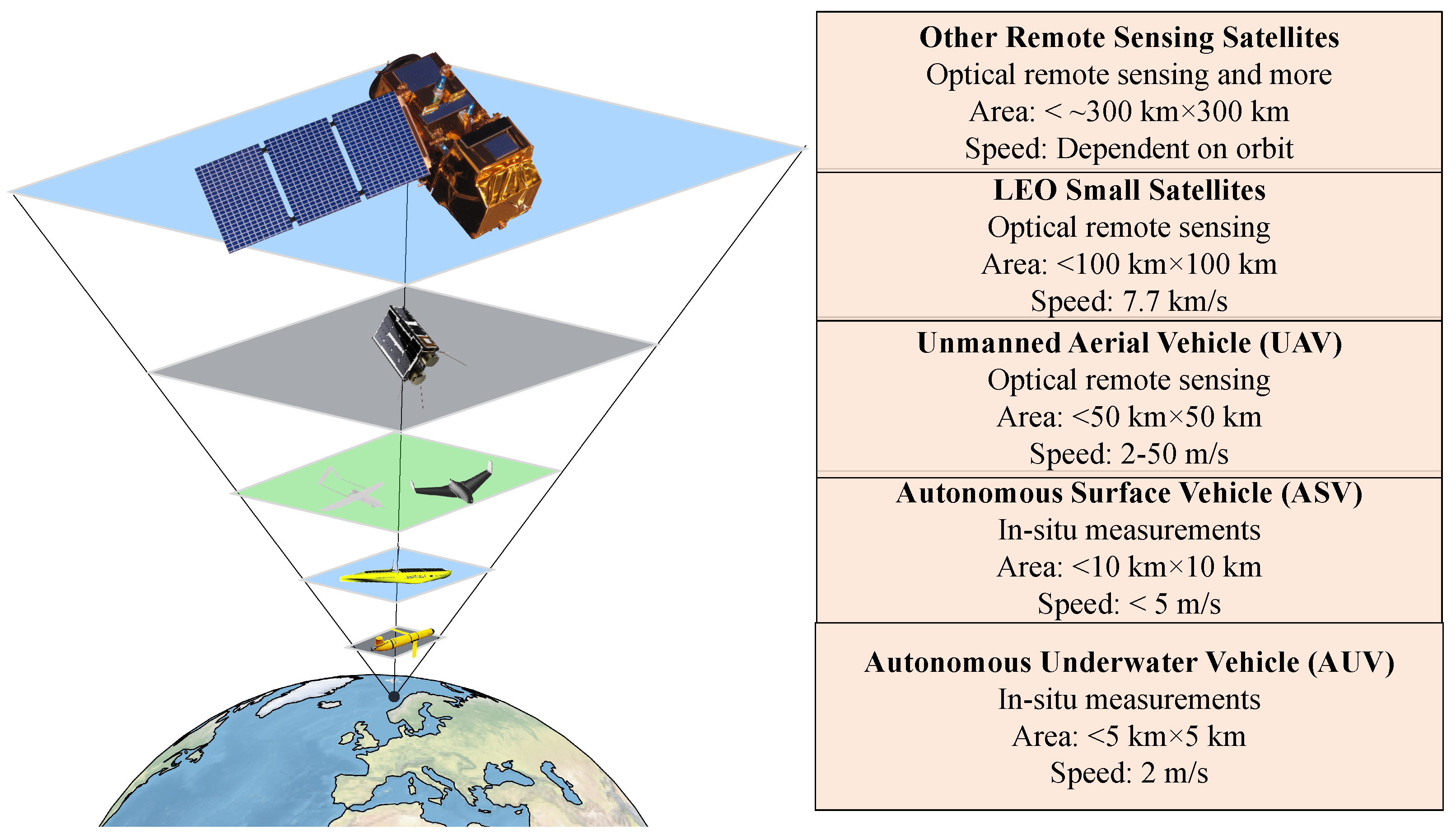
With these scientifically motivated requirements in mind, and the Goal of making oceanographic observations in support of marine research, the HYPerspectral Small satellite for ocean Observation (HYPSO) mission was developed at Norwegian University of Science and Technology (NTNU) [
5]. The HYPSO mission will consist of several small satellites in sun-synchronous Low-Earth Orbit (LEO), starting with the first, the CubeSat HYPSO-1. This satellite program is part of a significant effort towards oceanographic data collection at NTNU Centre for Autonomous Marine Operations and Systems (AMOS), supporting autonomous agents such as Unmanned Aerial Vehicles (UAVs), Autonomous Surface Vehicles (ASVs), Autonomous Underwater Vehicles (AUVs) and buoys in their missions to collect data for ocean-related research. The
observational pyramid, illustrated in
Figure 1, consists of multiple platforms with different capabilities of spectral, temporal and spatial resolution measuring within the same region, as described in greater detail in [
5,
15]. In addition to the autonomous assets developed at NTNU AMOS, these campaign will also rely on the globally available satellite infrastructure intended to continuously cover the entire earth, e.g., the upcoming PACE mission.
The HYPSO satellites are essential elements in the pyramid because they collect data over larger areas with a relatively short revisit time. The revisit time will depend on the given position of the satellite relative to the target and the target’s latitude. The data collected by the satellites will be used to detect features of interest that other autonomous agents can investigate further and in greater detail with optical sensors on UAVs or in-situ measurements [
15]. The pyramid will provide decision support to improve water quality monitoring and to detect oceanographic events such as phytoplankton blooms in the Arctic or even HABs, contributing to the environmental sciences studying marine food chain dynamics. Detection of HABs at an early stage would enable a warning system for both the aquaculture and fishing industries. An HAB warning system requires short revisit times and low latency since HAB dynamics can be fast and complex.
The HYPSO-1 satellite is a 6U CubeSat equipped with a Hyperspectral Imager (HSI) as its payload. The satellite was launched on 13 January 2022 into a 540 km altitude Sun-synchronous orbit, with an orbital period of about 96 min. The payload commissioning phase began at the end of February 2022, and has been ongoing in parallel with the development and advances in the satellite operations scheme, imaging campaigns and gathering data to be used for the calibration and validation of the instrument. The details about the operational schemes used for HYPSO-1 are included as an aid to other universities and institutions seeking to do satellite-based remote sensing. Satellite operations are run by students and researchers in an academic environment, providing both limitations and flexibility to the operations of the satellite [
16]. For instance, exploring new operational scenarios is more attainable at the cost of limited routines and transparent procedures for satellite operations.
Many different satellites and imaging spectrometers have been developed to observe the Earth and ocean color [
1,
2,
4,
6,
7,
8,
17,
18], including several cubesats [
19,
20,
21]. Leveraging the combination of low revisit time, i.e., the period between two possible consecutive observations of a specific target, and fine spectral resolution, is still an active area of research for ocean color remote sensing.
This paper presents images from the first months of operations and describes selected technical specifications such as spatial and spectral resolution and SNR estimated from the in-orbit data. First, in
Section 2, the payload operations’ procedures, and their justifications are described. In particular, it demonstrates that the satellite can capture images within 1.5 h after an area of interest has been identified and that the low revisit time allows for consecutive captures of the same location. Finally, a series of images over Ny-Ålesund, Svalbard demonstrates how a fjord system, an area of interest, can be monitored over an extended time period.
Various parameters to indicate the hyperspectral instrument’s in-orbit performance are given in
Section 3. The spatial resolution is approximated based on scenes with distinct spatial patterns, while the spectral resolution is estimated by comparing radiometrically normalized measurements of the moon with solar irradiance. The overall radiometric accuracy is investigated by comparing HYPSO-1 data collected over RadCalNet sites [
22], and the relative radiometric accuracy between pixels is calculated over a uniform ocean scene. Finally, the SNR per wavelength is modeled and compared to what is achieved by other similar instruments. The results are discussed in light of the original mission objectives, and the way forward is outlined. An overview of mission parameters and resulting payload characteristics related to HYPSO-1 are presented in this, and in earlier publications are summarized in
Table 1.
2. Mission and Payload Operations
The HYPSO mission aims to make agile and near real-time oceanographic observations to support marine research. To achieve this, the ability to capture and downlink data over the desired area with a quick response time, relative to existing satellite systems, has been important when defining the requirements for the mission. From [
5], the following mission Goals are established:
Goal 1: Data latency should be less than
[
25];
Goal 2: Revisit times to dedicated areas of interest should be 3–72 h [
25,
26].
Data latency is the time from when an observation is performed until the final data products are distributed [
5]. However, as the full pipeline to obtain the complete data products has not yet been finalized, the
response time is more relevant to discuss in this paper. In this paper, the
response time is defined as the time from receiving an image request until a capture is planned, uploaded, and performed by the satellite.
The revisit time is the time between successive overpasses with line-of-sight to a target area. In this paper, we elaborate on the effective revisit time, the time between two consecutive imaging operations of the target area by HYPSO-1. The effective revisit time for optical earth observation payloads depends on the time of day, the geographical location, as well as the time of year for targets at latitudes higher than the polar circles. As an example, polar areas can be observed from a sensible angle up to four times a day with 1.5 hr intervals during summer, but during winter, they cannot be observed due to lack of sunlight.
In the following sections, the operational architecture and operations workflow are described and then illustrated with examples showing selected operational capabilities of HYPSO-1.
2.1. Operations Architecture
The mission architecture is divided into a space segment and a ground segment. The ground segment is comprised of the mission operations center and related software tools, with the main Ground Station (GS) located at NTNU in Trondheim. Additionally, the KSAT Svalbard ground station has been used to expand the ground station coverage and to increase downlink capacity at times when the satellite is not in range of the main GS. However, due to the orbit and the geographical proximity of Svalbard and Trondheim, the overall capacity gain of using both locations in succession during nominal operations is small. The orbit of HYPSO-1 gives an average of 10 consecutive communication passes per day over the main GS, from about 07:00 UTC to 22:30 UTC.
At the time of writing, the processing pipeline consists of a CCSDS-123v1 lossless compressing algorithm [
27] typically run on the on-board Field Programmable Gate Array (FPGA). More processing steps will be added to the pipeline later via software updates. After the onboard processing, the data are transferred to the payload controller to await downlinking.
2.2. Operations Workflow
The planning and operational tools have to a large extent been developed during the payload commissioning and operational phases. The HYPSO project has established a digital agile-inspired workflow that allows for continuous incremental development and live tests. During the first weeks of payload commissioning, the imaging schedule scripts were written, uploaded to, and downlinked from the satellite manually. While the tools were developed further and built-in functions from the Mission Control System (MCS) were utilized more, automation of scripts and upload/download tasks became possible.
As with most optical sensors, the HYPSO-1 hyperspectral sensor is hindered by clouds. By requiring a forecast of a cloud-free scene, the number of viable acquisitions over areas of interest becomes very limited. Furthermore, the high revisit time through pointing can to some extent give more capture possibilities over the same area with a shorter revisit time, reducing the impact of clouds. It has been observed that a threshold at around 50% gives satisfactory images, as indicated in
Table 2. This threshold should be changed based on the importance of mapping specific area. In general, a lower cloud coverage is of course desirable.
Since the attitude of the satellite can be controlled, targets can be imaged even if the satellite is not directly above them. The elevation angle between the satellite and the target area of interest also affects the imaging quality with regard to parameter retrieval. At lower elevation angles, i.e., more off-nadir, the observations are more skewed and have a poorer spatial resolution. Additionally, adverse effects from the atmosphere are also observed. This is exhibited by blue color being more prominent in the image possibly due to Rayleigh scattering [
28]. A lower limit of elevation angle is suggested in
Table 2.
The range of exposure times for HYPSO-1 is given in
Table 2. The optimal values depend on the imaging scene and the solar zenith angle. The response of the imaging sensors used varies linearly with the incident light, but easily becomes saturated over clouds and deserts. As a result of this linear response, there is a trade-off between acquiring as much light over dark objects, e.g., ocean targets, and being over-exposed over brighter targets.
The frame rate sets an upper bound for the exposure time. With a higher frame, the spatial resolution can also be improved, but this comes at the cost of lower exposure time. Conversely, lower exposure time can reduce SNR as less light is collected. The highest reliable frame rate for the nominal cube size can be found in
Table 2.
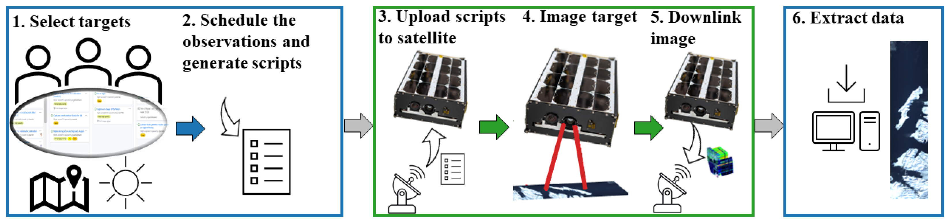
Satellite and imaging operations for the HYPSO-1 mission are primarily planned on a weekly basis, with smaller updates three times a week to account for weather forecasts or other events. The general workflow for the pass planning is shown from left to right, following the arrows in
Figure 2. During a planning session, a prioritized list of potential targets is selected. Targets are selected based on the timing, ongoing geophysical or biological phenomena, field campaigns, weather forecast, and whether they can be observed by other agents. After all this is considered, the final observation schedule is planned and a script is generated for the next few days. The scripts are tasked for upload and execution on the satellite in the MCS, which schedules upload of the scripts to the satellite during a subsequent ground station pass. At the start time defined by the scripts, pointing is activated, the payload is powered on and an image is captured. The capture time is on the order of one minute. It should be noted that the capture time can be altered, but the data throughput is predominantly limited by the ≈1 mbit/s bandwidth of the S-band radio communication. The collected data are merged with the corresponding metadata before being transferred to the Payload Controller (PC), a designated subsystem for data storage and subsequent radio transmission onboard the satellite. The image data are automatically downlinked at the next ground station pass by the MCS. Downlink of a single capture may require more than one ground station pass, as an example in
Table 3 shows. After being downlinked, the data are extracted from the MCS database and processed.
New observations can be added to the schedule on short notice. Examples of situations that make altering the schedule necessary include a sudden change in solar activity (powering off non-essential subsystems on the satellite to avoid damage caused by radiation from a solar flare), news about algal blooms, and requests made by researchers or scientists.
During the first months of operations, 5–6 captures per day were typically planned for nominal operations because they fit within the downlink capacity limit for compressed raw data. More captures can be performed per day for a short period, but a backlog for downlink accumulates. The backlog must be downlinked at a later stage, which limits the downlinking time which can be dedicated to new captures. Assuming undisturbed operations, around 450 MB can be downlinked per day [
29], equivalent to 5–6 captures when using a single ground station (Longyearbyen, Svalbard or NTNU Trondheim).
Imaging targets geographically close to the ground station reduce the time that can be dedicated to downlinking data because the ground station communication then overlaps with an observation. Effective downlinking of data requires pointing the satellite antenna toward the ground station, which is not possible while pointing the camera to the targeted area, as the antenna and camera is fixed to the spacecraft. Only the ground stations in Norway and at Svalbard are currently in use, causing the largest downlink capacity reduction for imaging operations over the Arctic, Norwegian areas and other parts of northern Europe. To mitigate this, more ground stations that support S-band radio communication spread out at other locations on the earth could be included in the ground segment.
2.3. Time Schedule of a Quick-Response Capture
As stated in mission Goal 1, the data latency should be under 1 h. This is important when supporting field campaigns, autonomous agents in the field, or providing data on oceanographic events such as algal blooms or HABs, during which a quick response is needed.
An example of setting up a quick-response plan, covering the tasks of choosing targets, scheduling and generating scripts, uploading scripts and acquiring data from the satellite (steps 1 to 4 of the operational workflow), is shown in
Table 3. The image capture process, from image capture planning until the image capture, takes less than 1.5 h. The downlinking time for the raw data, however, depends on ground station availability, and the size of the observation. This causes the full planning, capture, and downlink process to be performed in about 5–6 h. When the onboard processing pipeline can produce operational data of a much smaller size, the desired time constraint can be met. For targets near the equator, there is normally only a single possible capture pass per day when taking the elevation requirement into account, while targets with higher latitudes (north or south) can be imaged multiple times per day during polar summer.
2.4. Short Revisit Time at High Latitudes
Mission Goal 2 states that the revisit time of dedicated areas of interest should be 3–72 h, to monitor the temporal changes on an hourly time-scale of ocean color.
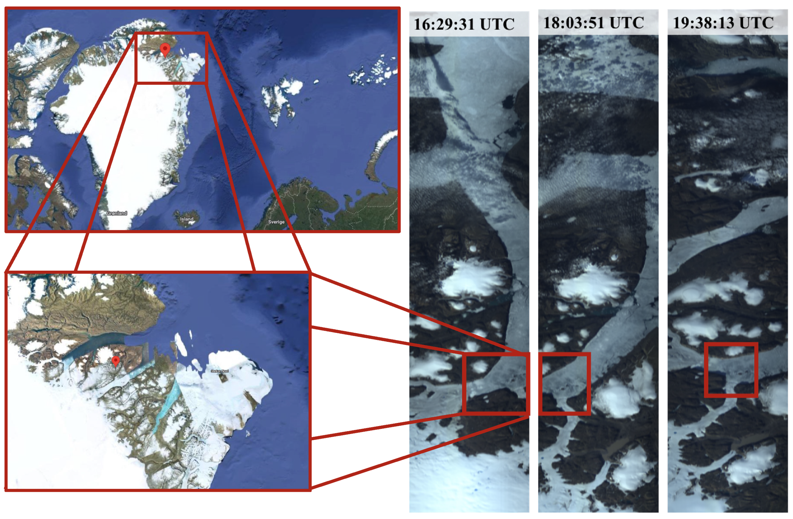
One example of low revisit times is a series of three consecutive captures taken over the same location in Greenland (81.7°N, 27.3°W). RGB composites are shown in
Figure 3. A common region in each of the pictures is shown with red rectangles. The different imaging angles for each pass complicate co-registration. The low revisit time can be valuable and utilized when the satellite is part of targeted research campaigns, as described in the next section.
2.5. Research Campaigns
During the spring of 2022, the HYPSO-1 satellite supported several research campaigns. Among these were a joint mission in Frohavet (outside the Trondheim fjord in Norway) in April 2022, described in [
30], a research campaign in Kongsfjorden in Svalbard, Norway, in May 2022 (with additional data collected during the summer of 2022) and surveillance of Mjøsa, the largest lake in Norway, looking for an indication of HABs that may harm the water quality. In the following, some of the data from the research campaign in Kongsfjorden are presented and discussed.
Kongsfjorden is a glacial fjord located on the west of the Spitsbergen coast in Svalbard, at the coordinates 78°59′N, 11–12°E, surrounded by mountains, calving glaciers, rivers and the small town of Ny-Ålesund [
31]. Normally, a spring bloom initiates biological production in April–May. Therefore, a joint research campaign was conducted in the period from 19 through the 29 of May 2022 by NTNU AMOS, University of Tromsø—The Arctic University of Norway (UiT) and the University Centre in Svalbard (UNIS). The research campaign focused on the detection and mapping of biological and environmental variables in the fjord using multiple sensor platforms such as UAVs, ASVs, AUVs, Remotely Operated Vehicles (ROVs), water samples collected from boats and in situ samples collected by divers, as envisioned with the observational pyramid. The details and outcomes of the campaign are not presented here.
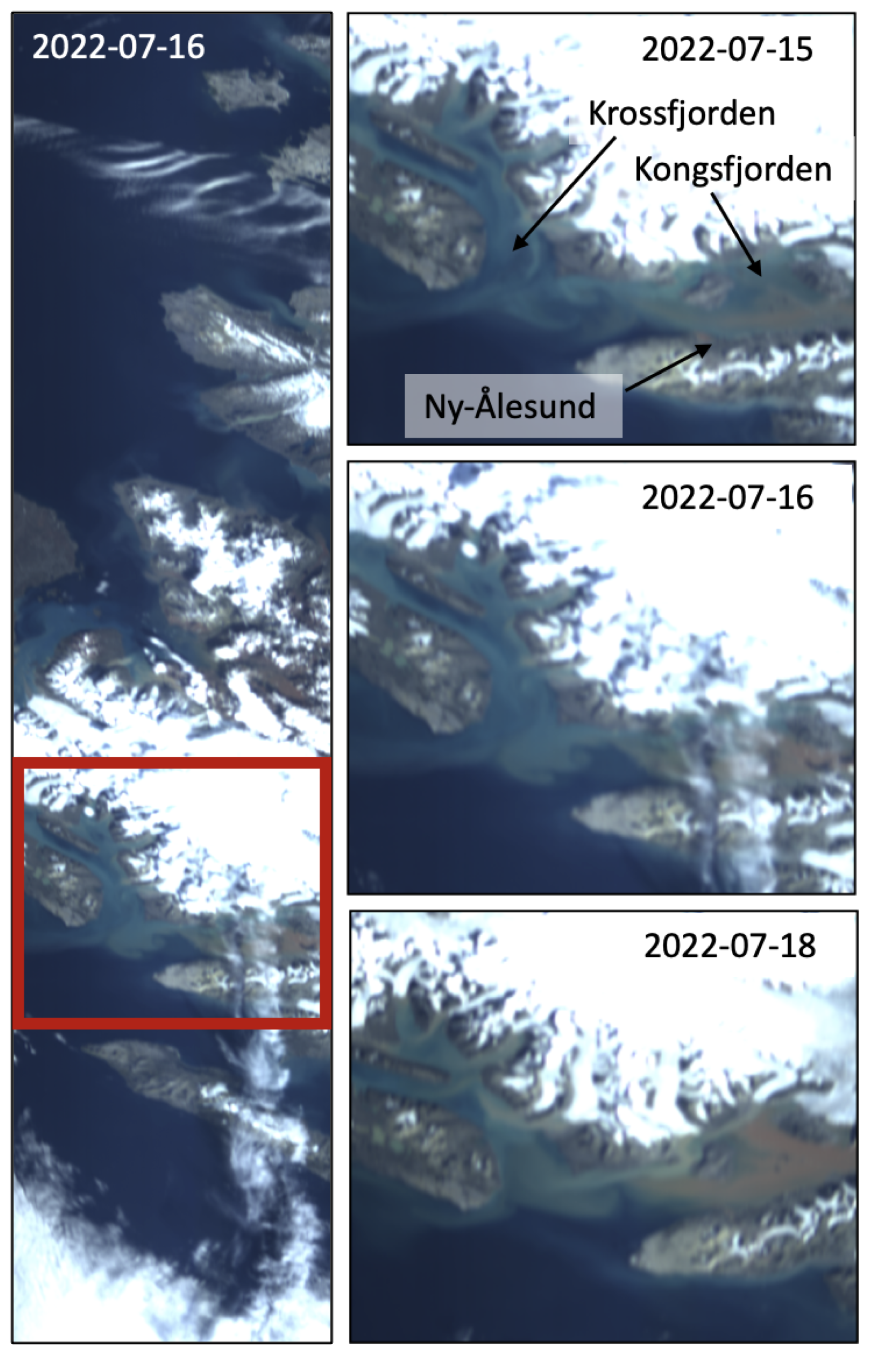
HYPSO-1 supported this research campaign by collecting hyperspectral data 2–4 times a day over Kongsfjorden during the main campaign period, and by continuing to monitor the area over the summer. In total, more than 30 images were acquired, excluding those deemed useless due to extensive cloud cover.
An example of three of the images captured over Kongsfjorden by HYPSO-1 during the summer is shown in
Figure 4. Daily changes in surface features in the fjord confirm the need to map such areas repeatedly to capture these dynamic events. The water color changes from a mix of green and light brown to deep reddish brown over only a couple of days. This suggests the presence of run-off from rivers and/or glaciers containing minerals with oxidized iron. Different colors indicate distinct minerals originating from various surrounding rivers, which might make it possible to trace them back to the river source [
32]. In addition, the movement of turquoise patterns between Kongsfjorden and Krossfjorden can indicate Total Suspended Matter (TSM) from glacial run-off. There should be little CDOM present in the waters around Svalbard as there is no topsoil and not many plants. However, some chlorophyll-a present in the water might contribute to a more greenish color as blue and red light would be absorbed. The hyperspectral data from HYPSO-1 can help establish the content of the water by investigating the spectral signatures.
3. In-Orbit Payload Performance
The HSI onboard HYPSO-1 is a push-broom hyperspectral imager with a transmissive grating design, assembled using Commercial-Off-The-Shelf (COTS) components, as described in [
23]. The main design specifications are a spectral range of 400 to 800 nm, theoretical spectral resolution of 3.33 nm at 600 nm, spatial resolution of 100 m × 100 m (defined from the HYPSO-1 orbit) and a Top-of-Atmosphere (ToA) SNR of 100 [
5,
23]. From pre-launch calibration, the full spectral range imaged on the sensor is 226 to 961 nm, but only the 400 to 800 nm range is used for nominal operations due to a low signal below 400 nm and second-order diffraction effects appearing above 800 nm. The spectral resolution was found to be less than 4.5 nm for all wavelengths, and the spatial focus was shown to be best around 600 nm, which is approximately in the center of the image [
24].
The instrument was designed and built for the HYPSO mission, based on the following Goals from [
5]:
Goal 3: Images should have spatial resolution better than 30–100 m per pixel [
3,
11];
Goal 4: The raw hyperspectral data should have a spectral resolution of about 5 nm, or better, for VIS-NIR wavelengths [
3,
11];
Goal 5: The SNR at ToA should be greater than 400 in visual wavelengths for open ocean water [
33], and atmospherically corrected SNR of water-leaving signals should be between 40–100 [
34].
The spatial resolution Goal may be achieved either before or after applying corrections and image capture in a slewing maneuver combined with imaging enhancing techniques such as super-resolution [
5]. This has not yet been fully explored for the HYPSO-1 data, and the spatial resolution is estimated based on the raw data. Imaging with the slewing maneuver [
5] leads to a larger number of scan-lines over a smaller area. With image processing, this extra information over a given area is expected to improve the spatial resolution. For Goal 4, the spectral resolution should be 5 nm preferably for all data collected. For HYPSO-1 nominal data, a spectral binning factor of 9 is used, aligning the spectral sampling with the theoretical spectral Full-Width at Half-Maximum (FWHM). This will affect the estimated spectral resolution. Both binned and non-binned data will be investigated here. For Goal 5, related to the noise characteristics of the data, the ToA SNR is estimated using a nominal image cube with binned data from HYPSO-1. The binned cube is compared to data from other sensors.
3.1. Spatial Resolution
The spatial resolution of an imaging system describes the size of the smallest discernible feature within an image. It is an important performance indicator that helps users determine if the imagery is suitable for a particular analysis [
35,
36,
37].
Two important metrics used when assessing spatial resolution are Ground Resolvable Distance (GRD) and Ground Sampling Distance (GSD). The GRD is the smallest distance between two spatially distinct point features such that they can be distinguished in the image. The GRD can be measured or computed in several ways [
36]. The GSD is the ground projected distance from one spatial pixel to the next in the image, the pixel-to-pixel distance. Due to imperfect optics, the GRD may be larger than the GSD [
36]. Thus, a smaller GSD in value does not guarantee that smaller features are resolvable. The GRD, however, considers all effects influencing the spatial resolution. The theoretical GSD for HYPSO-1 is discussed in more detail in [
5].
In this section, we estimate the spatial resolution in units of pixels by estimating the FWHM of the Line Spread Function (LSF). The estimated FWHM is used to quantify the GRD. In addition, using direct geo-referencing, the GRD is computed from the pixel level spatial resolution and compared to the simulated GSD from [
5].
3.1.1. Ground Resolvable Distance (GRD)
Here, first a qualitative and then a quantitative characterization of the pixel-level spatial resolution for HYPSO-1 in terms of GRD is presented. The aforementioned work does not discuss the potential adverse effects the atmosphere can have on resolving ground targets, and it is not further discussed here.
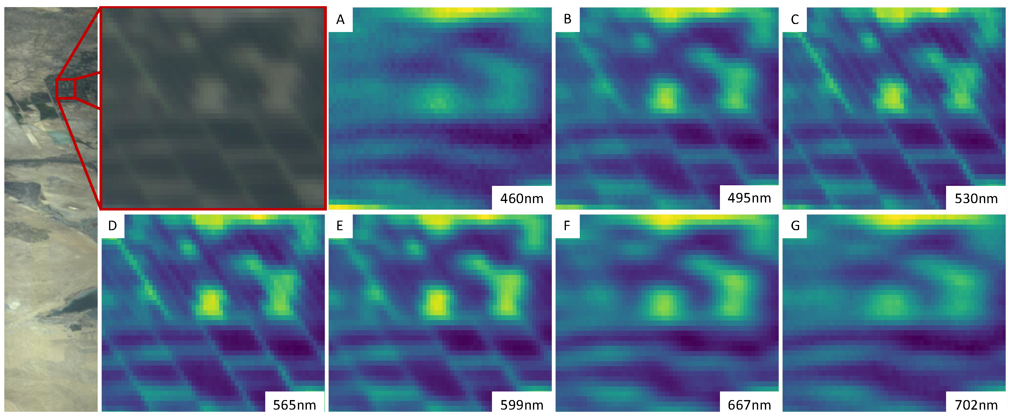
In
Figure 5, an image from an agricultural field near the Euphrates/Tigris estuary is used to assess HYPSO-1’s sharpness. The lines in the field are due to roads and irrigation lines. The width of the lines running diagonally in the image is found using high-resolution satellite imagery to be about 50 m across. Selected bands across the spectral range are shown of the field closeup. The sharpness increases from 400 nm to about 530 nm and then decreases again from 565 nm to 800 nm. The sharpest bands are around 530 nm to 565 nm. Below 460 nm, and above 702 nm, the spatial images appear blurry. Worse spatial resolution at above 600 nm and below 500 nm is also consistent with the results from
Figure 6, described in the following paragraphs. Note that the increased blurriness is predominantly in the horizontal direction of the images, which corresponds to the across track direction. The blurriness in the vertical or along track direction is in large part determined by the way the push broom scanning is performed as opposed to optics.
The quantitative sharpness analysis used the spatial resolution assessment method described in [
37,
38]. This is a processing pipeline for sharpness assessment for remote sensing data originally developed for sensors with a poorer spectral resolution. The method estimates multiple spatial resolution metrics, among them the FWHM of the LSF and the Relative Edge Response (RER). This estimation is carried out for several automatically detected suitable edges and repeated for every band.
To estimate the LSF FWHM, an image of a thin (meaning smaller than the GSD) line with sufficiently distinct reflectance properties compared to the scene background is to be imaged. Alternatively, LSF can be estimated by differentiating the edge response, or the Edge Spread Function (ESF). The ESF is found by considering the sharp edge between two contrasting regions in the image [
35]. Values for the LSF FWHM between 1.0 and 2.0 are associated with a balanced sharpness performance, while values higher than 2.0 are associated with blurry images. Ideally, one would have a LSF FWHM average close to 1.5 [
37]. For comparison, the HICO instrument reported a maximum FWHM of the Point Spread Function (PSF) 1.6 [
8].
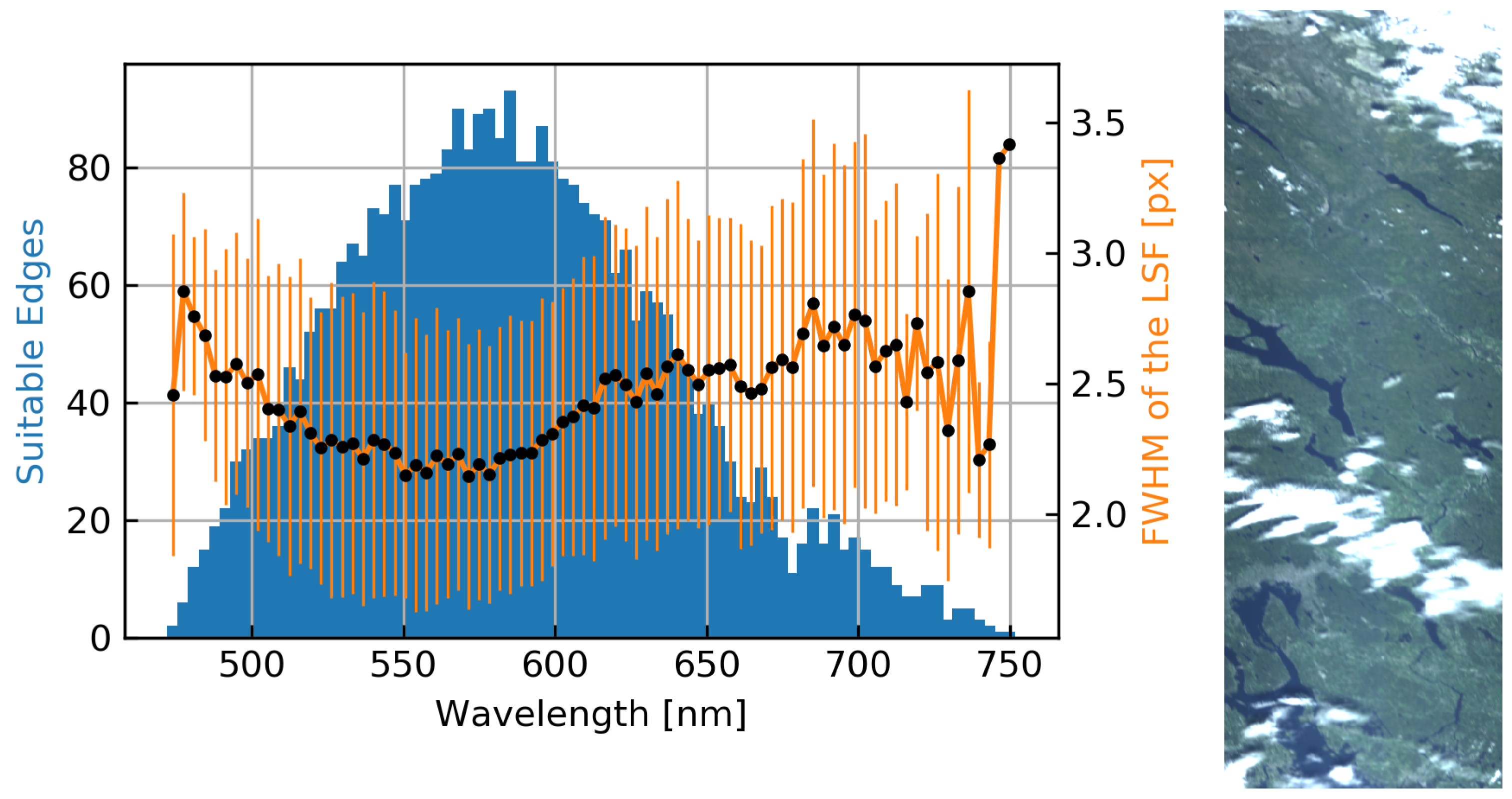
Multiple images of various scenes were analyzed, with similar results. Results from the particular image in
Figure 6 are shown as most edges were found in this image which is an indication of confidence in the results.
Figure 6 shows the results of the FWHM of the LSF estimation, with the image on which the assessment was performed to the right. The plot to the left in
Figure 6 shows the mean of the estimated LSF FWHM for each band in a data cube, in addition to a histogram of the number of suitable edges used for the sharpness assessment for each band. Some bands at the extremities are removed as no suitable edges were found. The edges found by the sharpness assessment are almost exclusively in the across-track direction. Thus, this analysis characterizes only the across-track resolution. The mean LSF FWHM across all bands is 2.45 pixels. The best-performing bands have a LSF FWHM average below 2.4 pixels in the range 510 nm to 600 nm. The LSF FWHM for the sharpest band at 565 nm is 2.192 pixels. The standard deviations are higher than the 0.2–0.4 pixels typically found in satellite imagery. The resolution in worse-performing bands is beyond three pixels in terms of LSF FWHM.
Super-resolution methods and panchromatic sharpening that leverage the sharpest wavelengths could be used to improve the resolution of the higher and lower wavelength bands. Investigation of potential venues for image enhancements is a topic for future research [
39].
3.1.2. Ground Sampling Distance (GSD)
Due to the ability to point off-nadir to increase revisit time, geometric distortions, similar to the bowtie effect due to the constant angular resolution of the instrument, cause the GSD to increase with a larger off-nadir angle, and with it also the ground projected GRD in terms of meters [
40]. The GRD degrades with an increase in off-nadir angle.We use Attitude Determination and Control System (ADCS) telemetry, a camera model, and other parameters to directly geo-reference the pixels of an image, from which the off-nadir angle varying GSD is determined on a per-image basis. Forming the product between the GSD in terms of meters and the LSF FWHM of the optics in terms of pixels, an image-specific GRD is determined.
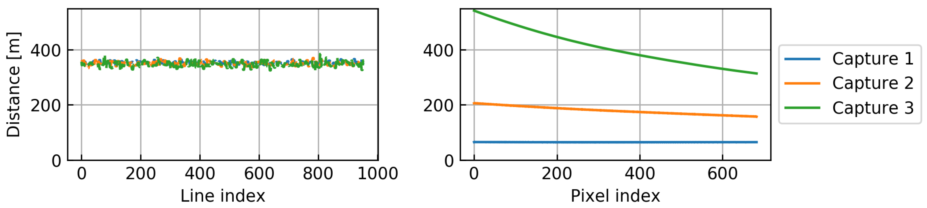
Figure 7 shows the GSD determined using direct georeferencing of three captures with different off-nadir angles.
Table 4 shows more information about the three captures, in particular average GSD, in addition to the estimated GRD. The left plot in
Figure 7 shows the along track GSD of the center pixels within each line of the data cubes (pixel index 341). The apparent noise is due to a time-stamping inaccuracy. The right plot shows the GSD across track of the middle line (line index 477) in the data cubes. The across track GSD increases as expected with a larger off-nadir angle. The along-track GSD is unchanged due to no dependence on off-nadir angle. The GSD close to the nadir is about 60–70 m, while it reaches ca. 500 m, 400 m on average across in the most off-nadir case. Approximately 63° is the highest off-nadir angle HYPSO-1 acquire hyperspectral scenes without viewing past Earth’s horizon.
3.2. Spectral Resolution
Spectral resolution of an HSI is typically measured in the laboratory prior to launch, as carried out for HYPSO-1 in [
24]. A method to estimate spectral resolution in orbit is to compare the recorded spectrum with a reference spectrum [
41]. The high-resolution reference spectrum is convolved with a simulated instrument response at different spectral resolutions to produce a simulated spectrum for each spectral resolution. These spectra are further compared to the recorded spectrum by HYPSO-1, and the most similar one gives an indication of which spectral resolution HYPSO-1 achieves.
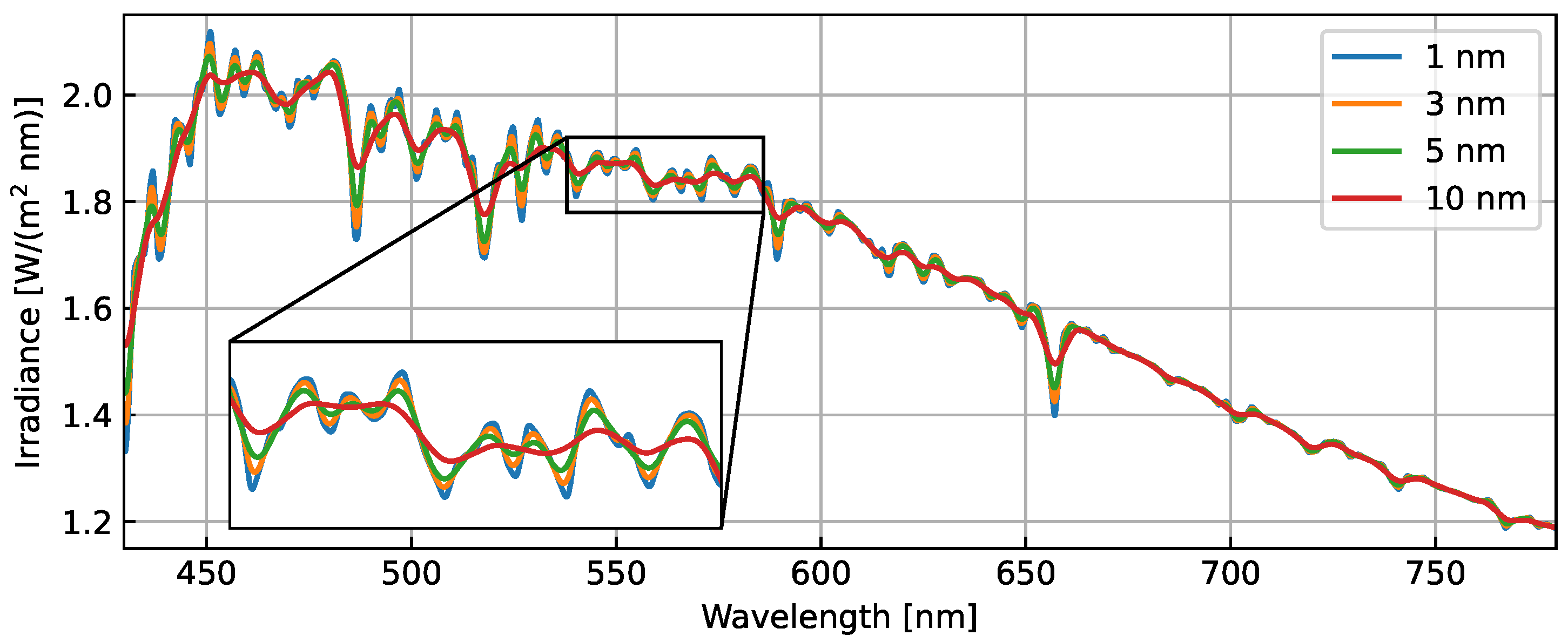
Here, the Solar spectrum (1985 Wehrli Standard Extraterrestrial Solar Irradiance Spectrum) with known Fraunhofer lines is used as the reference spectrum, while the recorded spectrum is reflected light off the Moon. The spectral range from 430 nm to 780 nm is investigated due to low amounts of recorded signal below 430 nm, and to avoid second order effects appearing above 780 nm.
The instrument response is simulated as a perfect instrument response, represented by a triangular function of different half-widths to represent different spectral resolutions. The solar spectrum convolved with a set of instrument responses is shown in
Figure 8. For wider triangular functions, the peaks that are close together get merged. This is observed in the 10 nm resolution response (red line).
HYPSO-1 can capture data with and without binning. For nominal operations, only a subset of the available pixels stored, namely the center 1080 pixels in the spectral range and the center 684 pixels in the spatial range of the spectrogram. During nominal operations, binning of nine spectral pixels by summation is applied. Binning data reduce noise and data size. However, binning spectral pixels can also affect the spectral resolution. The spectral resolution is therefore estimated for both full resolution data, and data where binning is applied. Another method to reduce noise when imaging uniform areas is to average the signal from consecutive frames. Ten frames are therefore averaged and compared to the original and binned data in
Figure 9. Only the center of the slit image is used to avoid smile effects. It can be seen that one full resolution frame has more noise fluctuations than both the 10 frames average and the binned data, and that the binned data are slightly worse at resolving the curves in the spectrum due to less datapoints.
For further analysis, a low-pass filter is applied to smooth the full resolution data to reduce noise, and a high-pass filter applied to both the HYPSO-1 data and the reference data to remove slow intensity changes. The datasets are then normalized by scaling with their maximum values. The resulting filtered and normalized responses of the reference spectrum and full resolution data (1 frame) are shown in
Figure 10, showing comparable features from the Fraunhofer lines in the datasets.
The solar spectrum was simulated at resolutions between 3.3 nm (theoretical limit of HYPSO-1) and 10 nm, with 0.1 nm steps. The spectra were compared by using Root Mean Square Error (RMSE) between the HYPSO-1 spectrum and reference spectra, and best fit determined as the one with the lowest RMSE value. The results are presented in
Table 5. The solar spectrum with spectral resolution of 5.4 nm was found to be the best fit within the range of 430 nm to 780 nm for the full resolution data (1 frame) and 5.6 nm when 10 frames were averaged first. With binning, the same analysis gives the average spectral resolution over the same range to be 8.2 nm.
It was shown in [
24] that the spectral resolution varies with wavelength, where it was measured to be between 3.5 and 4.5 nm for HYPSO-1 prior to launch (for full spectral resolution data). The best resolution was found above 700 nm, while wavelengths between 430 nm and 700 nm had resolution calculated to be roughly between 4 nm and 4.5 nm. The analysis here was therefore repeated for only parts of the spectra, in 50 nm bands starting at 430 nm and ending at 780 nm, i.e., 430–480, 480–530, etc. The best fit spectral resolutions in those bands and RMSE of the fit are presented in
Table 5. The highest (lowest number) estimated spectral resolution of the full resolution data (both 1 frame and 10 frames average) is 3.4 nm, found in bands 630–680 and 730–780, which is close to the theoretical limit of 3.3 nm 3.3 nm. The lowest (highest number) for the full resolution data are 6.6 nm (1 frame) and 7.2 nm (10 frames average), which is found between 530 nm and 580 nm. This coincides with the trends seen in [
24]. For the binned data, the highest spectral resolution is found at 730 to 780 nm, and is 4.0 nm, while the lowest is found at 430 nm to 480 nm to be 9.60 nm. Similar to the findings in [
24], the resolution is best at longer wavelengths (above 600 nm), and worse for the binned data. The signal recorded for short and long wavelengths is relatively low so SNR is lower, as seen in
Figure 9. In the range 730–780 nm, the estimated spectral resolution is worse for the full resolution single frame than the binned data. This is likely to be because the binned data are smoothed so the noise is reduced.
The RMSE value gives insight into how large deviation was found between the solar spectrum of estimated resolution and the measured HYPSO-1 spectra, with low RMSE values meaning similar spectra. However, mismatch between the spectra can also come from different intensities not being fully filtered out, leaving residue from the reflected light of the scene (the Moon), or from spectral shifts between the spectra. It is therefore important to make sure the spectra are properly filtered and aligned before the analysis. One reason for the RMSE varying between the different spectral ranges can be due to different features at different locations in the spectrum, making some regions easier to match up than others. It can be noted that the 630 to 680 nm range has high RMSE compared to the other ranges, most likely due to few features being present in this region. The RMSE values are also generally higher for the single full resolution frame than for the 10 frames average, indicating that averaging frames reduces noise and makes features in the spectrum more visible.
The estimated spectral resolution is overall slightly worse than what was found during pre-launch calibration. This can be due to the pre-launch measurements using spectral lamps, looking at few spectral lines at the time and estimating the spectral resolution by calculating the FWHM. The method used here, comparing the full recorded spectrum with simulated solar spectra of different resolutions, gives an indication of what spectral resolution can be achieved, but might not be as accurate as using spectral lamps and calculating the FWHM. The results presented here shows that a spectral resolution of about 5 nm is a realistic performance of the instrument in some spectral ranges, but further investigations should be carried out to estimate the exact spectral resolution as a function of wavelength with the in-orbit data.
3.3. Top-of-Atmosphere Radiometric Validation
Radcalnet provides top-of-atmosphere reflectance data with uncertainties at a 10 nm resolution in the range of 400–1000 nm at intervals of 30 min. The data from RadCalNet are intended to be representative for a nadir-viewing perspective [
42]. Data collected near RadCalNet sites are used in this section to evaluate the radiometric accuracy of HYPSO-1. The top of ToA reflectance is a measure of the amount of light that is reflected off the Earth and its atmosphere when illuminated by the sun. It is calculated using the following formulas [
43]:
where
is the ToA reflectance,
is the radiance,
is the distance between the Earth and the sun,
is the mean solar exo-atmospheric irradiance, and
is the Solar zenith angle. This formula is used to compare the ToA reflectance of data from the HYPSO-1 instrument with data from selected RadCalNet sites [
42,
44]. These sites provide inferred ToA reflectance. As a result, it is possible to compare the measurements from HYPSO-1 using the calibration coefficients acquired on ground with the data provided by RadCalNet without further processing.
Each line in a HYPSO-1 capture has its solar zenith angle, and each band has its mean solar exo-atmospheric irradiance. The analysis of the radiometric sensitivity of HYPSO-1 considers the ToA reflectance. This section gives a comparison between the ToA reflectance from HYPSO-1 with selected RadCalNet [
42,
44] sites. The instrumented RadCalNet sites provide inferred ToA Reflectance. No compensation of atmospheric effects is needed by comparing the HYPSO-1 data with the inferred ToA reflectance.
To calibrate the measured radiometric intensity of the HSI payload, the ToA reflectance values measured by HYPSO-1 are compared to Sentinel-2 data [
45] and RadCalNet test sites [
22,
44], which have hyperspectral cameras that measure the bottom-of-atmosphere reflectance and, in turn, compute the ToA reflectance. The meta information from the different data sources are given in
Table 6 and
Table 7.
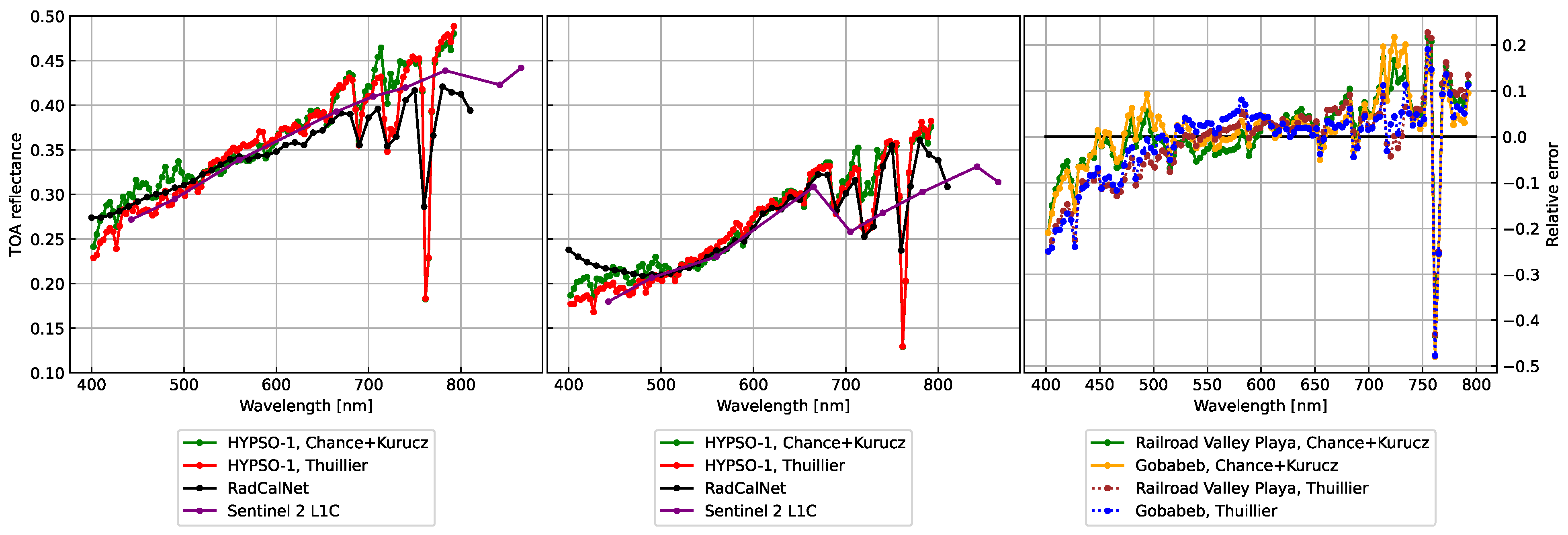
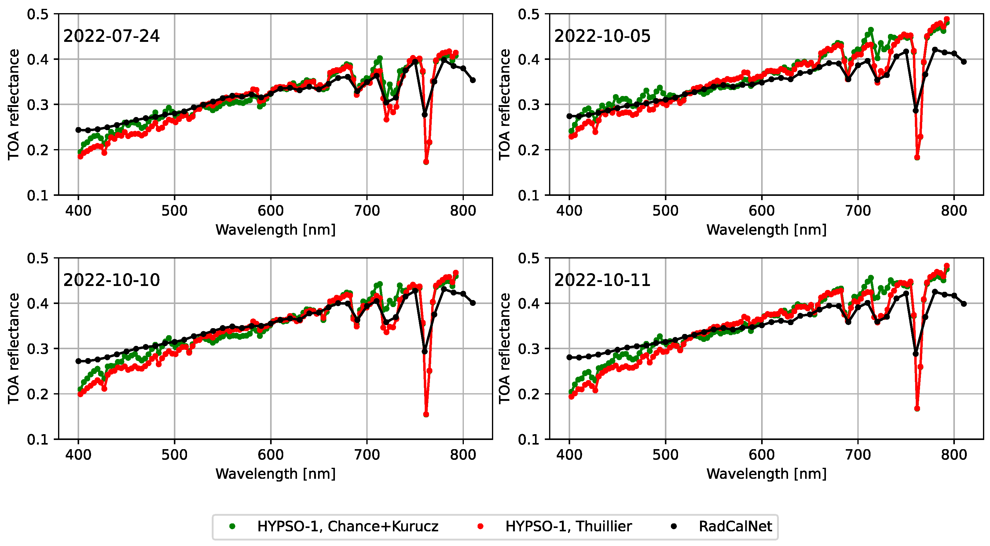
Figure 11 show the estimated HYPSO-1 ToA reflectance compared to the RadCalNet ToA reflectance and Sentinel-2 ToA reflectance.
Figure 12 shows the estimated HYPSO-1 ToA reflectance compared to the RadCalNet ToA reflectance from the Railroad Valley playa test site. The calculation of ToA reflectance in
Figure 11 and
Figure 12 was performed using two different solar spectra. The first solar spectrum is the ChKur solar spectrum [
46], which is also used for the Landsat missions [
43]. The second solar spectrum used is the Thuillier solar spectrum [
22,
47]. Both solar spectra were used to calculate the TOA reflectance in
Figure 11 and
Figure 12, and the latter has a higher spectral resolution. HYPSO-1, at wavelengths beyond 650 nm, frequently reads higher ToA reflectance than RadCalNet, causing a relative error for wavelengths above 700 nm to occasionally reach 20%. When using the Thuillier solar spectrum, which has a finer spectral resolution, the relative error between 700 nm and 750 nm is lower than when using the ChKur solar spectrum. In this region, there are oxygen bands that will be heavily affected by the spectral resolution of the measured signal. At wavelengths between 761 nm and 765 nm, the ToA reflectance HYPSO-1 reads are lower than RadCalNet. This can be explained by the 760 nm oxygen absorption line being better resolved by HYPSO-1 than RadCalNet. In [
22], the DLR Earth Sensing Imaging Spectrometer (DESIS), which is a hyperspectral imaging spectrometer, Level 1 product (ToA reflectance) are compared with RadCalNet ToA reflectance. They state that the DESIS spectra are inconsistent at wavelengths lower than 430 nm due to atmospheric scattering. An inconsistency is also observed when comparing the HYPSO-1 ToA reflectance with RadCalNet ToA reflectance at these wavelengths.
Figure 11 provides a comparison of the ToA reflectance at the RadCalNet test site in Gobabeb with HYPSO-1 ToA reflectance and Sentinel-2 ToA reflectance. The analysis given here used images that were captured one day apart from the RadCalNet data since there were no captures from the same day during the campaign period. The ToA reflectance changes every day and throughout the day. The RadCalNet sites are located to be pseudo-invariant, meaning that their reflectance properties are stable relative to other natural targets [
42]. It is an important factor when analyzing the ToA reflectance and the relative error for the Gobabeb captures in
Figure 11.
3.4. Spatial Destriping
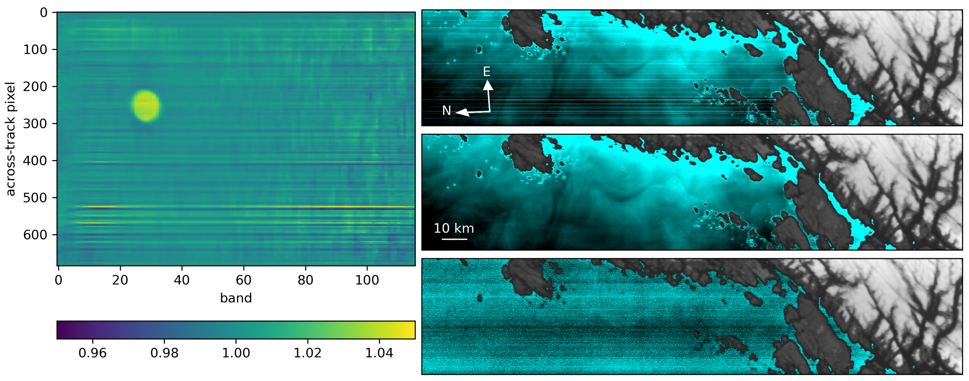
Stripes in hyperspectral datasets commonly limit their use [
48]. One of the major causes of striping in push–broom scanning is differences in the radiometric sensitivity between pixels. Even sensitivity differences of a few percent between pixels can lead to stripes in the collected data. The differences can be systematically mitigated by improving the estimate of the relative radiometric sensitivity.
The relative sensitivity differences between the pixels of the HYPSO-1 sensor are estimated over a mostly uniform ocean scene. Clouds and land are excluded from the analysis, and the laboratory radiometric calibration is applied to the data. Because the expected correction is multiplicative, the scene is analyzed after a logarithm is applied.
As the scene is uniform, most of the across-track variation is due to stripes. The magnitude of the stripes within each band is determined by computing the difference of each along-track column of pixels from its across-track neighbor, pixel by pixel. The median of the differences is taken to be the magnitude of each stripe, in order to limit the effect of spectral features which may be present in the ocean. The cumulative sensitivity differences are then computed relative to mean intensity, and the mean is removed for each wavelength. The multiplicative correction to the relative sensitivity differences is then the exponential of the cumulative differences (
Figure 13). The correction is filtered to remove vertical stripes which originate from the smile artifact [
24]. The dust particle moved during launch, as seen in
Figure 13, and new calibration coefficients were needed to compensate for this movement.
The effect of the multiplicative radiometric correction is evaluated on a second ocean scene. The spectral pixelwise variance between the original and corrected test scene is about 9.1% of the total variance of the former. Principal Component Analysis (PCA) is applied to ocean pixels of the scene, and the different components are inspected for stripes to evaluate the correction. Before the multiplicative correction, stripes are visible starting at the first component, but after the multiplicative correction, they are not visible until after the sixth component. The remaining variance in these higher components is about 3.3% of the total variance, of which stripes are only one part. Therefore, about 11% of the variance was due to stripes prior to the correction and so the multiplicative correction reduces striping by almost a factor of four in this sense. This result will be scene dependent but gives an indication of the effect from the correction.
The correction can be applied to all HYPSO-1 images because it is multiplicative rather than additive. It is combined with the standard radiometric calibration for conversion from digital number to ToA radiance. The change in radiometric sensitivity between laboratory calibration and the observing of the test image is likely due to the relocation of dust and small particles within the imaging system arising from vibration during the spacecraft lau, as discussed further in [
49]. The scene used to characterize and correct for the striping effect is of the open ocean, a relatively dark target with limited signal to measure. Utilizing clouds may produce better outcomes; however, due to the linear response of the imaging sensor, images easily become oversaturated over bright targets. Although utilizing a uniform ocean scene for spatial destriping is effective for the spectral range of 430 nm to 600 nm, striping effects still appear above 600 nm. The calibration coefficients for each capture should improve with time. A more campaign to achieve a flat radiometric response is planned for the future.
3.5. Spectral Signal-to-Noise Ratio
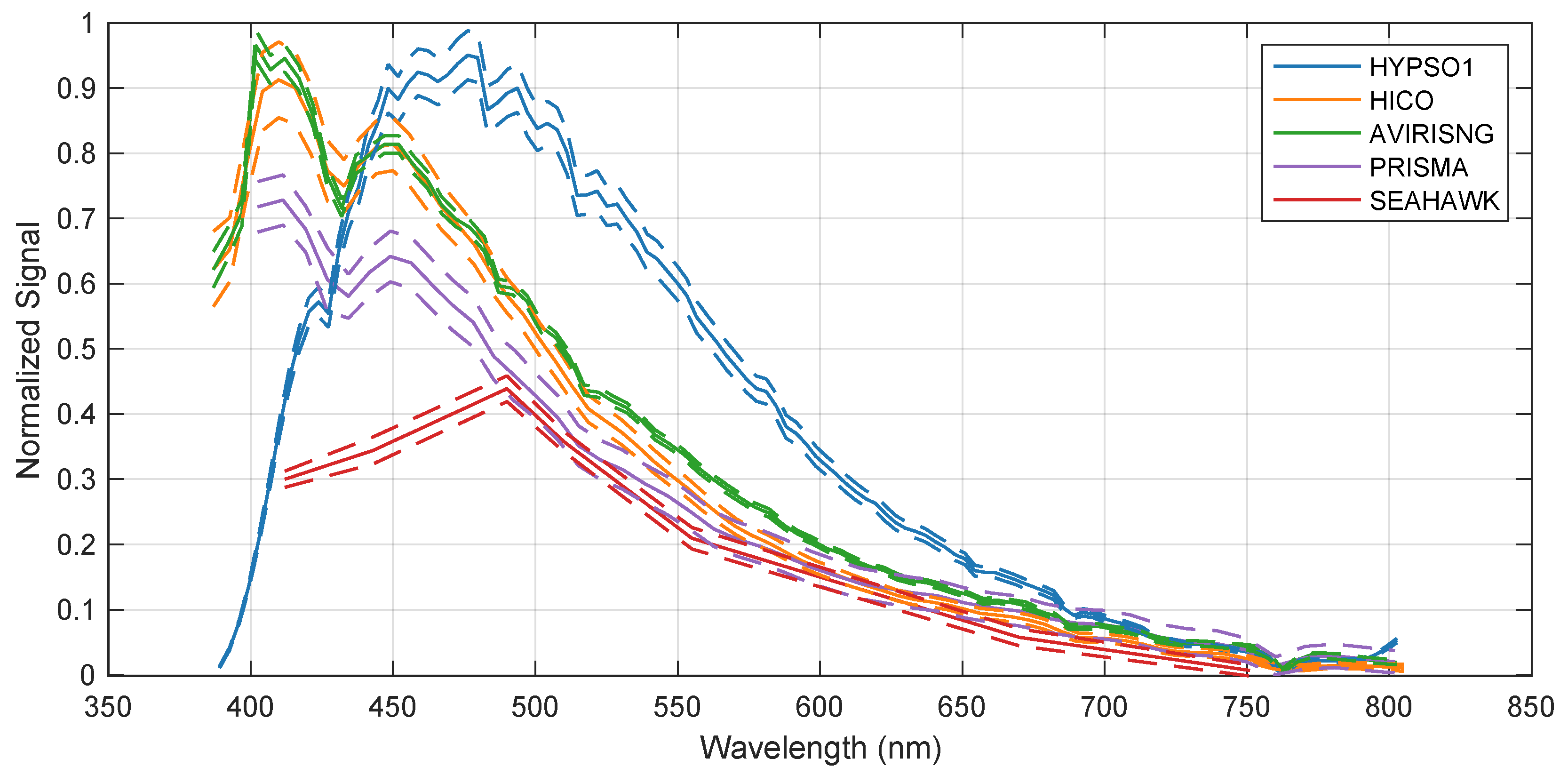
The SNR of HYPSO-1 is estimated using two different approaches and compared to four other remote sensing instruments: the multispectral 3U CubeSat–SeaHawk, Airborne Visible-Infrared Imaging Spectrometer-Next, Generation (AVIRIS-NG), PRecursore IperSpettrale della Missione Applicativa (PRISMA), and Hyperspectral Imager for the Coastal Ocean (HICO). All four sensors used for comparison produce images that have a spectral resolutions similar to HYPSO-1. The comparison only includes the spectral range that matches the HYPSO-1 payload. When interpreting the results, recall that the HYPSO-1 data are binned spectrally by summation from 1080 pixels to 120 spectral bins.
Because the data sets used do not have a ground truth, the estimated SNR characterizes the precision of the radiometric measurements and does not provide any insight concerning the accuracy of the measured signals. The results presented in this section do not attempt to compensate for the viewing and solar zenith angles of each platform during the image acquisition of the different scenes.
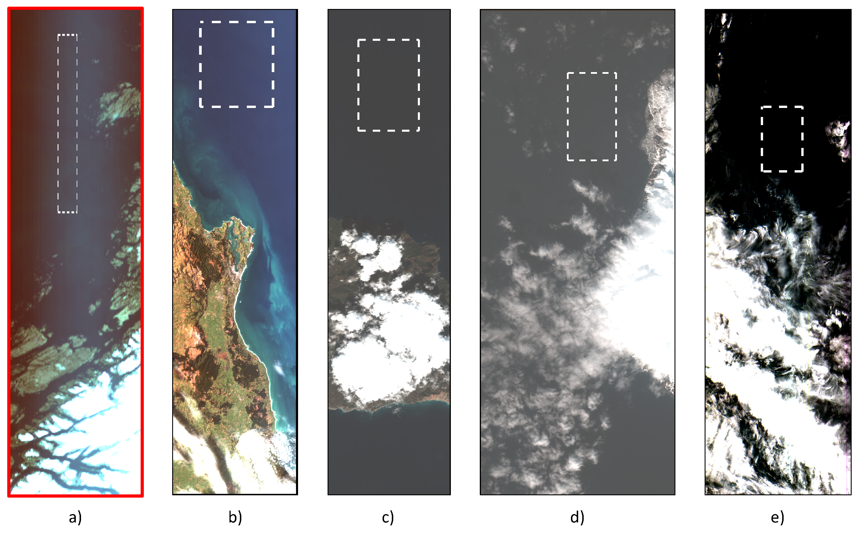
Table 8 gives relevant information on the sensors. The scenes used in this analysis are presented in
Table 9. Information on the mass of each sensor platform is added to indicate the launch cost of the respective platform. Both approaches for noise estimation are intended to be used over homogeneous areas [
28,
50,
51]. These homogeneous areas are used as the difference in the signals can be mostly attributed to sensor-level noise. The manually selected homogeneous regions of the different data sets are marked with a white dashed box in
Figure 14, while the distribution of those signals is given in
Figure 15.
Firstly, as described in [
51], the noise is estimated using an intermediate processing step of subspace identification. The underlying assumption of this method is that the radiance or reflectance at a given spectral band can be modeled by linear regression of the remaining bands. Here,
is used to denote the different spectra as matrices with each observation along the rows. Following the notation found in [
28], the noise estimation from [
51] can be performed as
Secondly, Green’s method is also used to estimate noise [
50]. The resulting noise vector set
is computed by taking the difference between neighboring pixels in a spatial area that is spectrally uniform, as follows:
These methods give a relative estimate of the SNR dependent on the statistics of a specified region of the image cube. The noise estimation is performed on raw uncalibrated data from HYPSO-1. The application of the calibration coefficient to convert the digital counts to radiance values is most commonly a linear transformation between the underlying noise and the measured signal, i.e., SNR should be unaffected by this linear scaling with these estimation approaches. Regions that appear to be homogeneous and stable, both spectrally and spatially, are selected to fit best the underlying assumptions for noise estimation, illustrated in
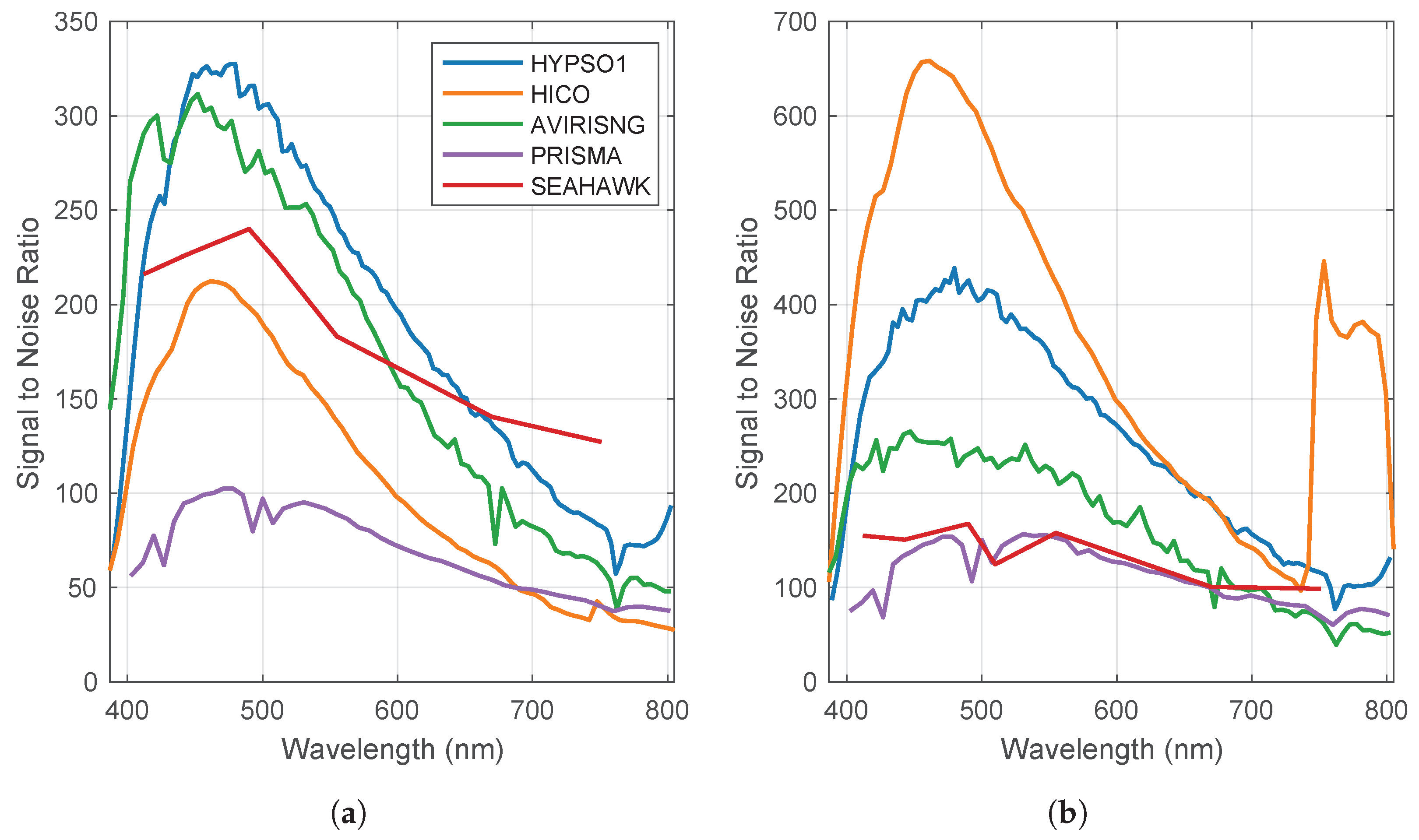
Figure 14. The results are given in
Figure 16.
The shape of the curves in
Figure 16 originates from the wavelength-dependence of water reflectance. Over water, the measured signals are mainly due to scattering in the atmosphere, and water is strongly absorbent in the longer wavelengths given in
Figure 16. In addition, the variation in the shape of the curves between sensors originates from the wavelength-dependence of the quantum efficiency, i.e., the sensor’s sensitivity to different parts of the spectrum. The SNR estimate is expected to be higher in those parts of the spectrum with the highest signal. The comparison is complex because each sensor undergoes different types of pre-processing, in addition to the variance between scenes.
The HICO data are preprocessed using a Gaussian smoothing filter. In the range of 400 nm to 745 nm, the filter size is 10 nm. For wavelengths 746 nm to 900 nm, a filter size of 20 nm is used. Data from the HICO instrument that is not preprocessed are not freely available. This preprocessing gives an artificially high SNR performance when estimated by Equation (
2). This artificially high SNR performance is evident from the counter-intuitive and significant increase in SNR from 746 nm to 900 nm, as well as the much poorer performance when estimating the noise spatially by Equation (
3). When using Equation (
3), the noise for HICO corresponds with the numbers given in [
7,
8]. This result is welcome as it supports the use of this method as an approach to estimating noise. It should also be noted that this image is from the latter part of HICO ’s operational period, and the sensor is reported to have degraded with time.
The noise estimation assumption in [
51] is unrealistic for multispectral data. As one could expect from this, Green’s method gives a better SNR performance for the multispectral SeaHawk CubeSat. The reported SNR with Green’s method does not yield as good performance as expected in the blue-green region [
19]. The SNR estimates are closer to the reported values in the longer wavelengths for SeaHawk.
The HYPSO-1 and AVIRIS-NG data fit well with the assumptions of the noise estimation models [
18,
52]. The mean acquisition elevation of the AVIRIS-NG scene is reported to be below 80 m. The sensor altitude means that the signal received is not made up of significant contributions from scattering in the atmosphere as the other sensors observe. Thus, it is reasonable to assume that the signal, or the number of photons, reaching the Focal Plane Array (FPA) is less than what is received by the other sensors. The flight path and altitude could explain why the AVIRIS-NG sensor is not performing better than the estimated SNR in
Figure 16.
The PRISMA sensor has a higher spatial resolution than the other sensors listed here [
17]. The increased spatial resolution comes at the cost of a reduced SNR for a given aperture [
7]. If one were to bin the PRISMA scene to match the spatial resolution of HICO or HYPSO-1, the SNR of PRISMA is expected to increase by a factor of
, where n is the number of bins [
7,
8,
23]. For PRISMA, this would mean a doubling of the expected SNR. However, high spatial resolution can be necessary for some operational scenarios. Furthermore, the SNR reported here is of similar shape and magnitude as reported in a previous publication regarding PRISMA’s noise characteristics over water bodies [
7]. Even though there is a difference between the two noise estimation models for the PRISMA data, both results are within the range previously reported. This result further validates the use of the noise models given here.
For the HYPSO-1 instrument, the center of the focal plane array is selected as there are fewer adverse effects from optical aberrations in this region [
24]. This choice provides an SNR that is better than what the estimates is expected to yield near the edges of the image cube. The sensor performs in line with earlier modeling [
5,
23]. As no radiometric correction or flat field corrections are applied to the data from HYPSO-1 for the SNR estimation, the assumptions in Green’s method has limited validity in the across-track direction. This dissonance should result in a poorer SNR. The homogeneous area for SNR estimation of HYPSO-1 in the across-track direction is chosen deliberately to be narrow to mitigate this limitation. Nevertheless, the SNR performance is still close to the values found in simulations [
23].
As shown in
Figure 6 in
Section 3.1, images from HYPSO-1 are slightly more blurry in terms of spatial FWHM than the ideal values proposed by [
37]. Blurring in the spatial dimensions could give an erroneous impression, given the assumptions for Green’s method. This section does not investigate whether or not this property provides any misguiding advantages in terms of the spatial SNR estimate.
The radiometric corrections discussed in
Section 3.3 can improve the SNR estimates of HYPSO-1 for the models used here. These corrections are not applied here, while the resulting SNR is still close to results from earlier simulations.
4. Discussion and Conclusions
The HYPSO-1 CubeSat has started its journey of collecting ocean color data. Observational data are planned to be made available to the scientific community as soon as the calibration and validation phase is completed, and calibrated data products can be delivered.
For nominal operations, 5–6 observations per day are possible due to mainly downlink limitations of around 450 MB per day. During campaigns, it is possible to acquire a higher number of observations, downlinking the backlog of data after each campaign as long as real-time data are not required.
Throughout the paper, we discuss the five main mission Goals, repeated here for convenience:
Goal 1: Data latency should be less than
[
25];
Goal 2: Revisit times to dedicated areas of interest should be 3–72 h [
25,
26];
Goal 3: Images should have spatial resolution better than 30–100 m per pixel [
3,
11];
Goal 4: The raw hyperspectral data should have a spectral resolution of about 5 nm or better, for VIS-NIR wavelengths [
3,
11];
Goal 5: The SNR at ToA should be greater than 400 in visual wavelengths for open ocean water [
33], and atmospherically corrected SNR of water-leaving signals should be between 40–100 [
34].
For
Goal 1, the data latency for raw data are shown to be closer to 4 h, with a single ground station. This can be significantly reduced with a ground station network, see [
15] and
Table 3 during the quick-response planning. The latency could also be reduced by using on-board processing to reduce the size of a dataset. The response time in the quick-response planning example is shown to be less than 1.5 h.
The revisit time in Goal 2 is mostly determined by the orbital properties of the satellite and the pointing constraints. Thus, the orbital period of 90 min and the location of the area of interest determine what is achievable for a given target. Targets above 60 degrees latitude (N or S) can have two consecutive passes with a 90-minute temporal separation, while targets above 70 degrees have at least three consecutive passes. Targets below 60 degrees, however, are limited to one pass per day. As small CubeSats are relatively cost-effective and scaleable, it is possible to improve revisit times by launching several.
Goal 3 is expected to be achieved in raw data with nadir pointing. The best spatial resolution in terms of GRD is estimated to be around 140 m under such conditions. Off-nadir captures increase the GRD proportionally. A higher off-nadir angle also increases the covered area. The Goal might still be achieved by significantly reducing GSD in a slewing maneuver and using super-resolution processing methods.
The in-orbit data estimate the spectral resolution to be 5.6 nm on average and 5.4 nm in the area around 600 nm, slightly exceeding the value of 5 nm in Goal 4. There is, however, room for improvement in the analysis, and further work should be carried out to estimate the spectral resolution at each spectral band.
For
Goal 5, the ToA SNR is estimated to be at least 200 for the spectral region between 450 nm and 600 nm and above 300 for important spectral regions for looking at cyanobacteria. The regions used to estimate the SNR are at the center of the FPA, and it should be stressed that this is the region of the HYPSO-1 image sensor where the observed signal is expected to be the strongest, i.e., has the best noise characteristics. With the methods for noise estimation used in
Section 3.5, the HYPSO-1 payload can deliver at the same level, or better, for certain parts of the electromagnetic spectrum, as illustrated in
Figure 16, when compared to other relevant sensors. However, from this, the Goal of SNR characteristics of the payload is not met for the ToA signal but still performs at a high level. The Goal also aims at having an SNR of at least 40 for the water leaving reflectance—that is, the signal after correcting for effects from the atmosphere’s constituents. Answering this will require investigating the performance of different algorithms and methods for compensating atmospheric effects [
7,
9]. This paper focuses on the performance of the HYPSO-1 CubeSat, its payload, and the, more or less, raw data it is acquiring. Thus, looking at different atmospheric compensation methods is beyond this paper’s scope. The atmospheric compensation of HYPSO-1 data will be a topic for future publication.
We have also demonstrated that the imaging payload can capture various image formats, depending on the desired spatial and spectral resolution and data latency. Currently, the FPGA is used exclusively for lossless image compression of the nominal cube size [
27]. In the future, with planned updates of the payload software, we aim to demonstrate how various imaging modes can improve the information throughput by using flexible onboard processing and reconfiguration the FPGA.
With the experiences from developing and operating HYPSO-1, the development of HYPSO-2 is well underway. For HYPSO-2, the Goal is to include a Software Defined Radio (SDR) that can reduce the communication latency of different platforms in the envisioned observational pyramid [
15]. The hyperspectral imaging payload will be the same concept used in HYPSO-1, with minor improvements to the optomechanical design. These improvements are made to make the platform more stable against vibrations during launch and pointing maneuvers and, as a result, improve image quality.
The HYPSO-1 CubeSat can be an important agent in a system-of-systems for monitoring oceanographic phenomena. The observational pyramid aspires to integrate measurements from several different platforms, e.g., UAVs, ASVs, and AUVs, as well as existing infrastructure for ocean color monitoring and earth observation, e.g., time-series of key environmental variables, phytoplankton biodiversity, and biomass provided by sensor buoys. This assimilation of different sensor systems should give a sounder insight into the oceanographic area of interest than the sum of their contributions.
Additional calibration and validation will be enabled by comparing data from HYPSO-1 with data from the other measurement platforms in the observational pyramid. With an operational system of systems, the collected remote sensing data will function as a feedback loop to control and correct the expected sensor degradation and other modeling limitations. The aim is that proper utilization of this feedback property can produce better and more accurate data and models for a target area over time.
The observational pyramid can be both disruptive and cost-effective infrastructure for monitoring coastal ocean and in-land water areas of interest. From the perspective of sustainable development Goals, improving this infrastructure will benefit the health and well-being of populations near the areas of interest. In addition, it will help provide clean water for drinking and sanitation, aid in the responsible consumption of aquaculture resources, guide climate action, and provide a better basis for making decisions to ensure functional ecosystems. With a functioning HYPSO-1 satellite, as reported in this paper, we are closer to reaching this Goal.


 ,
, 


