Abstract
Model error is an important source of uncertainty that significantly reduces the accuracy of El Niño–Southern Oscillation (ENSO) prediction. In this study, ensemble coupled data assimilation was employed to estimate the tendency error of the fifth-generation Lamont–Doherty Earth observation (LDEO5) model, which represented the comprehensive effect of different sources of errors. Then, the estimated tendency error was applied to an ensemble prediction system for ENSO prediction. Assimilation experiments showed that tendency error estimation yielded better analysis than state estimation only. With tendency error estimation, simulated state variables such as zonal wind stress anomalies and subsurface temperature anomalies in the Niño3.4 region and upper layer depth anomalies along the equator showed good agreement with their reanalyzed counterparts. The ensemble ENSO prediction system with tendency error estimation demonstrated significantly better prediction skill than the ensemble system without tendency error estimation or the original LDEO5 model, especially for long lead times. The tendency error estimation improved the prediction skill for El Niño more than for La Niña. This study provides a promising approach to further improve prediction skill by reducing model error effects in an ensemble prediction.
1. Introduction
The El Niño–Southern Oscillation (ENSO) is the most prominent air–sea interaction phenomenon in the tropical Pacific and has a significant global influence on the climate and weather anomalies in many regions [1]. Thus, ENSO has attracted significant attention from scientists and governments. Many efforts have been made to detect its mechanisms [2,3,4,5] and improve observations [6,7], simulations [8,9], and predictions [10,11,12]. Although research on ENSO has made significant progress over the years, many problems remain. Furthermore, ENSO prediction is a particularly important challenge [13].
Multiple statistical, dynamical, and hybrid models have been applied to ENSO prediction [10,14,15,16,17,18,19,20,21]. Overall, more than 20 models currently provide real-time forecasts of sea surface temperature (SST) anomalies in the tropical Pacific six months to one year in advance (https://iri.columbia.edu/climate/ENSO/currentinfo/update.html, accessed on 11 November 2022). However, these models still have many uncertainties. For example, most of the models gave a false alarm in predicting the 2014/2015 warm event and failed to predict the 2015/2016 very strong warm event in the tropical Pacific [20,22]. The models also show considerable variations in their forecasts, which indicate significant uncertainties.
Typically, prediction uncertainty has two types of sources: Initial errors and model errors. Studies on initial errors are abundant and mature [12,23,24]. Many studies have suggested that model errors generally play a more important role than initial errors in climate prediction [25,26]. Specifically, Zheng et al. (2009) [27] suggested that reducing model error effects could improve the ensemble ENSO prediction skill for an entire 12-month forecast, whereas the initial error mainly affects the forecast of the first few months. Thus, research on improving ENSO prediction skill has increasingly focused on reducing model error effects. Advances in atmospheric and oceanic observations have led to the wide use of data assimilation to estimate key parameters for reducing the model error effects, as well as to estimate the initial conditions for reducing initial errors [28,29]. However, this approach only estimates specific parameters, and the model errors that stem from simplified or missing physical processes remain.
Roads (1987) [30] proposed adding a constant term called the constant tendency error to the state tendency equation to represent the comprehensive effect of model errors from multiple sources. Zheng et al. (2009) [27] added stochastic model error perturbations to an ensemble ENSO prediction system to improve the prediction skill. Further studies have employed stochastic optimal perturbation to represent the stochastic atmospheric uncertainties in noise-free models and improve the ENSO prediction [12,31,32,33]. However, this approach uses state vectors and does not take advantage of observations for stochastic optimal calculation. Barkmeijer et al. (2003) [34] proposed a linear forcing singular vector to reduce the computational costs of high-dimensional systems. Duan and Zhou (2013) [35] extended the linear method to a nonlinear field and proposed the nonlinear forcing singular vector (NFSV) approach, which has been used for tendency error estimation in a series of studies on ENSO simulations and predictions [9,36,37]. The results showed that the NFSV-related model tended to have much better prediction skill than the original model. However, the NFSV algorithm requires tangent-linear and adjoint equations of the original nonlinear models, making the computations difficult and impractical in some complex dynamical models. This motivates us to consider the optimization problem of model tendency error from the framework of Bayes estimation.
Ensemble Kalman filter and its variants, such as ensemble adjustment Kalman filter (EAKF) and ensemble transform Kalman filter, are widely used as an application of Bayes estimation in atmospheric and oceanic data assimilation. These filters are mainly used for optimizing initial conditions and model parameters [12,29,38,39,40]. In this study, we attempt to solve the tendency error estimation in the framework of EAKF.
2. Materials and Methods
2.1. LDEO5 Model
The LDEO5 model is the latest version of the Zebiak–Cane (Z–C) model, which is a famous ocean–atmosphere-coupled model covering the tropical Pacific Ocean [14,41,42]. The LDEO5 model is widely used for ENSO simulation and prediction [10,43,44]. We described the model in our previous paper [12] but summarize it here as follows. The atmospheric dynamics, covering the domain of 101.25°E–286.875°E and 29°S–29°N with the grid spacing of 5.625° (longitude)×2° (latitude), are governed by steady-state and linear shallow-water equations [45], which simulate the wind response to heating anomalies parameterized by SST anomalies. The oceanic dynamics, covering the domain of 125°E–281°E and 28.75°S–28.75°N with a grid spacing of 2° (longitude) × 0.5° (latitude), are simulated using a reduced-gravity model, which is forced by wind stress anomalies from the atmospheric model. The oceanic thermodynamics, covering the domain of 129.375°E–275.625°E and 19°S–19°N with the same grid as that of atmospheric model, are modeled by a three-dimensional nonlinear equation for SST anomalies:
where denotes an SST anomaly, and and represent the monthly means of the SST and vertical temperature gradient, respectively. and represent horizontal and upwelling current velocity anomalies, respectively, and and represent their climatological values, respectively. represents the subsurface entrainment temperature anomaly, and denotes the depth of the surface layer of the ocean. when , which means that only the upwelling current velocity is considered in Equation (1). The model time step is 10 days. More details about the Z–C model can be found in Zebiak and Cane (1987) [14].
With regard to the prediction of SST anomalies by the LDEO5 model, the SST tendency error can be attributed to the comprehensive effects of the model errors. Thus, we can superimpose an external forcing in Equation (1) to offset the model error effects. Based on this idea, the developmental equation for SST anomalies can be written as:
where denotes model tendency error, and denotes the time step of LDEO5 model.
2.2. Ensemble Adjustment Kalman Filter
We employed the EAKF for data assimilation [46,47]. For a single observation, EAKF analysis can be divided into three steps. The first step is to compute the observational increment, which can be expressed as:
where denotes the projection of the th member for the model states into observational space with an ensemble mean of and variance of , and denotes the observation with a variance of . The second step is to project the observational increment in observational space onto related model variables in model space, based on the following linear regression:
where denotes the contribution of to the model variable for the th member. denotes the error covariance between the prior state ensemble of and projected state ensemble of . The third step is to analyze (i.e., update) the state variable:
where and represent the th member of the prior state variable before analysis and posterior state variable after analysis, respectively. The procedure iterates with each individual observation in sequence until all observations are assimilated. As we will mention later, the updated variable here is an SST anomaly, since the observation to be assimilated and the state variable to be adjusted are both SST anomalies. Figure 1 shows a flowchart of data assimilation based on EAKF.
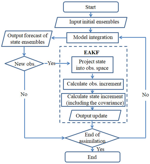
Figure 1.
Flowchart of the data assimilation based on EAKF.
With a crossing or coupling error covariance, EAKF can naturally implement multivariate increments [28]. For instance, with cross-correlations, parameters can easily be estimated through a state augmentation technique [40,48,49]. In this study, the model tendency error (i.e., can be treated as a parameter. Therefore, tendency error estimation can be referred to as parameter estimation. Notably, the tendency error superimposed into the SST anomalies equation is different from the intrinsic parameters of the LDEO5 model, which have their reference values. At each step of data assimilation, the observational increment is also linearly projected to the increment of :
where denotes the error covariance between the prior tendency error ensemble of and projected state ensemble of . The analysis of is given by:
where and represent the th member of prior and posterior tendency error, respectively. With this procedure, can be estimated by EAKF.
The quality of the tendency error estimation mainly depends on the accuracy of the error covariance between the tendency error and projection for model states. To effectively enhance the accuracy of the error covariance, the coupled data assimilation scheme for enhancive parameter correction (DAEPC) proposed by Zhang et al. (2012) [50] was employed in this study. Within DAEPC, the tendency error is estimated after the state estimation reaches a quasi-equilibrium, such that the uncertainty of model states can be sufficiently constrained by observations.
2.3. Data
The observation to be assimilated were monthly Kaplan SST anomalies [51]. The dataset provides monthly SST anomalies with temporal coverage from January 1856 to the present and spatial coverage of the 5.0° latitude by 5.0° longitude global region (2.5°E–357.5°E, 87.5°S–87.5°N). The data used in this study are monthly SST anomalies from January 1856 to December 2021 covering the tropical Pacific (the region of 97.5°E–287.5°E, 32.5°S–32.5°N). Before assimilation, the monthly Kaplan SST anomalies were first processed by space–time smoothing and then interpolated into the grids of the LDEO5 model.
Among the variables in the LDEO5 model, the assimilated variable of SST anomalies was used to evaluate directly the assimilation effect. Other key state variables of the zonal wind stress (ZWS), upper layer depth (ULD), and subsurface temperature (Te) anomalies were used to evaluate indirectly the effect of the assimilation system on the simulation ability of the LDEO5 model. The referenced ZWS anomalies are calculated from the wind speed of the first atmospheric reanalysis of the 20th century (ERA-20C) of the European Centre for Medium-Range Weather Forecasts, which ranges from January 1900 to February 2010 for the region of 0–358.875°E, 89.1415°S–89.1415°N with a resolution of 1.125° latitude by about 1.125° longitude [52]. The wind-speed data covering the tropical Pacific (the region of 101.25°E–286.875°E, 29.7195°S–29.7195°N) should be converted to ZWS anomalies before using them in this study. The referenced ULD and Te anomalies are both calculated from the temperature of simple ocean data assimilation (SODA) reanalysis [53,54], which provides the reanalysis of oceanic and air–sea interface data covering the region of 0.25°E–359.75°E, 75.25°S–89.25°N with a resolution of 0.5°. The used temperature covers the region of 129.25°E–275.75°E, 19.25°S–19.25°N with temporal coverage from January 1980 to December 2015 in this study.
2.4. Experiments
We first performed a data assimilation experiment based on a coupled data assimilation system using EAKF. We then used the results of the data assimilation experiments for ensemble ENSO prediction.
Three assimilation schemes were compared. First, EAKF_F-Assim assimilated the monthly Kaplan SST anomalies over the tropical Pacific using the EAKF method to update SST anomalies and . For simplicity, we assumed is constant and geography independent. Second, EAKF-Assim only updated SST anomalies (i.e., state estimation only) to highlight the effect of tendency error estimation. Similarly, we used the assimilation scheme of Chen et al. (2004) [10], which is a single assimilation and updates only SST anomalies by replacing them with observed ones to highlight the effect of EAKF. This scheme is parallel to the other two EAKF schemes; thus, we called it “Ori-Assim”. For fair comparison, the three assimilation schemes were set to the same assimilation frequency of once per month. The settings of the assimilation experiment are summarized in Table 1.

Table 1.
Settings of the assimilation experiment.
For EAKF-Assim and EAKF_F-Assim, we assumed that the observational error variance was 0.25 °C [51]. The covariance inflation approach [55] was employed to prevent filter divergence because of an underestimated ensemble spread. For simplicity, we employed multiplicative inflation with a fixed factor:
where denotes the th member of a state variable before inflation with an ensemble mean of , denotes the th member of the inflated state variable, and denotes a fixed inflation factor. Inflation can be divided into three categories depending on what the inflation factor acts on: prior inflation (i.e., the prior variable is inflated), posterior inflation (i.e., the posterior variable is inflated), and hybrid inflation (i.e., the prior and posterior variables are both inflated) [56]. For state inflation, we employed posterior inflation after evaluating the performances with all three categories. Inflation factors with a range of 1.0–1.4 were tested at intervals of 0.05 in EAKF-Assim, and a value of 1.2 achieved the best results. As a contrast, we used the same inflation factor (i.e., 1.2) for state estimation in EAKF_F-Assim, while for tendency error estimation, we tested a range of 1.0–1.2 at intervals of 0.01 and found a value of 1.01 achieved the best results.
To reduce the spurious correlation between model states and remote observations, a covariance localization scheme was used in EAKF-Assim and EAKF_F-Assim. We employed the Gaspari−Cohn function [57] to cut off long-distance correlations:
where represents the distance between the model grid and observational location, and defines the localization parameter used for decorrelation. In practice, the localization factor when . With increasing distance, decreases gradually until for . After a series of tests, we set the decorrelation length to four times the distance between adjacent grids for both EAKF-Assim and EAKF_F-Assim.
To reduce computational costs, both EAKF-Assim and EAKF_F-Assim were set to an ensemble size of 30. The initial perturbations of SST anomalies were represented as random numbers in a Gaussian distribution with a mean of zero and variance of 1 °C. Obtaining the initial perturbations of tendency error remains an issue that will be discussed later. To ensure a quasi-equilibrium state in EAKF_F-Assim, the tendency error estimation was activated after five years of state estimation only.
As mentioned in Section 2.3, the variables in the LDEO5 model in the assimilation experiment (i.e., SST, ZWS, ULD, and Te anomalies), constitute the initial conditions for ENSO prediction. Only EAKF_F-Assim provided the tendency error estimation. Table 2 presents the three schemes considered in the ENSO prediction experiment: Ori-Pred, EAKF-Pred, and EAKF_F-Pred. The prediction experiment covered the period of January 1856–December 2021. Each forecasting lasted for 12 months and was initialized from the beginning of each month. EAKF_F-Pred used the analysis of at each assimilation step for each forecast.
Table 2.
Settings of the prediction experiment.
3. Results
The Kaplan SST anomalies in January 1856 provided the initial guess of SST anomalies for EAKF. The initial ensembles of SST anomalies were obtained with Gaussian perturbations added to the initial guess. However, there were no actual observations that could be used for the tendency error, and it is not an inherent parameter of the Z–C model. Therefore, the initial ensemble of the tendency error for EAKF_F-Assim needed to be determined before the assimilation experiment. Because the tendency error represents the comprehensive effect of model errors, it is natural to assume that the analysis errors in SST anomalies in EAKF-Assim can be used as its reference value. Note that the analysis errors are calculated by the differences between the values after assimilation in EAKF-Assim and the monthly Kaplan SST anomalies. Figure 2 shows the time-varying analysis errors in SST anomalies in EAKF-Assim. There was an initial shock for the first years of assimilation, which is why we adopted DAEPC. Moreover, the analysis errors over most decades oscillated within a range of −0.2 °C to 0.2 °C with an average of −0.0019 °C. We randomly selected 30 analysis errors in SST anomalies in EAKF-Assim for the period of 1856–2021 as the initial ensemble of tendency errors.
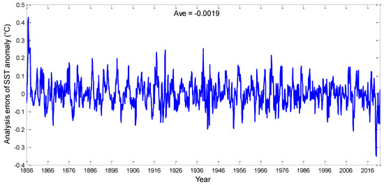
Figure 2.
Time-varying analysis errors of SST anomalies in EAKF-Assim.
3.1. Data Assimilation Analysis
Figure 3 shows the temporal evolution of the ensemble spread and analysis of with the assimilation length for EAKF_F-Assim. The ensemble spread and analysis of remained constants for the first 5 years because there was no tendency error estimation. After the tendency error estimation was activated, the ensemble spread declined rapidly and then maintained a certain magnitude, which indicates that the filter was effective. Meanwhile, the analysis of first oscillated and then converged to a relatively steady value of about −0.003, which is the same order of magnitude as that of the average for the initial tendency error, (i.e., the average of analysis errors as shown in Figure 2). These results suggest that the tendency error estimation somewhat compensated for deviations in the model simulation.
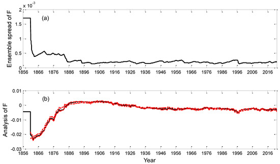
Figure 3.
Temporal evolution of the (a) ensemble spread and (b) analysis of in EAKF_F-Assim. The black line in (b) represents the average of the ensemble members, and the two red dashed lines are the maximum and minimum members.
To validate the assimilation performance of EAKF_F-Assim, the analysis of state variables needed to be evaluated. Figure 4 shows the time series of the ensemble spread and root mean square (RMS) errors of Niño3.4 SST anomalies (the averaged SST anomalies over the Niño3.4 region, which is defined by the region of 190°E–240°E, 5°S–5°N) before and after assimilation with EAKF_F-Assim. The order of magnitude of ensemble spread was the same as that of the observational error variance, both of which were . The result indicates that the filter worked throughout the assimilation. The time-averaged RMS error after assimilation was 0.1913, which is significantly lower than the error of 0.2958 before assimilation. This further suggests the positive effect of data assimilation.
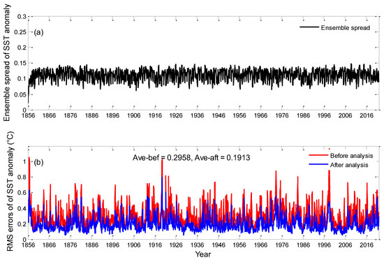
Figure 4.
Time series of the (a) ensemble spread and (b) RMS errors of Niño3.4 SST anomalies before and after assimilation in EAKF_F-Assim.
Additionally, we also evaluated the ability of three schemes to simulate other state variables: the ZWS, ULD, and Te anomalies. Figure 5 shows the time series of ZWS anomalies averaged over the Niño3.4 region from the ERA-20C reanalysis and the amplitude simulated by Ori-Assim, EAKF-Assim, and EAKF_F-Assim. The correlation coefficients between the reanalysis and simulation from Ori-Assim, EAKF-Assim, and EAKF_F-Assim were 0.6809, 0.7283, and 0.7334, respectively, while the RMS errors from Ori-Assim, EAKF-Assim, and EAKF_F-Assim were 0.0797 dy/cm2, 0.0681 dy/cm2, and 0.0617 dy/cm2, respectively.
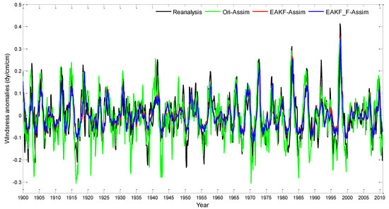
Figure 5.
Time series of ZWS anomalies in the Niño3.4 region: ERA-20C reanalysis and simulations from Ori-Assim, EAKF-Assim, and EAKF_F-Assim schemes in black, green, red, and blue lines, respectively.
Figure 6 shows the time–longitude diagrams of the ULD anomalies over the equatorial region from SODA reanalysis and the simulations from the three schemes. Generally, the simulations from three schemes captured the key characteristics such as the thermocline variability and eastward propagation. Additionally, the amplitude simulated by Ori-Assim was significantly greater than that from the reanalysis and from other two schemes. The correlation coefficients between the reanalysis and simulation from Ori-Assim, EAKF-Assim, and EAKF_F-Assim were 0.6865, 0.7153, and 0.7377, respectively, while the RMS errors from Ori-Assim, EAKF-Assim, and EAKF_F-Assim were 10.6159 cm, 7.9461 cm, and 7.0761 cm, respectively. EAKF_F-Assim achieved the best simulation of ULD anomalies.
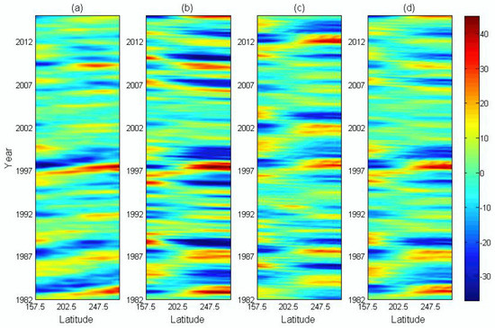
Figure 6.
Time–longitude diagrams of ULD anomalies over the equatorial region: (a) SODA reanalysis and simulations from (b) Ori-Assim, (c) EAKF-Assim, and (d) EAKF_F-Assim schemes.
ENSO phase evolution is mainly dominated by the subsurface thermal variation. Figure 7 shows the evolution of Te anomalies averaged over the Niño3.4 region from SODA reanalysis and simulations from the three schemes. The correlation coefficient between the reanalysis and simulation from Ori-Assim, EAKF-Assim, and EAKF_F-Assim was 0.6118, 0.7589, and 0.7631, respectively, while the RMS errors from Ori-Assim, EAKF-Assim, and EAKF_F-Assim were 0.8581 °C, 0.8133 °C, and 0.7852 °C, respectively. Similar to the results of ZWS and ULD anomalies, EAKF_F-Assim got the best simulation of the subsurface thermal variability.
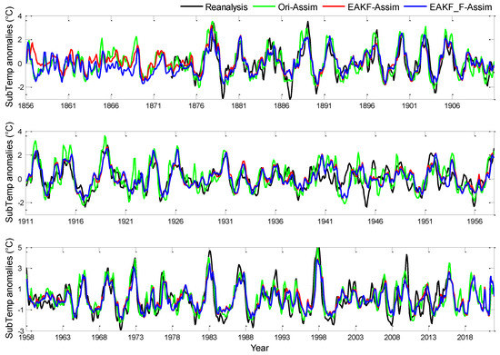
Figure 7.
Evolution of Te anomalies averaged over the Niño3.4 region: SODA reanalysis and simulations from Ori-Assim, EAKF-Assim, and EAKF_F-Assim schemes in black, green, red, and blue lines, respectively.
To verify the significance of difference among different experiments, a statistical method is used in this study. Bootstrap is a statistical method that can be used to place confidence intervals on data ensembles. It involves multiple resampling from one’s own data to create a series of bootstrap samples of the same size. If the bars consisting of maximum and minimum values of multiple resampling among experiments are non-overlapping, the difference is significance. After analysis of the bootstrap samples, the variation among the resulting estimates is used to indicate the uncertainty of the original data ensembles. We used this approach to test the significance of the difference between EAKF_F-Assim and EAKF-Assim in Figure 5, Figure 6 and Figure 7, and the results indicate that the difference is not statistically significant.
Figure 8 shows the time series of the observed and analyzed Niño3.4 SST anomalies with the three schemes. All three schemes showed good agreement with the observed values. As described by Chen et al. (2004) [10], Ori-Assim replaces the modeled SST anomalies with the observed counterparts, so the correlation coefficient was 1.0000. EAKF_F-Assim had a correlation coefficient of 0.9576, which is larger than that of EAKF-Assim. Thus, the analysis of SST anomalies was better with a tendency error estimation than that without it, which indicates that tendency error estimation has a positive effect on the analysis of SST anomalies. The bootstrap method was used to test the significance of difference between the analyzed Niño3.4 SST anomalies from the EAKF-Assim and EAKF_F-Assim schemes. The results show that the difference is significant statistically (not shown here).
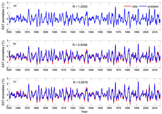
Figure 8.
Time series of observed (red) and analyzed (blue) Niño3.4 SST anomalies: (a) Ori-Assim, (b) EAKF -Assim, and (c) EAKF_F-Assim schemes.
3.2. ENSO Predictions
We demonstrated in a previous paper [12] that Ori-Assim provided the best analysis of SST anomalies (i.e., best initial conditions in term of SST anomalies) but led to the worst ENSO prediction. In this study, we evaluated the effect of tendency error estimation on ENSO prediction. To evaluate the overall ENSO prediction skill, we employed two quantities: the anomaly correlation coefficient (ACC) and RMS error of the forecasted ensemble mean of the Niño3.4 index relative to the observations. The ACC and RMS error for the th leading months are given by:
where represents the number of predictions in the experiment, which was equal to (155 years (1866 to 2020) with 12 predictions per year) in this study. The results of the first 10 years were eliminated because this period suffered from the initial shocks for the SST anomalies and tendency error. denotes the ensemble mean of forecasted SST anomalies with a mean of over the Niño3.4 region, and denotes the observational counterpart with a mean of .
Figure 9a,b show the ACCs and RMS errors, respectively, between the observed and forecasted Niño3.4 SST anomalies with respect to the lead time in months. The results for persistence as reference are also plotted. We found that the three prediction experiments are much more skillful than persistence. Among the three prediction experiments, EAKF_F-Pred showed the best prediction skill, which was followed by EAKF-Pred and Ori-Pred. If we define the valid lead time using an ad hoc value of 0.6 for the ACC, tendency error estimation extended the valid lead time by 1 month compared to original scheme. The prediction skill of EAKF-Pred was between that of Ori_Pred and EAKF_F-Pred, which indicates that tendency error estimation improved prediction skill. We used the bootstrap method to verify the significance of difference between EAKF-Pred and EAKF_F-Pred. The error bars in Figure 9a represent the sampling errors (measured by the maximum and minimum values of multiple resampling) with different lead times. For the first few months of lead time, the difference between the ACCs of EAKF-Pred and EAKF_F-Pred was not statistically significant. With a longer lead time, EAKF_F-Pred showed a significantly better ACC than EAKF-Pred based on the statistical analysis. This confirms Zheng et al.’s (2009) conclusion that considering the model error effect could improve the ensemble prediction skill for the entire forecast process, especially with long lead times [27].
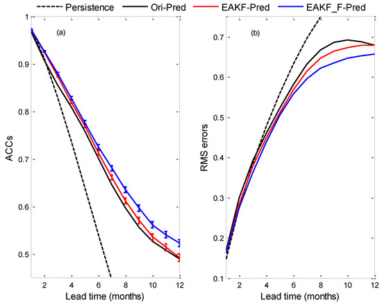
Figure 9.
(a) ACCs and (b) RMS errors between observed and forecasted Niño3.4 SST anomalies with respect to the leading months in persistent prediction and three prediction experiments.
It is noteworthy that the original scheme produced the best SST anomaly analyses but the worst prediction skill. This is because the initial conditions include not only an SST anomaly but also other variables, such as the ZWS and ULD anomalies. Unfortunately, the original scheme had the worst simulations of ZWS and ULD anomalies as shown in Section 3.1, leading to a dynamic and physical imbalance in the initial conditions [58]. In addition, the SST anomalies and other variables in EAKF_F-Pred are better than those in EAKF-Pred; as a result, the prediction skill in the former is better than that in the latter. This is because the tendency error estimation not only makes the dynamics and physics more balanced in the initial conditions, but also reduces the errors of the forecast model.
To assess the impact of tendency error estimation on ENSO prediction, Figure 10a,c show the time series (1866–2021) of observed and forecast Niño3.4 SST anomalies using EAKF_F-Pred with a lead time of 6 months. The forecasts fit the observations sufficiently well. The correlation coefficient was about 0.73 up to a lead time of 6 months, which is comparable with the state of the art [17,59,60]. Moreover, most strong El Niño events (defined as the Niño3.4 SST anomaly greater than 1.0 °C, as in Chen et al. [10]) were predicted successfully at a lead time of 6 months, which indicates that tendency error estimation can predict the intensities of most warm events. However, the prediction of strong cold events (defined as the Niño3.4 SST anomaly being smaller than −1.0 °C, as in Chen et al. [10]) showed some deviation. Figure 10b,d show the time series of absolute errors (AEs) of forecasted SST anomalies in the Niño3.4 region using EAKF_F-Pred with a lead time of 6 months. The results for EAKF-Pred are also plotted as a reference. Overall, EAKF_F-Pred had lower AEs than EAKF-Pred, and the reductions were mainly during warm events. Specifically, the time-averaged AEs decreased from about 0.43 °C with EAKF-Pred to about 0.35 °C with EAKF_F-Pred. The bootstrap test showed that the difference between the AEs of forecasted Niño3.4 SST anomalies using EAKF-Pred and EAKF_F-Assim schemes is significant statistically for most large events (not shown here).
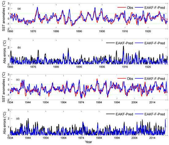
Figure 10.
Time series of (a,c) observed and forecasted Niño3.4 SST anomalies using EAKF_F-Pred with a lead time of 6 months, and (b,d) AEs of forecasted Niño3.4 SST anomalies using EAKF-Pred and EAKF_F-Assim schemes with a lead time of 6 months.
To confirm the above results, we investigated the prediction for warm and cold events separately. First, a strong El Niño was defined as when the Niño3.4 index was greater than 1 °C, whereas a strong La Niña was defined as when the Niño3.4 index was less than −1 °C [10]. Then, composites of strong El Niño and strong La Niña events were computed with the observations, as shown in Figure 11a,b, respectively. Finally, the AEs of the predicted composites of the two types of events using EAKF-Pred and EAKF_F-Assim with a lead time of 6 months were computed, as illustrated in Figure 11c–f. For the composite strong El Niño, EAKF-Pred showed large forecast errors of SST anomalies over the tropical Pacific south of the equator. The region-averaged AE was 0.73 °C. These errors were reduced by EAKF_F-Pred with a region-averaged value of 0.57 °C. For the composite strong La Niña, EAKF_F-Pred generated lower AEs with a region-averaged value of 0.65 °C over the central Pacific than EAKF-Pred with 0.75 °C. In summary, tendency error estimation significantly improved the prediction for El Niño but not for La Niña, which is consistent with the above conclusions. The bootstrap test showed that the improvements for the two flavor events are significant statistically (not shown here).
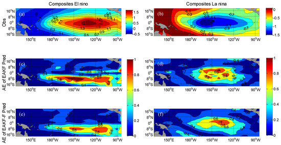
Figure 11.
Composite (a) El Niño and (b) La Niña calculated from observations. AEs of the predicted composite (c) El Niño and (d) La Niña using EAKF-Pred with a lead time of 6 months. AEs of the predicted composite (e) El Niño and (f) La Niña using EAKF_F-Pred with a lead time of 6 months.
4. Discussion
The model error is an important source of uncertainty in ENSO prediction. Thus, reducing the model error effect is essential to improving the prediction ability of climate models. Because this study was a preliminary application of tendency error estimation with ensemble coupled data assimilation, the tendency error was assumed a constant in space. However, the tendency error should actually be a local state-dependent variable, which is similar to an intrinsic model parameter [61,62]. We believe that geography-dependent tendency error estimation will further reduce the model error effect and thus improve the ENSO prediction skill, and this is currently under research.
Covariance inflation is widely used to address filter divergence caused by variance underestimation [52,63]. In the present study, we employed multiplicative posterior inflation with fixed factors to deal with filter divergence. However, some adaptive inflation algorithms have achieved success in the fields of atmosphere and ocean sciences [64,65,66,67]. Further studies on applying adaptive inflation to tendency error estimation are still required.
In the ensemble prediction experiment, the tendency error is estimated at the current assimilation step. This raises the question of how real forecasts can be carried out without future observations. Tao and Duan (2019) [37] first predetermined a function of NFSV-tendency errors as the observed initial SST anomalies, and then derived a tendency error forecast model. They coupled the forecasted NFSV-tendency error with a climate model to establish an ENSO prediction system. In our study, numerous experiments showed that the estimated tendency error was closely related to the initial SST anomalies. For instance, we performed ensemble assimilation and prediction experiments for the period of January 1980–December 2021 (not shown here). Although the estimated tendency error was different from that for the period of January 1856–December 2021 in this study, EAKF_F-Pred demonstrated a robust ENSO prediction skill. Thus, this study provides a promising foundation for reducing model error effects and improving the ENSO prediction skill of climate models. In the next study, we will focus on performing real predictions without future observations.
5. Conclusions
In this study, we defined the comprehensive effect of model errors in the LDEO5 model as the SST tendency error and then estimated it using an EAKF-based coupled data assimilation system for the period of January 1856−December 2021. The tendency error was estimated with SST anomalies simultaneously using the Kaplan SST anomalies. The data assimilation experiment indicated that estimating the tendency error (i.e., EAKF_F-Assim) yielded better results for the SST anomaly analysis than state estimation only (i.e., EAKF-Assim). Modeled state variables (e.g., ULD anomalies along the equator, ZWS anomalies, and Te anomalies in the Niño3.4 region) in EAKF_F-Assim achieved the best agreement with their reanalyzed counterparts among the three schemes. Ensemble ENSO predictions were carried out using the data assimilation results for the initial conditions. EAKF_F-Pred demonstrated a significantly higher prediction skill than EAKF-Pred and Ori-Pred, especially for long lead times. Tendency error estimation improved the prediction skill more for El Niño than La Niña.
The above results were based on a randomly selected initial ensemble of tendency errors. To rule out the influence of randomness, we performed multiple randomized trials. Although the results of each randomized trial were somewhat different, the conclusions were consistent: tendency error estimation reduced model error effect s and improved the ENSO prediction skill, especially for long lead times, and the improvement in prediction was greater for El Niño than La Niña. This study provides a promising approach to further improve prediction skill by reducing model error effects in an ensemble prediction.
Author Contributions
Conceptualization, Y.G. and Y.T.; formal analysis, Y.G.; funding acquisition, Y.T. and Y.G.; methodology, Y.G. and Y.T.; software, Y.G. and T.L.; validation, Y.G. and Y.T.; writing, Y.G. and Y.T. All authors have read and agreed to the published version of the manuscript.
Funding
This work was jointly supported by the National Natural Science Foundation of China (42227901, 42130409), Southern Marine Science and Engineering Guangdong Laboratory (Zhuhai) (Grant No. SML2021SP314), Scientific Research Fund of the Second Institute of Oceanography, MNR (Grant No. JG1809), and Innovation Group Project of Southern Marine Science and Engineering Guangdong Laboratory (Zhuhai) (Grant No. 311021009).
Data Availability Statement
In addition to the assimilation and reanalysis data presented in the text, the prediction data are available at the Second Institute of Oceanography, Ministry of Natural Resources, China. Further inquiries can be directed to the corresponding author.
Acknowledgments
We are very thankful to D. Chen for providing the code of the latest version of the Z-C model. We are very thankful to X. Song and Z. Shen for their guidance on the code of EnKF. We thank the anonymous reviewers for their useful and careful comments on the manuscript.
Conflicts of Interest
The authors declare no conflict of interest.
References
- McPhaden, M.J.; Zebiak, S.E.; Glantz, M.H. ENSO as an integrating concept in earth science. Science 2006, 314, 1740–1745. [Google Scholar] [CrossRef] [PubMed]
- Wyrtki, T. El Nino–the dynamic response of equatorial Pacific Ocean to atmospheric forcing. J. Phys. Oceanogr. 1975, 5, 572–583. [Google Scholar] [CrossRef]
- Philander, S.G.; Yamagata, T.; Pacanowski, R.C. Unstable air-sea interactions in the tropica. J. Atmos. Sci. 1984, 41, 604–613. [Google Scholar] [CrossRef]
- Suarez, M.J.; Schopf, P.S. A delayed action oscillator for ENSO. J. Atmos. Sci. 1988, 5, 3283–3287. [Google Scholar] [CrossRef]
- Jin, F.F. An equatorial ocean recharge paradigm for ENSO. Part I: Conceptual model. J. Atmos. Sci. 1997, 54, 811–829. [Google Scholar] [CrossRef]
- Trenberth, K.E.; Branstator, G.W.; Karoly, D.; Kumar, A.; Lau, N.C.; Ropelewski, C. Progress during TOGA in understanding and modeling global teleconnections associated with tropical sea surface temperatures. J. Geophys. Res. 1998, 103, 14291–14324. [Google Scholar] [CrossRef]
- Wallace, J.M.; Rasmusson, E.M.; Mitchell, T.P.; Kousky, V.E.; Sarachik, E.S.; von Storch, H. On the structure and evolution of ENSO-related climate variability in the tropical pacific: Lessons from TOGA. J. Geophys. Res. 1998, 103, 14241–14259. [Google Scholar] [CrossRef]
- Kug, J.S.; Ham, Y.G.; Lee, J.Y.; Jin, F.F. Improved simulation of two types of El Niño in CMIP5 models. Environ. Res. Lett. 2012, 7, 034002. [Google Scholar] [CrossRef]
- Duan, W.S.; Tian, B.; Xu, H. Simulations of two types of El Niño events by an optimal forcing vector approach. Clim. Dyn. 2014, 43, 1677–1692. [Google Scholar] [CrossRef]
- Chen, D.K.; Cane, M.A.; Zebiak, S.; Huang, D.J. Predictability of El Niño over the past 148 years. Nature 2004, 428, 733–736. [Google Scholar] [CrossRef]
- Tao, L.J.; Gao, C.; Zhang, R.H. Model parameter-related optimal perturbations and their contributions to El Niño prediction errors. Clim. Dyn. 2019, 52, 1425–1441. [Google Scholar] [CrossRef]
- Gao, Y.Q.; Liu, T.; Song, X.S.; Shen, Z.Q.; Tang, Y.M.; Chen, D.K. An extension of LDEO5 model for ENSO ensemble predictions. Clim. Dyn. 2020, 55, 2979–2991. [Google Scholar] [CrossRef]
- Zhang, S.Q. Coupled data assimilation and parameter estimation in coupled ocean–atmosphere models: A review. Clim. Dyn. 2020, 54, 5127–5144. [Google Scholar] [CrossRef]
- Zebiak, S.E.; Cane, M.A. A model El Niño–southern oscillation. Mon. Wea. Rev. 1987, 115, 2262–2278. [Google Scholar] [CrossRef]
- Latif, M.; Anderson, D.; Barnett, T.; Cane, M.; Kleeman, R.; Leetmaa, A.; O’Brien, A.; Rosati, E.; Schneider, E. A review of the predictability and prediction of ENSO. J. Geophys. Res. 1998, 103, 14375–14393. [Google Scholar] [CrossRef]
- Tang, Y.M.; Hsieh, W.W. Hybrid coupled models of the tropical pacific–ENSO prediction. Clim. Dyn. 2002, 19, 343–353. [Google Scholar] [CrossRef]
- Barnston, A.G.; Tippett, M.K.; L’Heureux, M.L.; Li, S.H.; DeWitt, D.G. Skill of real-time seasonal ENSO model predictions during 2002-11: Is our capability increasing? Bull. Am. Meteorol. Soc. 2012, 93, 631–651. [Google Scholar] [CrossRef]
- Tippett, M.K.; Barnston, A.G.; Li, S.H. Performance of recent multi-model ENSO forecasts. J. Appl. Meteorol. Clim. 2012, 51, 637–654. [Google Scholar] [CrossRef]
- Zhang, R.H.; Gao, C. The IOCAS intermediate coupled model (IOCAS ICM) and its real-time predictions of the 2015-16 El Niño event. Sci. Bull. 2016, 66, 1061–1070. [Google Scholar] [CrossRef]
- Luo, J.J.; Wang, G.; Dommenget, D. May common model biases reduce CMIP5’s ability to simulate the recent Pacific La Niña-like cooling? Clim. Dyn. 2018, 18, 1335–1351. [Google Scholar] [CrossRef]
- Zhang, R.H.; Yu, Y.Q.; Song, Z.Y.; Ren, H.L.; Tang, Y.M.; Qiao, F.L.; Wu, T.; Gao, C.; Hu, J.; Tian, F.; et al. A review of progress in coupled ocean-atmosphere model developments for ENSO studies in China. J. Oceanol. Limnol. 2020, 38, 930–961. [Google Scholar] [CrossRef]
- Lian, T.; Chen, D.K.; Tang, Y.M. Genesis of the 2014–2016 El Niño events. Sci. China: Earth Sci. 2017, 60, 1589–1600. [Google Scholar] [CrossRef]
- Mu, M.; Xu, H.; Duan, W.S. A kind of initial errors related to “spring predictability barrier” for El Niño events in Zebiak-Cane model. Geophys. Res. Lett. 2007, 34, L03709. [Google Scholar] [CrossRef]
- O’Kane, T.J.; Sandery, P.A.; Monselesan, D.P.; Sakov, P.; Stevens, L. Coupled data assimilation and ensemble initialization with application to multiyear ENSO prediction. J. Clim. 2019, 32, 997–1024. [Google Scholar] [CrossRef]
- Latif, M.; Sperber, K.; Arblaster, J.; Braconnot, P.; Chen, D.; Colman, A.; Cusbach, U.; Cooper, C.; Delecluse, P.; Dewitt, D.; et al. ENSIP: The El Niño simulation intercomparison project. Clim. Dyn. 2001, 18, 55–276. [Google Scholar] [CrossRef]
- Stainforth, D.A.; Aina, T.; Christensen, C.; Collins, M.; Faull, N.; Frame, D.J.; Kattleborough, J.A.; Knight, A.; Martin, A.; Murphy, J.M.; et al. Uncertainty in predictions of the climate response to rising levels of greenhouse gases. Nature 2005, 433, 403–406. [Google Scholar] [CrossRef]
- Zheng, F.; Wang, H.; Zhu, J. ENSO ensemble prediction: Initial error perturbations vs. model error perturbations. Chin. Sci. Bull. 2009, 54, 2516–2523. [Google Scholar] [CrossRef]
- Wu, X.R.; Han, G.J.; Zhang, S.Q.; Liu, Z.Y. A study of the impact of parameter optimization on ENSO predictability with an intermediate coupled model. Clim. Dyn. 2016, 46, 711–727. [Google Scholar] [CrossRef]
- Zhao, Y.C.; Liu, Z.Y.; Zheng, F.; Jin, Y.S. Parameter optimization for real-world ENSO forecast in an intermediate coupled model. Mon. Wea. Rev. 2019, 147, 1429–1445. [Google Scholar] [CrossRef]
- Roads, J.O. Predictability in the extended range. J. Atmos. Sci. 1987, 44, 3495–3527. [Google Scholar] [CrossRef]
- Kleeman, R.; Moore, A.M. A theory for the limitation of ENSO predictability due to stochastic atmospheric transients. J. Atmos. Sci. 1997, 54, 753–767. [Google Scholar] [CrossRef]
- Tang, Y.M.; Deng, Z.W.; Zhou, X.B.; Cheng, Y.J.; Chen, D.K. Interdecadal variation of ENSO predictability in multiple models. J. Clim. 2008, 21, 4811–4833. [Google Scholar] [CrossRef]
- Liu, T.; Tang, Y.M.; Yang, D.J.; Cheng, Y.J.; Song, X.S.; Hou, Z.L.; Shen, Z.; Gao, Y.; Wu, Y.; Li, X.; et al. The relationship among probabilistic, deterministic and potential skills in predicting the ENSO for the past 161 years. Clim. Dyn. 2019, 53, 6947–6960. [Google Scholar] [CrossRef]
- Barkmeijer, J.; Iversen, T.; Palmer, T.N. Forcing singular vectors and other sensitive model structures. Quart. J. Roy. Meteor. Soc. 2003, 129, 2401–2423. [Google Scholar] [CrossRef]
- Duan, W.S.; Zhou, F.F. Non-linear forcing singular vector of a two-dimensional quasi-geostrophic model. Tellus A Dyn. Meteorol. Oceanogr. 2013, 65, 18420–18452. [Google Scholar] [CrossRef]
- Duan, W.S.; Zhao, P.; Hu, J.Y.; Xu, H. The role of nonlinear forcing singular vector tendency error in causing the ‘‘spring predictability barrier’’ for ENSO. J. Meteor. Res. 2016, 30, 853–866. [Google Scholar] [CrossRef]
- Tao, L.J.; Duan, W.S. Using a nonlinear forcing singular vector approach to reduce model error effects in ENSO forecasting. Weather Forecast. 2019, 34, 1321–1342. [Google Scholar] [CrossRef]
- Aksoy, A.; Zhang, F.Q.; Nielsen-Gammon, J.W. Ensemble-based simultaneous state and parameter estimation with MM5. Geophys. Res. Lett. 2006, 33, L12801. [Google Scholar] [CrossRef]
- Sluka, T.C.; Penny, S.G.; Kalnay, E.; Miyoshi, T. Assimilating atmospheric observations into the ocean using strongly coupled ensemble data assimilation. Geophys. Res. Lett. 2016, 43, 752–759. [Google Scholar] [CrossRef]
- Gao, Y.Q.; Tang, Y.M.; Song, X.S.; Shen, Z.Q. Parameter estimation based on a local ensemble transform Kalman filter applied to El Niño–Southern Oscillation ensemble prediction. Remote Sens. 2021, 13, 3923. [Google Scholar] [CrossRef]
- Cane, M.A.; Zebiak, S.E. A theory for El Niño and the southern oscillation. Science 1985, 228, 1085–1087. [Google Scholar] [CrossRef] [PubMed]
- Cane, M.A.; Zebiak, S.E.; Dolan, S.C. Experimental forecasts of EI Niño. Nature 1986, 321, 827–832. [Google Scholar] [CrossRef]
- Chen, D.K.; Cane, M.A.; Zebiak, S.E.; Kaplan, A. The impact of sea level data assimilation on the lamont model prediction of the 1997/98 El Niño. Geophys. Res. Lett. 1998, 25, 2837–2840. [Google Scholar] [CrossRef]
- Cheng, Y.J.; Tang, Y.M.; Jackson, P.; Chen, D.K.; Deng, Z.W. Ensemble construction and verification of the probabilistic enso prediction in the ldeo5 model. J. Clim. 2010, 23, 5476–5497. [Google Scholar] [CrossRef]
- Gill, A.E. Some simple solutions for heat-induced tropical circulation. Quart. J. Roy. Meteor. Soc. 1980, 106, 447–462. [Google Scholar] [CrossRef]
- Anderson, J.L. A local least squares framework for ensemble filtering. Mon. Wea. Rev. 2003, 131, 634–642. [Google Scholar] [CrossRef]
- Tang, Y.M.; Shen, Z.Q.; Gao, Y.Q. An introduction to ensemble-based data assimilation method in the earth sciences (book chapter). In Nonlinear Systems -Design, Analysis, Estimation and Control; Intech Press: London, UK, 2016. [Google Scholar] [CrossRef]
- Anderson, J.L. An ensemble adjustment Kalman filter for data assimilation. Mon. Wea. Rev. 2001, 129, 2884–2903. [Google Scholar] [CrossRef]
- Hansen, J.A.; Penland, C. On stochastic parameter estimation using data assimilation. Physica. D 2007, 230, 88–98. [Google Scholar] [CrossRef]
- Zhang, S.Q.; Liu, Z.Y.; Rosati, A.; Delworth, T. A study of enhancive parameter correction with coupled data assimilation for climate estimation and prediction using a simple coupled model. Tellus 2012, 63, 10963. [Google Scholar] [CrossRef]
- Kaplan, A.; Cane, M.; Kushnir, Y.; Clement, A.; Blumenthal, M.; Rajagopalan, B. Analyses of global sea surface temperature 1856-1991. J. Geophys. Res. 1998, 103, 567–589. [Google Scholar] [CrossRef]
- Poli, P.; Hersbach, H.; Dee, D.P.; Berrisford, P.; Simmons, A.J.; Vitart, F.; Laloyaux, P.; Tan, D.G.H.; Peubey, C.; Thépaut, J.; et al. ERA-20C: An Atmospheric Reanalysis of the Twentieth Century. J. Clim. 2016, 29, 4083–4097. [Google Scholar] [CrossRef]
- Carton, J.A.; Chepurin, G.; Cao, X.H.; Giese, B. Simple Ocean Data Assimilation Analysis of the Global Upper Ocean 1950–95. Part I: Methodology. J. Phys. Oceanogr. 2000, 30, 294–309. [Google Scholar] [CrossRef]
- Carton, J.A.; Giese, B. A Reanalysis of Ocean Climate Using Simple Ocean Data Assimilation (SODA). Mon. Wea. Rev. 2008, 136, 2999–3017. [Google Scholar] [CrossRef]
- Anderson, J.L.; Anderson, S.L. A Monte Carlo implementation of the nonlinear filtering problem to produce ensemble assimilations and forecasts. Mon. Wea. Rev. 1999, 127, 2741–2758. [Google Scholar] [CrossRef]
- El Gharamti, M.; Raeder, K.; Anderson, J. Comparing adaptive prior and posterior inflation for ensemble filters using an atmospheric general circulation model. Mon. Wea. Rev. 2019, 147, 2535–2553. [Google Scholar] [CrossRef]
- Gaspari, G.; Cohn, S.E. Construction of correlation functions in two and three dimensions. Quart. J. Roy. Meteor. Soc. 1999, 125, 723–757. [Google Scholar] [CrossRef]
- Kalnay, E. Atmospheric Modeling, Data Assimilation and Predictability; Cambridge University Press: Cambridge, UK, 2003; pp. 185–198. ISBN 9780521796293. [Google Scholar]
- Li, Y.; Chen, X.R.; Jing, T.; Huang, Y.Y.; Cai, Y. An ENSO hindcast experiment using CESM. Acta Oceanol. Sin. 2015, 37, 39–50. [Google Scholar] [CrossRef]
- Ren, H.L.; Jin, F.F.; Song, L.B.; Lu, B.; Tian, J.; Zuo, Q.; Liu, Y.; Wu, J.; Zhao, C.; Nie, Y.; et al. Prediction of primary climate variability modes at the Beijing Climate Center. J. Meteorol. Res. 2017, 31, 204–223. [Google Scholar] [CrossRef]
- Wu, X.R.; Zhang, S.Q.; Liu, Z.Y.; Rosati, A.; Delworth, T.; Liu, Y. Impact of geographic-dependent parameter optimization on climate estimation and prediction: Simulation with an intermediate coupled model. Mon. Wea. Rev. 2012, 140, 3956–3971. [Google Scholar] [CrossRef]
- Wu, X.R.; Zhang, S.Q.; Liu, Z.Y.; Rosati, A.; Delworth, T.L. A study of impact of the geographic dependence of observing system on parameter estimation with an intermediate coupled model. Clim. Dyn. 2013, 40, 1789–1798. [Google Scholar] [CrossRef]
- Ait El Fquih, B.; Hoteit, I.A. Particle-filter based adaptive inflation scheme for the ensemble Kalman filter. Quart. J. Roy. Meteor. Soc. 2019, 146, 922–937. [Google Scholar] [CrossRef]
- Li, H.; Kalnay, E.; Miyoshi, T. Simultaneous estimation of covariance inflation and observation errors within an ensemble Kalman filter. Quart. J. Roy. Meteor. Soc. 2009, 135, 523–533. [Google Scholar] [CrossRef]
- Zheng, X.G. An adaptive estimation of forecast error covariance parameters for Kalman filtering data assimilation. Adv. Atmos. Sci. 2009, 26, 154–160. [Google Scholar] [CrossRef]
- Miyoshi, T. The Gaussian approach to adaptive covariance inflation and its implementation with the local ensemble transform Kalman filter. Mon. Wea. Rev. 2011, 139, 1519–1535. [Google Scholar] [CrossRef]
- El Gharamti, M. Enhanced adaptive inflation algorithm for ensemble filters. Mon. Wea. Rev. 2018, 146, 623–640. [Google Scholar] [CrossRef]
Disclaimer/Publisher’s Note: The statements, opinions and data contained in all publications are solely those of the individual author(s) and contributor(s) and not of MDPI and/or the editor(s). MDPI and/or the editor(s) disclaim responsibility for any injury to people or property resulting from any ideas, methods, instructions or products referred to in the content. |
© 2023 by the authors. Licensee MDPI, Basel, Switzerland. This article is an open access article distributed under the terms and conditions of the Creative Commons Attribution (CC BY) license (https://creativecommons.org/licenses/by/4.0/).