Abstract
For almost five years, phase 0 and phase A studies have been conducted by the French space agency for a second generation of the Soil Moisture and Ocean Salinity (SMOS) satellite devoted to a High Resolution (HR) follow-on mission. Within the frame of the preliminary results obtained with a candidate array for this SMOS-HR project, this contribution focuses on what could happen to any synthetic aperture imaging radiometer when the shortest spacing between the antennas of the interferometric array becomes smaller than a geometrical limit below which the synthesized field of view seems to be wider than the field of view seen by each elementary antenna. It is shown that in such a situation, the inversion of the complex visibilities becomes unstable in presence of noise and this instability is characterized by the undesirable presence of a phantom in the retrieved brightness temperature maps. The origin of this phantom is explained and a solution to cure the interferometric array from that issue is proposed and assessed with the aid of numerical simulations.
1. Introduction
The Soil Moisture and Ocean Salinity (SMOS) space mission [1,2] was launched in November 2009 by ESA and CNES and, for more than twelve years, this first-generation satellite has provided accurate and global radiometric brightness temperature maps in the L-band with a spatial resolution of km. These maps have been used for retrieving surface soil moisture (SM) [3], even under dense vegetation canopies, as well as ocean salinity (OS) [4], even for cold waters. In addition, these brightness temperatures are operationally assimilated in numerical weather predictions at the European Centre for Medium-Range Weather Forecasts (ECMWF) [5].
SMOS has been the first attempt to apply, for remote sensing Earth’s surface, the concept of imaging radiometry by aperture synthesis, initially developed for radio astronomy [6]. As a consequence of the long experience of radio astronomers in aperture synthesis, the interferometric array of SMOS has been clearly inspired by the Very Large Array (VLA) [7] as well as by the Cosmic Background Imager (CBI) [8]. At the time that agencies and industries are conducting preliminary studies for a SMOS follow-on mission, phase 0 and phase A studies have been conducted by the French space agency for a second generation devoted to a High Resolution (HR) imaging radiometer by aperture synthesis [9]. During these co-engineering investigations [10], trade-offs between driving parameters have sometimes given rise to tricky situations from the mathematical point of view as well as from the point of view of the physical interpretation. This is the case of the shortest spacing between the elementary antennas of the interferometric array, which is one of the key parameters impacting the ground swath and the revisit time. Within the frame of the preliminary results obtained with a candidate array for this SMOS-HR project [11], this contribution focuses on what happens when this shortest spacing is such that the field of view synthesized by the interferometric array seems to be wider than the field of view seen by each elementary antenna. More precisely, this study aims at addressing the impact of the shortest spacing on the stability of the inversion of the complex visibilities in presence of noise and in particular the existence of an unpleasant phantom in the retrieved brightness temperature maps when this distance between the closest elementary antennas becomes smaller than a geometrical limit.
The observing equation of an imaging radiometer by aperture synthesis is detailed in Section 2, together with the regularized approach for inverting the complex visibilities in order to estimate the brightness temperature distribution of the scene seen by the interferometric array. The relation between the extent of the synthesized field of view and the shortest spacing between the elements of an antenna array is recalled in Section 3 with two different perspectives: the one from radio astronomy when observing the deep sky and the one from remote sensing when observing Earth’s surface. It is illustrated in Section 4 why these two readings of the same relation could lead to situations where the field of view synthesized by an imaging radiometer by aperture synthesis seems to be wider than the field of view seen by each elementary antenna. The only way to study the consequences of this situation on the imaging capabilities and performances of an aperture synthesis radiometer is to conduct a parametric study with the aid of numerical simulations where the shortest spacing plays the central role. This study is detailed in Section 5. It is first shown that when the shortest spacing between the elementary antennas becomes smaller than a geometrical limit, the inversion of the complex visibilities becomes unstable in presence of noise and this instability is characterized by the undesirable presence of a phantom in the retrieved brightness temperature maps. Then, the origin of this phantom is explained and a solution to cure the interferometric array from that issue is proposed and assessed. Finally, some remarks are raised and discussed in Section 6 before drawing conclusions from this study in Section 7.
2. Observing Equation of Interferometric Arrays
Whereas classical radiometers measure the power collected by a highly directive antenna, interferometric measurements provided by an aperture synthesis radiometer are obtained by cross-correlating the signals collected by pairs of non-directive antennas pointing in the same direction and sharing the same field of view, as illustrated in Figure 1. As a consequence, if total power radiometers provide direct measurements of the brightness temperature in the main beam direction of the antenna, aperture synthesis ones require inversion of the so-called complex visibilities [6] with the aid of the computer in order to retrieve the brightness temperature distribution in front of the antenna array [12]. The collection of elementary antennas of the interferometric array, as well as their characteristics, play a key role in this inversion process and consequently in the performances of the aperture synthesis radiometer.
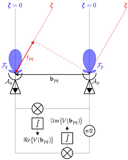
Figure 1.
Illustration of the principle of aperture synthesis radiometry. All the elementary antennas of an interferometric array, here reduced to two antennas and separated by a baseline , are pointing in the same direction, depicted here by the main beam of the elementary patterns and (in blue). The radio signal kept by each elementary antenna is coming from any direction of the surrounding space. Referring to the integral in (1), the contribution from direction (in red) depends on the delay between the time a wave train (dashed red) arrives on antenna and its arrival on antenna . For the contribution from the nadir looking direction (in blue), this delay is equal to zero. The two radio signals are transmitted to a complex correlation unit to be combined in-phase/in-quadrature and integrated in order to provide the real and imaginary parts of the complex visibility sample V for the baseline vector . To make the illustration simpler without losing anything of the interpretation of Equation (1), amplifiers, local oscillators, and band-pass filters are intentionally omitted (more details can be found in [6]).
The relationship between the complex visibilities and the brightness temperature of the scene under observation has been revisited in order to take into account the mutual coupling of close antennas [13]. Without polarimetric considerations [14], the complex visibility for a pair of elementary antennas and is given by:
where is the baseline vector associated with the two antennas and located in and in , the components , , and of the angular position variable are direction cosines in the reference frame of the array, and are the traditional spherical coordinates (the colatitude and the azimuth, respectively), and are the voltage patterns of the two antennas (for the readers not familiar with antennas patterns, the difference between amplitude, or voltage, patterns and power patterns can be found in the definition of radiation patterns in [15]) with equivalent solid angles and , as defined by Equations (2)–(24) in [16], is the brightness temperature distribution of the scene under observation, is the physical temperature of the receivers (assumed to be the same for all the receivers), is the fringe-washing function that accounts for spatial decorrelation effects, as defined by Equation (3) in [17], with the spatial delay and the central wavelength of observation.
After discretization of the double integral in modeling Equation (1) over an appropriate sampling grid in the direction cosines domain, the relationship between the complex visibilities V and the brightness temperature distribution of the scene under observation can be written in the linear algebraic form:
where is the linear modeling matrix of the instrument. The inverse problem aims at retrieving (the constant is canceled out from the visibilities with the aid of the response to a flat target [18], whatever the method used for the inversion [19]). As this inverse problem is ill-posed [20], it has to be regularized in order to provide a unique and stable solution for T. Among the regularization methods [21], the minimum-norm solution is widely used in imaging radiometry [22]:
This map is obtained through the computation of the Moore–Penrose [23,24] pseudo-inverse of :
In order to filter out the Gibbs effects [25] due to the sharp frequency cut-off associated with the limited extent of the experimental frequency coverage of the instrument, has to be damped by an appropriate windowing function: [26]. This map has to be compared to (which is the “ideal” temperature map to be reconstructed and apodized with the same window W) and not to T (which is not at the same spatial resolution).
3. Sky vs. Earth Observations with Antenna Arrays
Radio astronomers and the remote sensing community are both using aperture synthesis to obtain images of the sky or of Earth’s surface at radio frequencies from interferometric measurements provided by antenna arrays. However, although for historical reasons the latter have been inspired by the former, there are few differences that deserve attention. This is particularly true when focusing on the relation between the extent of the synthesized field of view and the spacing between the elementary antennas of the arrays. Indeed, regardless of the angular resolution, which depends on the longest separation between antenna pairs, the key parameter of an aperture synthesis interferometer in radio astronomy is the extent of the synthesized field of view, whereas in Earth remote sensing the key parameter is the shortest spacing between the antennas. Although it is well-known that both are closely related, it is explained hereafter why the remote sensing community deduces the extent of the synthesized field of view from the antenna spacing, and why the radio astronomers proceed in the opposite way.
3.1. The Radio Astronomy Point of View
In radio astronomy, the field of view (FOV) of an interferometer is determined by the size of the individual antennas and by the observing frequency (or wavelength) [6]. It is expressed in terms of the primary beam, which is nothing but the antenna response as a function of the angle away from the main axis. The full-width-at-half-maximum (FWHM) of the primary beam is usually taken as the diameter of the field of view synthesized by the interferometer; however, it is well-known that the sensitivity is not uniform over this field of view, which has a maximum at the center and tapers off towards the edges. The principle of aperture synthesis is to mix the signals from an array of antennas to obtain images having the same angular resolution as an instrument the size of the entire collection. The signals collected by the elementary antennas of the array are combined pairwise in a correlation unit to produce interferometric data known as complex visibilities. An image of the sky brightness distribution is reconstructed from these visibilities with the aid of the computer. These measurements have continuous coordinates because the elementary antennas of the arrays are non-regularly spaced and because they point outside the zenith direction as Earth rotates. As a consequence, for computational reasons, these complex visibilities first need to be resampled onto a regular grid before being inverted. This preliminary step is called “gridding” [27]. The relation between the sampling step d of that regular grid and the overall angular extent of the synthesized field of view is to be found in the Fourier theory:
where is the observing wavelength. For example, for every elementary 15 m antenna of the NOEMA millimeter interferometer [28], the primary beam is about at 100 GHz ( mm). As a consequence, here the sampling step d is about , that is to say, 12 m. As the antennas can move on rail tracks up to a maximum separation of 760 m in the E-W direction and 368 m in the N-S direction, the minimum number of pixels to satisfy the Shannon sampling theorem [29] is . With the most extended configuration of the array, the resolution is about . As the pixel size is , the synthesized beam is about five pixels wide. Finally, due to the diameter of the antenna dishes and to the observing frequency, it is important to keep in mind that with radio-astronomy interferometers, the overall extent of the synthesized field of view is much smaller than the sr space in front of the instrument. To fix the ideas concretely, with NOEMA, the solid angle is about 48 nsr.
3.2. The Remote Sensing Point of View
Unlike interferometers observing the sky in radio astronomy, which fall into the category of non-regular antenna arrays requiring a gridding preliminary step prior to the inversion of the visibilities, the antenna arrays observing Earth from a low-elevation orbit (LEO) belong, or will belong, for space accommodation reasons to the family of regular antenna arrays leading to a regular sampling of the experimental frequency coverage. As a consequence, in Earth remote sensing, the overall angular extent of the field of view of an interferometer is determined by the shortest spacing d between the antennas and by the observing wavelength :
When the instrument points into the nadir direction, as illustrated in Figure 1, Earth is a disk with a radius in the direction cosines domain of the reference frame attached to the antenna array, where is the radius of Earth and h is the elevation of the platform. To fix the ideas, from the elevation of SMOS, km, Earth is seen from an angle and it subtends a solid angle sr. Due to the Y-shaped geometry of the interferometric array and to the spacing between the antennas, with cm, the synthesized field of view of SMOS is a hexagon with outer radius [26] in the direction cosines domain of the same reference frame, that is to say, . Such a hexagonal field of view subtends a solid angle sr. This value is very far from those encountered in radio astronomy as it is an important fraction of the sr space in front of the instrument. With regards to the voltage patterns of the elementary antennas, it turns out that the averaged FWHM is about , which is comparable to the overall angular extent of the hexagonal field of view . Finally, with three arms as long as m, the best angular resolution of SMOS is about with a Blackman apodization window [30]. As the number of pixels sampling the hexagonal field of view is set to , the size of the hexagonal pixels is about in the boresight direction. As a consequence, the synthesized beam is more than three pixels wide.
4. Geometrical Considerations
For a regularly spaced antenna array leading to a Cartesian sampling of the Fourier space and therefore of the dual space of the brightness temperature distributions in the direction cosines domain, the synthesized field of view is a square of sides . As a consequence, it remains included in the sr space in front of the instrument as soon as . Likewise, for a regularly spaced antenna array leading to a hexagonal sampling, the synthesized field of view is now a hexagon of sides . As a consequence, it remains included in the same unit circle as soon as . These two situations are illustrated in Figure 2.
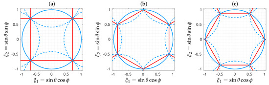
Figure 2.
Synthesized field of view (red) and limit of the sr space (blue) in front of antenna arrays leading to (a) a Cartesian geometry here with and to (b,c) a hexagonal geometry here with . The components , , and of the angular position variable are direction cosines in the reference frame of the arrays, and are the traditional polar coordinates (the colatitude and the azimuth, respectively). Shown with dashed blue lines are the sky aliases. Earth (and its aliases) is not shown as its location, and its extent in this direction cosines domain depends on the elevation and on the attitude of the platform.
As soon as becomes smaller than these two limits, the vertices of the synthesized fields of view go beyond the unit circle. The corresponding directions have neither a physical meaning nor a mathematical one, as they correspond to situations where would be larger than 1. Contrary to what one might quickly think, these directions are not in the sr space in the back of the antenna array. Indeed, these back directions fold on the front ones in the direction cosines domain according to the trigonometric identity and, of course, they satisfy the condition . As a consequence, they cannot be taken into account in the inversion process. However, there is no physical reason not to attempt to inverse the visibilities with the goal of retrieving the brightness temperature distributions only for those directions of the synthesized field of view included in the unit circle. Unfortunately, it will be shown in the next sections that this limited aperture synthesis operation is unstable in the presence of noise or errors. Shown in Figure 3 are the variations of this proportion of directions with the shortest spacing between the antennas. In every case, two regions are well-separated: in the first one this fraction is strictly equal to zero, whereas in the second one it is a growing function of the inverse of the shortest spacing. The frontier between these regions is between and with the Cartesian geometry, and it is between and with the hexagonal ones. In both cases, it is slightly below the theoretical values shown in Figure 2, as a consequence of the discrete sampling of the synthesized field of view, here with regularly spaced directions (or pixels) . As a very simple consequence of the fact that a hexagon has six vertices whereas a square has only four, the variations are more abrupt for the hexagonal geometries than for the Cartesian one.
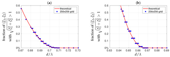
Figure 3.
Variations of the fraction of directions without physical or mathematical meaning with the shortest spacing d between the antennas of arrays leading to (a) a Cartesian geometry and to (b) a hexagonal geometry. Shown in red are the theoretical variations and with blue bullets the values calculated for sampling grids with directions (or pixels) in the synthesized field of view. In every case, two regions are well-separated: in the first one this fraction is strictly equal to zero, whereas in the second one it is a growing function of the inverse of the shortest spacing. The frontier between these regions is estimated between and in (a) and between and in (b).
5. Numerical Simulations
In the absence of any other additional information, it is not possible to quantify the impact of Figure 3 on the stability of an inversion process in such situations and on the quality of the final brightness temperature maps thus obtained. There is no other way than to conduct a parametric study with the aid of numerical simulations for an antenna array where the shortest spacing plays the central role.
5.1. Antenna Array
Numerical simulations have been conducted within the frame of the SMOS-HR project [11] for a cross-shaped array equipped with 167 antennas, as illustrated in Figure 4. This number includes two additional antennas in order to meet the redundancy requirement for being calibrated with the aid of the redundant spacing calibration method [31]. All the antennas are assumed to provide a measure of the average brightness temperature of the scene (contrary to what is done for SMOS where it relies only on few measurements provided by three reference radiometers [32]). The spacing between the antennas along the arms is set to , and one arm is judiciously translated with respect to the others so that the shortest spacing between the closest antennas is reduced down to d. This design, which increases the angular extent of the synthesized field of view, and therefore reduces the aliasing, has been patented [33]. If at ground level the useful swath across the track of the satellite depends on the elevation h of the platform above Earth’s surface and on its orientation with respect to the nadir looking direction, the main driver turns out to be the ratio , as introduced in Section 3. To complete the modeling of the instrument, here h has been fixed to 685 km and to for practical reasons. However, this parametric study is not sensitive to variations of h or .
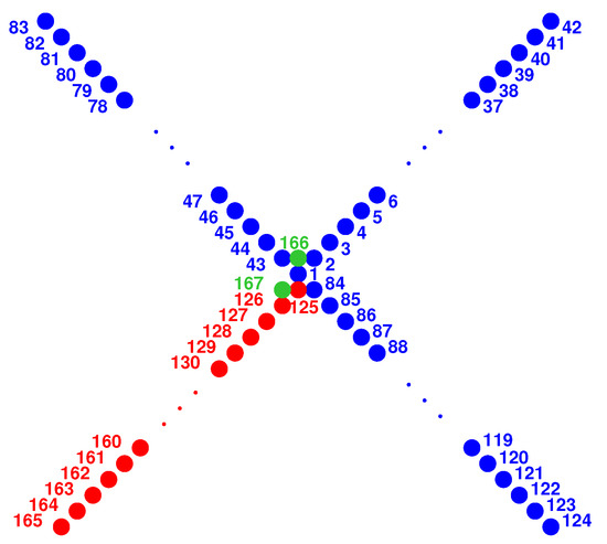
Figure 4.
A cross-shaped array populated with 167 antennas. The red arm is translated with respect to the three others in blue, and the green antennas are added for calibration purposes. The spacing between the closest antennas, as illustrated, for example, by antennas #125 and #1, or by antennas #166 and #2, is set to d. As a consequence of the geometry, the spacing between the antennas along the arms is equal to .
5.2. Modeling Matrix
Referring back to (2), for an array of elementary antennas, the number of baselines, and therefore the number of complex visibilities, is . Assuming that each elementary antenna also provides a measure of the average brightness temperature of the scene, the total number of real valued measurements is . As a consequence, the dimensions of the modeling matrix are therefore , where is the number of pixels of a sampling grid in the synthesized field of view. To fix the ideas, for the cross-shaped array shown in Figure 4, these dimensions are . As a consequence of the geometry of the array, out of these measurements, only are non-redundant: they correspond to the Fourier frequencies of the so-called experimental frequency coverage.
The singular values decomposition [34] of the rectangular matrix is a factorization that involves the singular values ordered in descending order and two and unitary matrices and so that the factorization reads
where , resp. , is the ℓth column of , resp. . Shown in Figure 5 are the distributions of the singular values of the modeling matrix of the antenna array of Figure 4 when the shortest spacing d between the elementary antennas is set to or to , two values on each side of the frontier . In every case, two groups of singular values separated by a well-determined gap are observed: the first group is composed of the largest singular values, the second one of the remaining smallest ones. In numerical linear algebra, the singular value decomposition can be used to determine the effective rank of a matrix [35], as rounding errors may lead to small but non-zero singular values with a rank deficient matrix [36]. From the numerical point of view, singular values beyond a given threshold are assumed to be numerically equivalent to zero. This threshold is often set to the so-called -machine, which is equal to in MATLAB [37]. The truncated singular value decomposition [38] is no longer an exact decomposition of the original matrix , but rather provides the optimal low-rank matrix approximating it:
where only the first singular values are taken into account, the other ones being discarded because they are equal to zero from the numerical point of view, as illustrated in Figure 5. As a consequence of this rank deficiency [36] of , the pseudo inverse of the regularized matrix is given by the decomposition:
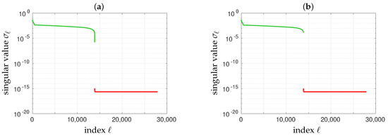
Figure 5.
Distributions of the singular values of the modeling matrix of the cross-shaped array shown in Figure 4 for two values of the shortest spacing: (a) and (b) . In every case, two groups of singular values separated by a well-determined gap are observed: the first group (green) is composed of the 13861 largest singular values, the second one (red) of the remaining smallest ones that could be considered as being equal to zero.
This decomposition does not give rise to any problem because the smallest singular values (and in particular those equal to zero) no longer play any role in the inversion. In such a situation, the propagation of random errors from the complex visibilities V to the retrieved brightness temperature distribution
is governed by the so-called condition number [39] of the regularized modeling matrix , which is defined by the ratio:
By definition, as the singular values are ordered in descending order, this ratio is larger than 1. However, it should be kept in mind that this value is an upper bound for this propagation. For example, referring back to Figure 5, with , whereas with . Shown in Figure 6 are the variations of with the shortest spacing d. As noted in Figure 3a, here again two regions are well-separated: in the first one the value of is almost constant, whereas in the second one it is a growing function of the inverse of the shortest spacing. The frontier between these regions is estimated anew between and .
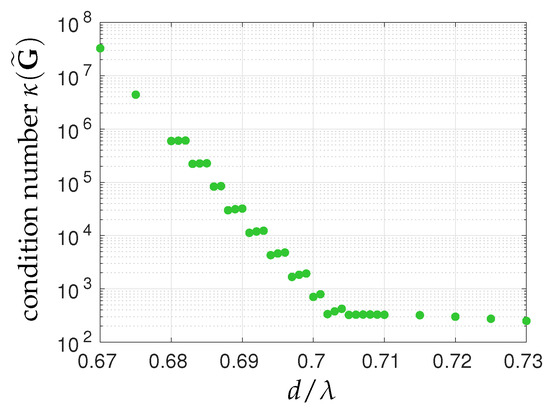
Figure 6.
Variations of the condition number of the regularized modeling matrix of the cross-shaped array shown in Figure 4 with the shortest spacing d between the 167 elementary antennas. This figure has to be compared to Figure 3a as here again two regions are well-separated: in the first one is almost constant, whereas in the second one it is a growing function of the inverse of the shortest spacing. The frontier between these regions is estimated between and .
5.3. Noiseless Inversions
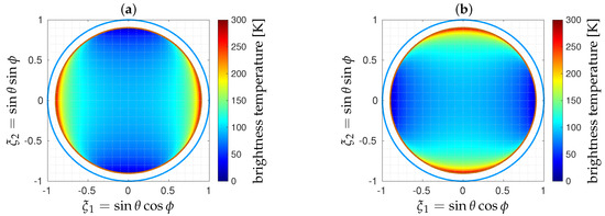
Complex visibilities V have been simulated according to (1) for a typical scene T over the ocean [40], as illustrated in Figure 7. They have been inverted according to (9), and the retrieved brightness temperature distributions have been apodized with a Blackman apodization window for comparison with , which is at the same angular resolution and apodized with the same Blackman window.
Shown in Figure 8 are the error maps when the shortest spacing d is set to or to . As expected, the reconstruction error is almost equal to 0 in both cases, whatever the polarization. In this ideal noiseless situation, the retrieved brightness temperature maps are not sensitive to the spacing between the antennas.
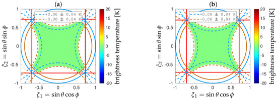
Figure 8.
Error maps obtained in X polarization with the cross-shaped array shown in Figure 4 for two values of the shortest spacing: (a) and (b) (similar results are obtained in Y polarization). In both cases, complex visibilities V are free from any additional random noise . Referring back to Figure 2, Earth aliases are shown with dashed maroon lines. Bias and standard deviation are given in Earth alias-free FOV (dashed maroon line) and in the sky alias-free FOV (dashed blue line).
5.4. Noisy Inversions
Previous complex visibilities V have been blurred with an additive Gaussian noise with standard deviation K. Shown in Figure 9 are the error maps for the same random distribution when the shortest spacing d is set to or to . As expected, the reconstruction error is no longer equal to 0 in both cases: it is almost randomly distributed in the synthesized FOV, with values increasing from the boresight direction with the colatitude angle . However, when , a cross-shaped phantom is obviously superimposed on this random distribution.
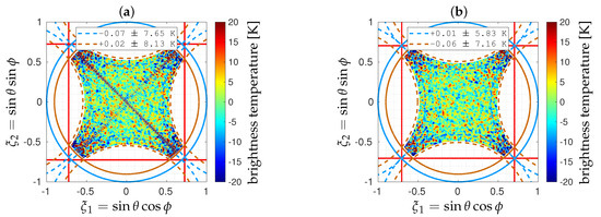
Figure 9.
Error maps obtained in X polarization with the cross-shaped array shown in Figure 4 for two values of the shortest spacing: (a) and (b) (similar results are obtained in Y polarization). In both cases, complex visibilities V have been blurred by an additive Gaussian noise with standard deviation set to K.
Average maps and standard deviation maps of 1000 error maps obtained for different random trials of with the same standard deviation K are shown in Figure 10 and Figure 11 for the same values of the shortest spacing. When the spacing d is equal to , the average error is almost equal to zero, except at high colatitude angles in the four corners of the FOV, close to those directions beyond the unit circle. With regards to the radiometric sensitivity [41], the minimum value of the standard deviation map is obtained at boresight. Away from that direction, errors are growing like the inverse of the average antenna radiation pattern times the factor , as expected. The same behavior is observed for , except the superimposition of that cross-shaped phantom in the average map as well as in the standard deviation one. Of course, the presence of this cross-shaped phantom is detrimental to any further use of such retrieved maps. The origin of this reconstruction artifact is analyzed hereafter, then a solution is proposed for removing it without altering the performance of the instrument.
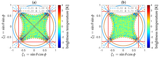
Figure 10.
Average maps of 1000 error maps obtained in X polarization with the cross-shaped array shown in Figure 4 for two values of the shortest spacing: (a) and (b) (similar results are obtained in Y polarization). In every case, complex visibilities V have been blurred by an additive Gaussian noise with standard deviation set to K.
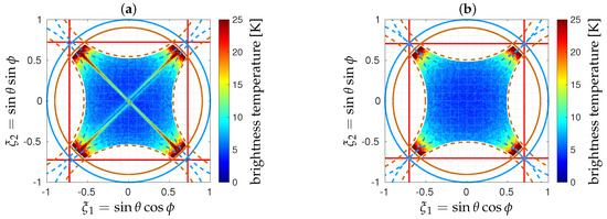
Figure 11.
Standard deviation maps of 1000 error maps obtained in X polarization with the cross-shaped array shown in Figure 4 for two values of the shortest spacing: (a) and (b) (similar results are obtained in Y polarization). In every case, complex visibilities V have been blurred by an additive Gaussian noise with standard deviation set to K.
Because the two matrices and are unitary, the corresponding singular vectors and form an orthonormal basis of the underlying real-valued spaces and . As a consequence, the retrieved brightness temperature distribution can be decomposed onto the space spanned by the according to the expansion [42]
Of course, the sum is restricted to the singular vectors corresponding to the singular values kept in the inversion of , and the inner product is simply the sum of the products between every component of and those of on the grid sampling the FOV. In numerical linear algebra, the error analysis is often initiated by computing the separation angle between the numerical solution of a linear system and every singular vector of the corresponding matrix and especially with those associated to the smallest singular values because their role during the inversion has to be carefully taken into account. The separation angle between the solution and the ℓth singular vector of the modeling matrix is derived from the well-known definition of the inner product [42]:
Referring back to (11), the farther to , the more important the contribution of to the retrieved brightness temperature map . Shown in Figure 12 and Figure 13 are the variations of with the singular values of Figure 5 for the retrieved brightness temperature maps of Figure 8 and Figure 9. In the absence of any additive Gaussian noise , whatever the shortest spacing, or , all the separation angles are confined to the interval except . As a consequence, apart from , which has the largest contribution to , there is no singular vector with a greater contribution than another. This is not surprising, as contributes to the average value of and is associated with the largest singular value . As soon as the complex visibilities V are blurred with an additive Gaussian noise , the distribution of the separation angles varies from one shortest spacing to another. When , the situation in Figure 13b is very similar to that in Figure 12b in the absence of noise: this is the reason why no cross-shaped phantom is observed in the retrieved brightness temperature map of Figure 9b, the average map Figure 10b, and in the standard deviation map of Figure 11b. On the contrary, when , there are singular vectors that contribute more to than as illustrated by their separation angles, which are farther from than is. Moreover, these excited singular vectors correspond to the smallest singular values kept in the inversion of . Referring back to (8) and to the role played by these singular values, it would not be surprising to see these singular vectors in the error map of Figure 9a. This is exactly what is proven in Figure 14 with the singular vectors of corresponding to the three smallest singular values , , and . In addition to being associated with the smallest singular values, these three singular vectors are particularly excited in the error map of Figure 9a as the separation angles are, respectively, , , and . Indeed, referring back to (12) and (11), the contribution of the corresponding three singular vectors to is about two thirds. More precisely, it is larger than for and for as well and about for . When comparing these singular vectors to the error map of Figure 9a, there is no doubt that the cross-shaped phantom seen in this map is a linear combination of them. The origin of this artifact is therefore coming from the modeling matrix itself and from the way it propagates the additive Gaussian noise from the complex visibilities V to the retrieved brightness temperature map , and therefore to the apodized one , during the inversion process. As a consequence, the cure has to be found in the regularization of .
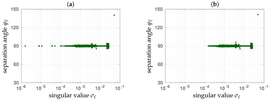
Figure 12.
Separation angles between the singular vectors of and the brightness temperature maps corresponding to the apodized maps of Figure 8 retrieved without radiometric noise for two values of the shortest spacing of the cross-shaped array shown in Figure 4: (a) and (b) . Only the first largest singular values shown in green in Figure 5 are reported here inasmuch as the other ones are discarded prior to the inversion of , the corresponding singular vectors do not contribute to .
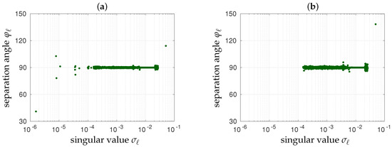
Figure 13.
Separation angles between the singular vectors of and the brightness temperature maps corresponding to the apodized maps of Figure 9 retrieved when complex visibilities V are blurred by an additive Gaussian noise with standard deviation set to K for two values of the shortest spacing of the cross-shaped array shown in Figure 4: (a) and (b) . Only the first largest singular values shown in green in Figure 5 are reported here inasmuch as the other ones are discarded prior to the inversion of , the corresponding singular vectors do not contribute to .
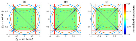
Figure 14.
Singular vectors of corresponding to the smallest singular values when the shortest spacing of the cross-shaped array shown in Figure 4 is set to . Only the last three singular vectors are shown here for (a) with , (b) with , and (c) with . Components of are normalized according to property because matrix is unitary.
Figure 13a strongly suggests revisiting the truncated singular value decomposition of when and to discard those small singular values and their singular vectors with a separation angle far from , so that the regularized modeling matrix now reduces to:
where is the number of additional singular values that will discarded prior to the inversion. As a consequence, the reconstruction operator is no longer but
and the retrieved brightness temperature distribution is now
Likewise, the condition number of the regularized modeling matrix is no longer but
If the number of singular values taken into account in the inversion of is not subjected to discussion because the other ones are equal to zero from the numerical point of view, as illustrated in Figure 5, the choice of a value for n is not obvious. When comparing Figure 12 and Figure 13 while keeping an eye to the singular vectors such as those shown in Figure 14, it turns out that is an appropriate value. As a consequence, the previous visibilities V have been inverted according to (15), with only singular values kept in the pseudo inverse of , which has a condition number close to 320, a value comparable to that of with . Shown in Figure 15 are the error maps obtained with and without a random Gaussian noise with standard deviation K. In contrast to Figure 9a, the propagation of during the inversion no longer results in the presence of an undesirable phantom, as expected with the filtering out of the singular vectors corresponding to the n smallest singular values. In the absence of noise, this severe truncation does not introduce any additional error in the retrieved brightness temperature map, as illustrated by the comparison with Figure 8a. Average maps and standard deviation maps of 1000 error maps obtained for different random trials of with the same standard deviation K are shown in Figure 16. Here again, unlike Figure 10a and Figure 11a, the cross-shaped phantom no longer disturbs these brightness temperature distributions. Due to this additional truncation of , the brightness temperature maps retrieved with for are almost identical to those retrieved with for , as illustrated by the comparison of Figure 15 and Figure 16 with Figure 8b, Figure 9b, Figure 10b, and Figure 11b. Referring back to the radiometric sensitivity [41], from a quantitative point of view, the minimum value at boresight is about K in the standard deviation map shown in Figure 11b with and about K in the standard deviation map shown in Figure 16b with . With regard to this latter situation, this estimation is about K in the standard deviation map shown in Figure 11a, as a consequence of the presence of the cross-shaped phantom. According to Equation (1) in [43], the radiometric sensitivity should be equal to K with and to K with . This additional truncation of therefore has no impact on the radiometric sensitivity, as the estimation is still following the theoretical value with the same uncertainty.
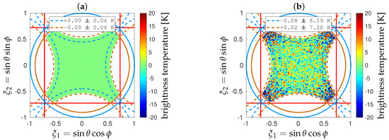
Figure 15.
Error maps obtained in X polarization with the cross-shaped array shown in Figure 4 with the shortest spacing d set to when (a) complex visibilities V are free from any additional random noise and when (b) complex visibilities V are blurred by an additive Gaussian noise with standard deviation set to K (similar results are obtained in Y polarization). In both cases, the singular vectors of corresponding to the 16 smallest singular values have been discarded prior to the inversion. These maps have to be compared to those in Figure 8a and Figure 9a where these singular vectors were taken into account in the computation of .
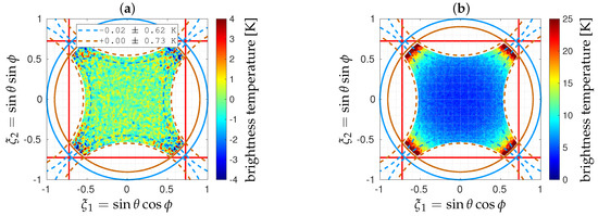
Figure 16.
Average map (a) and standard deviation map (b) of 1000 error maps obtained in X polarization with the cross-shaped array shown in Figure 4 with the shortest spacing d set to (similar results are obtained in Y polarization). In every case, complex visibilities V have been blurred by an additive Gaussian noise with standard deviation set to K and the singular vectors of corresponding to the 16 smallest singular values have been discarded prior to the inversion. These maps have to be compared to those in Figure 10a and Figure 11a where these singular vectors were taken into account in the computation of .
Finally, the impact of this supplementary truncation of onto the angular resolution also has to be addressed. It turns out that the synthetic response of the cross-shaped array of Figure 4 with is almost identical to that with as a consequence of the small number of additional singular vectors discarded prior to the inversion: although these singular vectors might be associated with high-resolution features, the spectral content in the remaining singular vectors is almost identical to that in the ones. In both cases, the angular resolution is about without an apodization window and about with a Blackman apodization window, as illustrated in Figure 17.
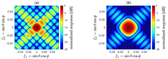
Figure 17.
Closed views of the normalized synthetic responses of the cross-shaped array shown in Figure 4 when the shortest spacing d is set to . The FWHM value of the main beam, here illustrated by the black circles, is about (a) without an apodization window and about (b) with a Blackman apodization window. Here, the reconstruction operator is ; identical responses are obtained with when additional singular values are discarded prior to the inversion.
6. Discussion and Remarks
The same cross-shaped phantom is observed for any shortest spacing and for the same reasons it is caused by these singular vectors of corresponding to the smallest singular values , which are responsible for an unacceptable propagation of noise from complex visibilities to retrieved brightness temperature maps. In any case, it can be filtered out with the same truncated singular value decomposition of where the last n singular vectors that exhibit partial or complete features of this cross-shaped phantom are discarded prior to inversion according to (14), keeping the propagation of noise at an acceptable level. Whatever the shortest spacing d, the appropriate value for n seems to be linearly correlated with the number of directions of the synthesized field of view that are not taken into account in the inversion, as illustrated in Figure 3a. More precisely, it turns out that the correlation coefficient between n and this number of rejected directions is better than , and the slope of the linear regression between them is very close to 4. This is not surprising, as 4 is the number of vertices of the square-shaped synthesized field of view, which suggests that the key parameter is not the total number of directions but the number of directions per vertex. Each direction in a given vertex is intimately related to another one in the three other vertices, and they are all together responsible for the same suspicious singular vector. Finally, referring back to Figure 2b,c and Figure 3b, a similar phantom is observed with a hexagonal geometry for any shortest spacing : this is the case for the SMOS-HEX project [43].
The singular value decomposition of the modeling matrix strongly depends on the voltage pattern of each elementary antenna of the interferometric array. This is very well illustrated by Figure 1 in [44] with the disparity among the 69 voltage patterns of SMOS that have been measured in an anechoic chamber prior to the launch [45]. As a consequence, the n singular vectors to be filtered out in the retrieved brightness temperature distribution (15) may vary with these voltage patterns. This is why these patterns have to be measured in their environment [46], as accurately as possible, in order to precisely compute the modeling matrix and its singular value decomposition so that the singular vectors that may propagate noise inappropriately during the inversion process can be clearly identified and filtered out, if necessary.
Finally, depending on the extent of the frequency bandwidth of observation, a wide band is often divided into smaller sub-bands for many reasons: reducing the fringe washing effects caused by large spatial decorrelation [47], filtering out the radio frequency interference [48], etc. As a consequence, the fraction will vary linearly with the frequency from one channel to the other. The situation where few sub-bands (those for the lowest frequencies of the wide band) might suffer from that issue and few others (those for the highest frequencies) might not cannot be excluded. On the contrary, it has to be taken into account when selecting the shortest spacing d between the elementary antennas of the array, because the approach for inverting multi-channel visibilities may vary from one sub-band to the other. As an illustrative example, consider the L-band radiometry case with observations in a bandwidth of 24 MHz centered on MHz. With a short spacing mm, the fraction is equal to in the very center of the bandwidth, but it varies from for the lowest frequency of the bandwidth to for the highest one. Referring back to Figure 6, the corresponding condition number varies from 4300 to 320. As sub-band processing raises many other issues (sampling grids, useful swath, angular resolution, radiometric sensitivity, etc., that may vary from one sub-band to another) in addition to this conditioning problem, it deserves a dedicated study that will be addressed in a forthcoming paper.
7. Conclusions
The truncated singular value decomposition has always been used as a regularization tool in order to obtain a unique solution (the minimum norm one) to a rank-deficient inverse problem. This is exactly what has been done in imaging radiometry by aperture synthesis for a long time. The number of singular values kept in the inversion is here equal to the number of Fourier frequencies in the experimental frequency coverage of the interferometric array of antennas. This comfortable situation has never been questioned unless recent studies have evidenced a potential issue when the shortest spacing between the antennas of an interferometric array is chosen is such a way that some viewing directions of the synthesized field cannot be taken into account in the inversion process because they have neither a physical meaning nor a mathematical one.
This issue has been illustrated with the aid of numerical simulations conducted within the frame of the SMOS-HR project. However, it is also explained why this problem will affect any interferometric array as soon as the shortest spacing between the elementary antennas becomes smaller than a geometrical limit, which only depends on the geometry of the underlying sampling grids. It has been shown that, in such a situation, the inversion of the complex visibilities becomes unstable in the presence of noise, and this instability is characterized by the undesirable presence of a phantom in the retrieved brightness temperature maps. The origin of this phantom has been explained, and a solution to cure the interferometric array from that issue has been proposed and assessed.
From the linear algebra point of view, this study has illustrated that the truncated singular value decomposition can also be used as a conditioning tool in order for the unique solution of a rank-deficient inverse problem to be a stable one with regard to the propagation of noise or errors during the inversion process. Provided that the number of additional singular values to discard prior to the inversion is acceptable, the radiometric sensitivity and the angular resolution do not suffer from this supplementary truncation. The smaller the shortest spacing below that geometrical limit, the stronger the propagation of noise and the larger the number of additional singular values to be discarded for reducing the presence of that phantom in the retrieved brightness temperature maps.
Author Contributions
Conceptualization, E.A. and L.Y.; methodology, E.A. and L.Y.; software, E.A.; validation, E.A. and L.Y.; formal analysis, E.A. and L.Y.; investigation, E.A. and L.Y.; resources, E.A.; data curation, E.A.; writing—original draft preparation, E.A.; writing—review and editing, E.A. and L.Y.; visualization, E.A.; supervision, E.A.; project administration, E.A. and L.Y. All authors have read and agreed to the published version of the manuscript.
Funding
This work was supported by the French National Research Council (CNRS) within the frame of the SMOS-HR (Soil Moisture and Ocean Salinity at High-Resolution) project led by the French Space Agency (CNES) currently undergoing phase A studies.
Data Availability Statement
Data are available upon request by email to the corresponding author.
Acknowledgments
The authors are very grateful to Yann Kerr (CESBIO) and Thierry Amiot (CNES) for their constant support and encouragement during this work. Data processing support was provided by CESBIO and CNES. The authors are indebted to the associate editor and to the four anonymous reviewers for their helpful reviews which greatly improved the manuscript.
Conflicts of Interest
The authors declare no conflict of interest.
References
- Barré, H.; Duesmann, B.; Kerr, Y.H. SMOS: The Mission and the System. IEEE Trans. Geosci. Remote Sens. 2008, 46, 587–593. [Google Scholar] [CrossRef]
- McMullan, K.D.; Brown, M.A.; Martín-Neira, M.; Rits, W.; Ekholm, S.; Lemanczyk, J. SMOS: The Payload. IEEE Trans. Geosci. Remote Sens. 2008, 46, 594–605. [Google Scholar] [CrossRef]
- Kerr, Y.H.; Waldteufel, P.; Richaume, P.; Wigneron, J.-P.; Ferrazzoli, P.; Mahmoodi, A.; Al Bitar, A.; Cabot, F.; Gruhier, C.; Enache Juglea, S.; et al. The SMOS Soil Moisture Retrieval Algorithm. IEEE Trans. Geosci. Remote Sens. 2012, 50, 1384–1403. [Google Scholar] [CrossRef]
- Zine, S.; Boutin, J.; Font, J.; Reul, N.; Waldteufel, P.; Gabarró, C.; Tenerelli, J.; Petitcolin, F.; Vergely, J.-L.; Talone, M.; et al. Overview of the SMOS Sea Surface Salinity Prototype Processor. IEEE Trans. Geosci. Remote Sens. 2008, 46, 621–645. [Google Scholar] [CrossRef]
- de Rosnay, P.; Rodriguez-Fernandez, N.; Munoz-Sabater, J.; Albergel, C.; Fairbairn, D.; Lawrence, H.; English, S.; Drusch, M.; Kerr, Y.H. SMOS Data Assimilation for Numerical Weather Prediction. In Proceedings of the International Geoscience and Remote Sensing Symposium (IGARSS 2018), Valencia, Spain, 22–27 July 2018. [Google Scholar]
- Thompson, A.R.; Moran, J.W.; Swenson, G.W. Interferometry and Synthesis in Radio Astronomy, 3rd ed.; Springer International Publishing: Cham, Switzerland, 2017. [Google Scholar]
- Thompson, A.R.; Clark, B.G.; Wade, C.M.; Napier, P.J. The Very Large Array. Astrophys. J. Suppl. Ser. 1980, 44, 151–167. [Google Scholar] [CrossRef]
- Padin, S.; Shepherd, M.C.; Cartwright, J.K.; Keeney, R.G.; Mason, B.S.; Pearson, T.J.; Readhead, A.C.S.; Schaal, W.A.; Sievers, J.; Udomprasert, P.S.; et al. The Cosmic Background Imager. Publ. Astron. Soc. Pac. 2002, 114, 83–97. [Google Scholar] [CrossRef]
- Anterrieu, É.; Rodriguez-Fernandez, N.J.; Rougé, B.; Cabot, F.; Richaume, P.; Khazâal, A.; Kerr, Y.H.; Morel, J.-M.; Colom, M.; Costeraste, J.; et al. Preliminary System Studies on a High-Resolution SMOS Follow-On: SMOS-HR. In Proceedings of the International Geoscience And Remote Sensing Symposium (IGARSS 2019), Yokohama, Japan, 28 July–2 August 2019. [Google Scholar]
- Jansen, S.; Pieters, M. The 7 Principles of Complete Co-Creation, 1st ed.; BIS Publishers: Amsterdam, The Netherlands, 2018. [Google Scholar]
- Rodriguez-Fernandez, N.J.; Anterrieu, É.; Cabot, F.; Boutin, J.; Picard, G.; Pellarin, T.; Merlin, O.; Vialard, J.; Vivier, F.; Costeraste, J.; et al. A New L-Band Passive Radiometer for Earth Observation: SMOS-High Resolution (SMOS-HR). In Proceedings of the International Geoscience And Remote Sensing Symposium (IGARSS 2020), Virtual Symposium, 26 September–2 October 2020; 2020. [Google Scholar]
- Anterrieu, É.; Khazâal, A. Brightness Temperature Maps Reconstruction from Dual-Polarimetric Visibilities in Synthetic Aperture Imaging Radiometry. IEEE Trans. Geosci. Remote Sens. 2008, 46, 606–612. [Google Scholar] [CrossRef]
- Corbella, I.; Duffo, N.; Vall-llossera, M.; Camps, A.; Torres, A. The Visibility Function in Interferometric Aperture Synthesis Radiometry. IEEE Trans. Geosci. Remote Sens. 2004, 42, 1677–1682. [Google Scholar] [CrossRef]
- Martín-Neira, M.; Ribó, S.; Martín-Polegre, A.J. Polarimetric Mode of MIRAS. IEEE Trans. Geosci. Remote Sens. 2002, 40, 1755–1768. [Google Scholar] [CrossRef]
- Roederer, A.; Antennas Committee. IEEE Std 145-2013: IEEE Standard for Definitions of Terms for Antennas; IEEE Publishing: New York, NY, USA, 2014; pp. 1–50. [Google Scholar]
- Balanis, C.A. Antenna Theory: Analysis and Design, 3rd ed.; John Wiley & Sons: Hoboken, NJ, USA, 2005. [Google Scholar]
- Kainulainen, J.; Rautiainen, K.; Hallikainen, M. Experimental Verification of Fringe-washing Calibration Techniques in Large Aperture Synthesis Radiometers. In Proceedings of the 9th Specialist Meeting on Microwave Radiometry and Remote Sensing Applications (μRad-2006), Juan, PR, USA, 28 February–3 March 2006. [Google Scholar]
- Martín-Neira, M.; Suess, M.; Kainulainen, J.; Martin-Porqueras, F. The Flat Target Transformation. IEEE Trans. Geosci. Remote Sens. 2008, 46, 613–620. [Google Scholar] [CrossRef]
- Corbella, I.; Torres, F.; Camps, A.; Duffo, N.; Vall-llossera, M. Brightness-Temperature Retrieval Methods in Synthetic Aperture Radiometers. IEEE Trans. Geosci. Remote Sens. 2009, 47, 285–294. [Google Scholar] [CrossRef]
- Hadamard, J. Sur les problèmes aux dérivés partielles et leur signification physique. Princet. Univ. Bull. 1902, 13, 49–52. [Google Scholar]
- Picard, B.; Anterrieu, É. Comparison of Regularized Inversion Methods in Synthetic Aperture Imaging Radiometry. IEEE Trans. Geosci. Remote Sens. 2005, 43, 218–224. [Google Scholar] [CrossRef]
- Goodberlet, M.A. Improved Image Reconstruction Techniques for Synthetic Aperture Radiometers. IEEE Trans. Geosci. Remote Sens. 2000, 38, 1362–1366. [Google Scholar] [CrossRef]
- Moore, E.H. On the Reciprocal of the General Algebraic Matrix. Bull. Am. Math. Soc. 1920, 26, 394–395. [Google Scholar]
- Penrose, R. A Generalized Inverse for Matrices. Math. Proc. Camb. Philos. Soc. 1955, 51, 406–413. [Google Scholar] [CrossRef]
- Hewitt, E.; Hewitt, R.E. The Gibbs-Wilbraham Phenomenon: An Episode in Fourier Analysis. Arch. Hist. Exact Sci. 1979, 21, 129–160. [Google Scholar] [CrossRef]
- Anterrieu, É.; Waldteufel, P.; Lannes, A. Apodization Functions for 2D Hexagonally Sampled Synthetic Aperture Imaging Radiometers. IEEE Trans. Geosci. Remote Sens. 2002, 40, 2531–2542. [Google Scholar] [CrossRef]
- Brouw, W.N. Aperture Synthesis. Methods Comput. Phys. 1975, 14, 131–175. [Google Scholar]
- Omont, A.; Pety, J.; Guelin, M. NOEMA-Une fenêtre sur les mondes en formation. L’Astronomie 2017, 131, 12–21. [Google Scholar]
- Shannon, C.E. Communication in the Presence of Noise. Proc. IRE 1949, 37, 10–21. [Google Scholar] [CrossRef]
- Kerr, Y.H.; Font, J.; Waldteufel, P.; Camps, A.; Bara, J.; Corbella, I.; Torres, F.; Duffo, N.; Vall-llossera, M.; Caudal, G. New Radiometers: SMOS-a Dual Pol L-band 2D Aperture Synthesis Radiometer. In Proceedings of the 2000 IEEE Aerospace Conference, Big Sky, MT, USA, 25 March 2000. [Google Scholar]
- Arnot, N.R.; Atherton, P.D.; Greeaway, A.H.; Noordam, J.E. Phase Closure in Optical Astronomy. Trait Signal 1985, 2, 129–136. [Google Scholar]
- Colliander, A.; Tauriainen, S.; Auer, T.I.; Kainulainen, J.; Uusitalo, J.; Toikka, M.; Hallikainen, M.T. MIRAS Reference Radiometer: A Fully Polarimetric Noise Injection Radiometer. IEEE Trans. Geosci. Remote Sens. 2005, 43, 1135–1143. [Google Scholar] [CrossRef]
- Kerr, Y.H.; Khazâal, A.; Cabot, F.; Rougé, B.; Lesthievent, G.; Monjid, Y.; Suere, C.; Rodriguez-Fernandez, N.; Anterrieu, É.; Richaume, P. Système d’Imagerie Radiométrique; Publication Number 3 071 068, Registration Number 17 58533; Institut National de la Propriété Industrielle: Paris, France, 2017. [Google Scholar]
- Golub, G.; Kahan, W. Calculating the Singular Values and Pseudo-Inverse of a Matrix. J. Soc. Ind. Appl. Math. Ser. B 1965, 2, 205–224. [Google Scholar] [CrossRef]
- Roy, O.; Vetterli, M. The Effective Rank: A Measure of Effective Dimensionality. In Proceedings of the 15th European Signal Processing Conference, Poznan, Poland, 3–7 September 2007; pp. 606–610. [Google Scholar]
- Hansen, P.C. Rank-Deficient and Discrete Ill-Posed Problems, 1st ed.; Society for Industrial & Applied Mathematics: Philadelphia, PA, USA, 1998. [Google Scholar]
- Matlab Function Reference. Available online: https://fr.mathworks.com/help/matlab/ref/eps.html (accessed on 1 January 2023).
- Hansen, P.C. The Truncated SVD as a Method for Regularization. BIT Numer. Math. 1987, 27, 534–553. [Google Scholar] [CrossRef]
- Cline, A.K.; Moler, C.B.; Stewart, G.W.; Wilkinson, J.H. An Estimate for the Condition Number of a Matrix. SIAM J. Numer. Anal. 1979, 16, 368–375. [Google Scholar] [CrossRef]
- Klein, L.; Swift, C. An Improved Model for the Dielectric Constant of Sea Water at Microwave Frequencies. IEEE J. Ocean. Eng. 1977, 2, 104–111. [Google Scholar] [CrossRef]
- Camps, A.; Corbella, I.; Barà, J.; Torres, F. Radiometric Sensitivity Computation in Aperture Synthesis Interferometric Radiometry. IEEE Trans. Geosci. Remote Sens. 1998, 36, 680–685. [Google Scholar] [CrossRef]
- Spiegel, M.; Lipschutz, S.; Spellman, D. Vector Analysis, 2nd ed.; McGraw-Hill Education: New York, NY, USA, 2009. [Google Scholar]
- Zurita, A.M.; Corbella, I.; Martín-Neira, M.; Plaza, M.A.; Torres, F.; Benito, F.J. Towards a SMOS Operational Mission: SMOSOps-Hexagonal. IEEE J. Sel. Top. Appl. Earth Obs. Remote Sens. 2013, 6, 1769–1780. [Google Scholar] [CrossRef]
- Anterrieu, É.; Palacin, B.; Costes, L. A New Metric for Estimating the Disparity of Antenna Patterns in Synthetic Aperture Imaging Radiometry. IEEE J. Sel. Top. Appl. Earth Obs. Remote Sens. 2020, 13, 5800–5906. [Google Scholar] [CrossRef]
- Pivnenko, S.; Nielsen, J.M.; Cappellin, C.; Lemanczyk, G.; Breinbjerg, O. High-Accuracy Calibration of the SMOS Radiometer Antenna Patterns at the DTU-ESA Spherical Near-Field Antenna Test Facility. In Proceedings of the International Geoscience and Remote Sensing Symposium (IGARSS 2007), Barcelona, Spain, 1–7 July 2007. [Google Scholar]
- Camps, A.; Skou, S.; Torres, F.; Corbella, I.; Duffo, N.; Vall-llossera, M. Considerations About Antenna Pattern Measurements of 2-D Aperture Synthesis Radiometers. IEEE Geosci. Remote Sens. Lett. 2006, 3, 259–261. [Google Scholar] [CrossRef]
- Fischman, M.A.; England, A.W. A Technique for Reducing Fringe Washing Effects in L-band Aperture Synthesis Radiometry. In Proceedings of the International Geoscience And Remote Sensing Symposium (IGARSS 2000), Honolulu, HI, USA, 24–28 July 2000. [Google Scholar]
- Subbaram, H.; Abend, K. Interference Suppression via Orthogonal Projections: A Performance Analysis. IEEE Trans. Antennas Propag. 1993, 41, 1187–1194. [Google Scholar] [CrossRef]


Disclaimer/Publisher’s Note: The statements, opinions and data contained in all publications are solely those of the individual author(s) and contributor(s) and not of MDPI and/or the editor(s). MDPI and/or the editor(s) disclaim responsibility for any injury to people or property resulting from any ideas, methods, instructions or products referred to in the content. |
© 2023 by the authors. Licensee MDPI, Basel, Switzerland. This article is an open access article distributed under the terms and conditions of the Creative Commons Attribution (CC BY) license (https://creativecommons.org/licenses/by/4.0/).