1. Introduction
Hyperspectral images (HSIs) are three-dimensional data cubes that contain both spatial and spectral information. The obtained HSIs contain hundreds or thousands of two-dimensional images, that are sampled from approximately continuous wavelengths in continuous electromagnetic spectrums [
1]. Therefore, one can use this technology to identify and detect materials with greater accuracy and precision [
2]. Hyperspectral image analysis is gaining increasing attention because it contains a wealth of information and plays an important role in land cover classification or segmentation [
3,
4,
5,
6], target/anomaly detection [
7,
8,
9], military investigation, etc. However, due to the spectrometer sensor, the spatial resolution of HSIs is low, and one pixel of HSI may contain more than one spectral feature, resulting in the "mixed pixels" phenomenon [
10,
11]. The presence of a large number of mixed pixels inevitably affects subsequent applications.
As an essential preprocessing task of hyperspectral analysis, spectral unmixing (SU) aims to extract the basic characteristics of spectra (termed endmembers) at the subpixel level and estimate their corresponding proportions (termed fractional abundances) at the same time. From the modeling perspective, SU techniques are broadly divided into two categories: linear unmixing and nonlinear unmixing [
12,
13]. The Linear mixing model (LMM) assumes that the spectrum observed in a mixed pixel is a weighted linear combination of endmembers in the scene [
12,
14]. In current remote sensing applications, the endmembers of mixed pixels in HSIs are basically fixed, so LMM can show favorable results in SU [
12]. The nonlinear mixing model (NLMM), which takes into account possible intimate or multi-layer mixing problems between materials, usually shows unmixing well in specific cases and requires some nonlinear prior knowledge [
15,
16,
17].
In this paper, we focus on the LMM-based method. Early linear hyperspectral unmixing (HU) can be broadly divided into geometric, statistical, and sparse regression methods. The geometry-based approach holds that mixed pixels are in a simplex set or a positive cone, and the vertices of the simplex correspond to the endmembers. Methods such as Vertex Component Analysis (VCA) [
18], N-FINDR [
19], Pixel Purity Index (PPI) [
20], etc., are representative methods, which rely on the presence of pure pixels in the scene. However, in real scenarios with low spatial resolutions, pure pixels may not exist. Therefore, non-pure pixel-based methods are proposed, the most representative being the minimum volume simplex analysis (MVSA) [
21]. When the degree of spectral mixing is high, the geometry-based method is less effective. In this case, it presents a good alternative to using statistical-based methods such as Bayesian frameworks, which use the Dirichlet distribution [
22] to sample the abundance polynomial while exploiting the physical constraints of abundance (i.e., non-negative constraint abundance (ANC) and sum-to-one constraint (ASC)). Sparse unmixing is also an important unmixing technique. The main idea is to use sparse regression technology to estimate the abundance fraction. This method assumes that the observed image features can be expressed as linear combinations of some pre-known pure spectral features. These pure spectral features may come from the spectral library [
23]. It is typically represented by variable splitting and augmented Lagrangian (SUnSAL) [
24]. In addition, by applying regularization terms (such as total variation (TV)) to abundance, algorithms such as SUnSAL-TV [
25] and Collaborative SUnSAL (CLSUnSAL) [
26] have been proposed. In order to better preserve the three-dimensional structure of HSIs and make better use of the correlation between the images of various bands, many tensor-based unmixing models have been investigated. For instance, in [
27], a nonlocal tensor-based sparse unmixing (NL-TSUn) algorithm was proposed for hyperspectral unmixing. First, HSIs were grouped by similarity, and then each group was unmixed by applying a mixed regularization term on the corresponding third-order abundance tensor. Later, Xue et al. [
28] proposed a new multi-layer sparsity-based tensor decomposition (MLSTD) for low-rank tensor completion (LRTC). By applying three sparse constraints to the subspace, the complex structure information hidden in the subspace can be fully mined. In order to better describe the hierarchical structure of the subspace and improve the modeling ability in estimating accurate rank, Xue et al. [
29] recently proposed a parametric tensor sparsity measure model that encoded the sparsity of the general tensor through the Laplacian scale mixture (LSM) modeling based on three-level transform (TLT), and converted the sparsity of the tensor into factor subspace. The factor sparsity was used to characterize the local similarity in within-mode, and the sparsity was further refined by applying the transform learning scheme. The above tensor-based unmixing methods employ the three-dimensional structure of images to better describe and constrain the sparsity of the subspace. However, it inevitably suffers from issues concerning complex computation and a large number of iterations. Therefore, the selection of an optimization algorithm is more important.
Recently, deep learning (DL) techniques have shown excellent performance successfully solving many difficult practical problems in the fields of pattern recognition, natural language processing, automatic control, computer vision, etc. Due to the powerful learning and data-fitting capabilities of DL methods, researchers are beginning to use DL more frequently to solve HU problems. Many DL-based SU networks have been proposed [
30,
31,
32], and the abundance estimation of HSIs using neural networks in [
33,
34] has achieved better unmixing results than traditional methods. However, the above methods are supervised, and their endmember features need to be obtained in advance, and thus are not applicable to all scenarios. Due to the network structure characteristics of autoencoders, autoencoders are widely used for blind HU [
35]. The autoencoder network transforms the HU problem into a problem that minimizes reconstruction errors and learns the semantic features of the data by minimizing spectral errors [
36,
37,
38], thus obtaining both the endmembers and abundances. Typical examples of autoencoders are EndNet [
39], DAEN [
40], DeepGUn [
41], and uDAS [
42]. EndNet proposed a loss function containing the Kullback–Leibler divergence term, SAD similarity, and a sparsity term to constrain abundance; however, this also made parameter selection very difficult. The DEAN network consisted of two parts, the first of which initialized the network using a stacked autoencoder (SAE) and learned the spectral characteristics. In the second part of the network, a variational autoencoder (VAE) was used to obtain both endmember characteristics and abundance fractions. UDAS took into account robustness to noise and reduced redundant endmembers. Its decoder component utilized a denoising constraint and the
sparsity constraint.
However, these autoencoder-based methods ignore spatial information, and they tend to produce physically meaningless endmembers. In [
43], an adaptive abundance smoothing method using spatial context information was proposed, which introduced spatial information in the autoencoder network. In [
44], a network of pixel-based and cube-based convolutional autoencoders was proposed to introduce spatial information by slicing images into patches. Recently, in [
45], an autoencoder using 3D convolutional filtersfor supervised SU was proposed. These papers demonstrate that the use of spatial information can help improve unmixing results. However, due to the incomplete spatial information in small batches, the estimated abundance may be rendered inaccurate to some extent [
46]. In addition, these methods do not pay attention to the problem of differences in the distribution of endmembers, resulting in an unsatisfactory estimation of endmembers. Gao et al. [
47] were inspired by the perception mechanism to feed the extracted batches into the network for end-to-end learning through two cascading autoencoders; however, the batches were extracted in adjacent regions, and the initial weights of the network depended on the endmembers extracted by the VCA. Similarly, this method also did not take into account the influence of the distribution of endmembers on the learning direction of the network. In addition to the unmixing method based on the autoencoder network, the unmixing method based on the convolutional neural network is another commonly employed method. The use of the convolution kernel in the convolutional neural network introduces the spatial information of the image into the network. In [
48], the authors used simplex volume minimization to introduce geometric information into the network, and achieved good endmembers. However, the input of the network was the same size as the original hyperspectral data with noise, and the network did not fully learn the spatial and spectral information of the HSIs. The problem of differences in the distribution of endmembers remains overlooked.
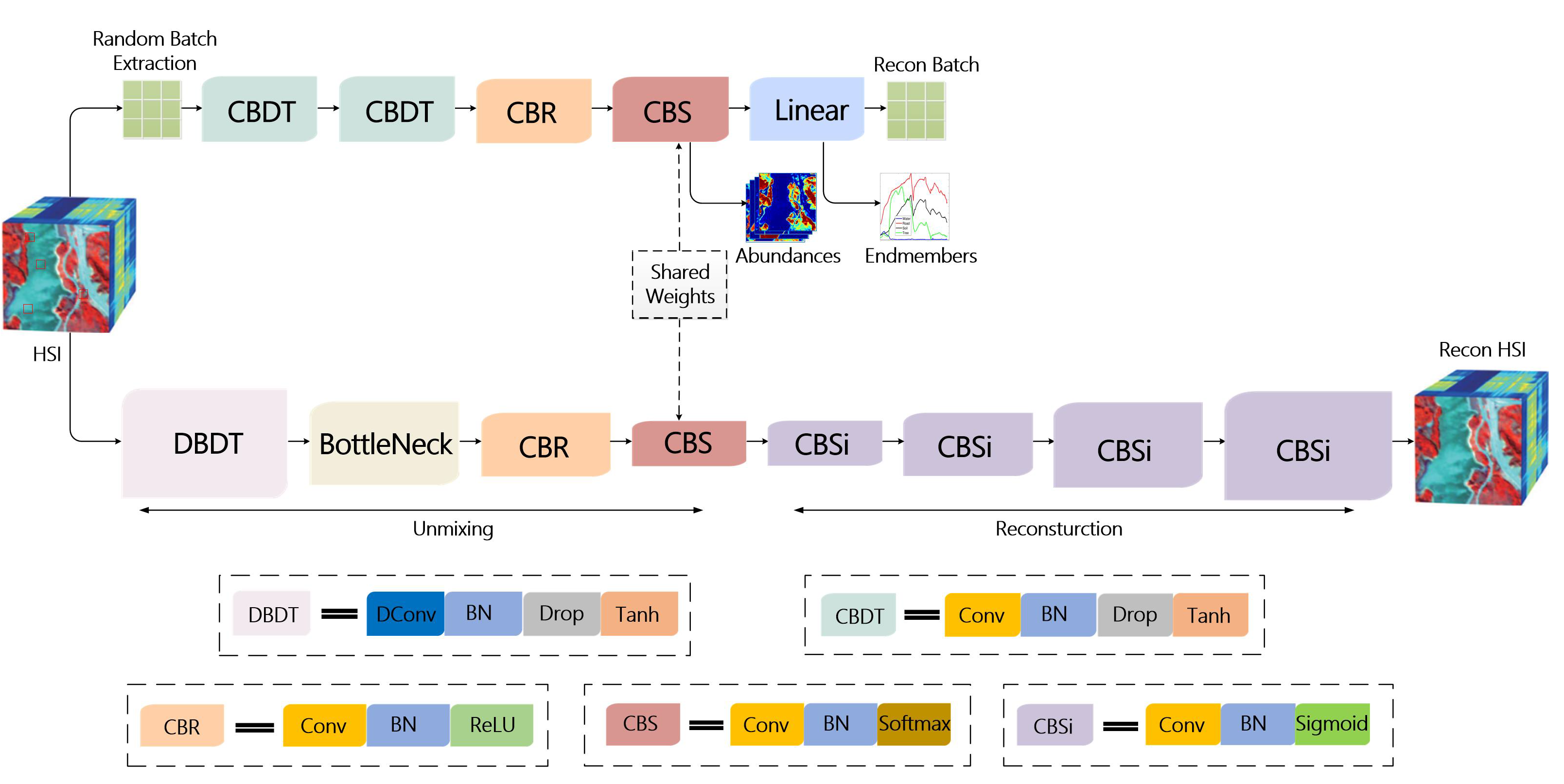
The above methods do not fully exploit the spatial–spectral information and ignore differences in the distribution of endmembers. To solve these problems, in this paper, a spatial-information-assisted spectral information learning unmixing network (SISLU-Net) is proposed. It has two branches. One branch focuses on the extraction of spectral information, where the HSI is divided into
pixels, and a random combination of several pixels is selected each time and sent into the network for training. Another branch uses DBDT and residual modules to learn the spatial information of the entire HSI. By sharing the weight, the lower branch can transfer the learned spatial information to the upper branch, which helps the upper branch network to better unmix the data [
32]. Considering that the distribution of endmembers presents different problems, we employ a new loss function to deal with situations where there are different data distributions. More specifically, the contributions of this paper can be elaborated as follows:
(1) We propose an end-to-end two-branch network structure called SISLU-Net for HSI unmixing. The two branches collaborate on HU by sharing weights. Through the shared weight strategy, the lower branch transfers the learned spatial information to the upper branch, which then assists the upper branch to estimate the abundance and endmembers effectively and accurately.
(2) The main purpose of the upper branch of the network is to learn spectral information. Due to the similarity of adjacent regions, pixels from each region are extracted as randomly as possible from the global scene and transported into the network. Thus, the learned spectral information is more diverse and accurate.
(3) In another branch of the network, we introduce a bottleneck residual module, which combines low-level features with high-level features to achieve feature multiplexing. In addition, in the DBDT module, the dilated convolution obtains context information in a dilated manner, thus avoiding only learning local similar spatial information and making the network more comprehensive.
(4) Wing loss is employed as a new loss function in the proposed SISLU-Net. Wing loss is better compatible with data outliers and therefore able to solve the problem of differences in the distribution of endmembers. Experiments on the Samson and Jasper Ridge data sets verify the superiority of the proposed Wing loss compared to several commonly used loss functions.


