Article

Urbanization Trends Analysis Using Hybrid Modeling of Fuzzy Analytical Hierarchical Process-Cellular Automata-Markov Chain and Investigating Its Impact on Land Surface Temperature over Gharbia City, Egypt

1
Department of Earth & Environmental Science, Institute of Global Environmental Change, School of Human Settlements and Civil Engineering, Xi’an Jiaotong University, Xi’an 710049, China
2
Geomatics Engineering Department, Faculty of Engineering at Shoubra, Benha University, Banha 13511, Egypt
*
Author to whom correspondence should be addressed.
Remote Sens. 2023, 15(3), 843; https://doi.org/10.3390/rs15030843
Submission received: 22 November 2022 / Revised: 28 January 2023 / Accepted: 30 January 2023 / Published: 2 February 2023
(This article belongs to the Special Issue Urban Planning Supported by Remote Sensing Technology)

Abstract

:
Quick population increase and the desire for urbanization are the main drivers for accelerating urban expansion on agricultural lands in Egypt. This issue is obvious in governorates with no desert backyards. This study aims to (1) explore the trend of Land Use Land Cover Change (LULCC) through the period of 1991–2018; (2) upgrade the reliability of predicting LULCC by integrating the Cellular Automata (CA)-Markov chain and fuzzy analytical hierarchy process (FAHP); and (3) perform analysis of urbanization risk on LST trends over the Gharbia governorate for the decision makers to implement effective strategies for sustainable land use. Multi-temporal Landsat images were used to monitor LULCC dynamics from 1991 to 2018 and then simulate LULCC in 2033 and 2048. Two comparable models were adopted for the simulation of spatiotemporal dynamics of land use in the study area: CA-Markov chain and FAHP-CA-Markov chain hybrid models. The second model upgrades the potential of the CA-Markov chain for prediction by its integration with FAHP, which can determine the locations of high potential to be urbanized. The outcomes stated a significant LULCC in Gharbia during the study period—specifically, urban sprawl on agricultural land, and this trend is predicted to carry on. The agricultural sector represented 91.2% in 1991 and reduced to 83.7% in 2018. The built-up area is almost doubled by 2048 with respect to 2018. The regression analysis revealed the LST increase due to urbanization, causing an urban heat island phenomenon. Criteria-based analysis reveals the district’s vulnerability to rapid urbanization, which is efficient for data-gap zones. The simulation results make sense since the FAHP-CA-Markov simulated the LULCC in a thoughtful way, considering the driving forces of LULCC, while the CA-Markov chain results were relatively random. Therefore, the FAHP-CA-Markov chain is the pioneer to be relied upon for future projection. The findings of this work provide a better understanding of LULCC trends over the years supporting decision makers toward sustainable land use. Thus, further urbanization should be planned to avert the loss of agricultural land and uninterrupted increasing temperatures.

1. Introduction

One of the most critical trends of Land Use Land Cover Change (LULCC) is urbanization [1]. This accelerated phenomenon has extremely negative impacts on the environment and socio-economy [2,3]. Awareness of these environmental and socioeconomic problems motivates the subject of the LULCC to be studied. The analysis of urbanization experiences a shortage of knowledge and understanding of the urban expansion process, in addition to the physical and socioeconomic factors [4,5]. This paper considers these limitations and provides upgraded techniques for monitoring and predicting urban sprawl dynamics over the Gharbia governorate, Egypt, for supporting productive and sustainable urban planning. This paper also investigates the direct impact of urban expansion over agricultural lands on the land surface temperature (LST).
Egypt is an agricultural country with highly fertile soil [6]. However, at this time, the agricultural land area continues to decrease, specifically in the governorates with no desert backyard [7]. With overpopulation, no direct reaction except urban sprawl over agricultural lands is expected [8]. Thus, the negative impact of urbanization is multiplied: (1) overpopulation in a way that is incommensurate with the resources, leading to water scarcity and air quality reduction [9,10]; and (2) food shortage crisis as the per capita share of agricultural land is shrinking. The Gharbia governorate is a live model of this issue.
Satellite remote sensing has become a growingly robust and efficient tool for monitoring and mapping land cover [11]. The potential of mapping urbanized areas has been improved thanks to the various updates in sensor technology. The classification of satellite images for obtaining land cover categories [12] is almost the most substantial avail of digital image analysis. The classification techniques are categorized as supervised or unsupervised. Supervised classification is preferable since the algorithm classifies the image based on training samples for each land cover defined by the user. There is a diversity of supervised classifiers, e.g., maximum likelihood classification (MLC); support vector machine (SVM); decision tree; logistic regression; and so on. In the MLC, a pixel with the maximum probability is grouped into the matching class. Otherwise, SVM is a kernel-based algorithm that begins working with comparatively low-dimension data and then upgrading them into a higher dimensional space and getting a higher dimensional support vector classifier that enables the observations classification successfully [13,14,15].
For the simulation of LULCC dynamics, various models are available, e.g., SLEUTH [16], SERGoM [17], GEOMOD [18], Dinamica [19], and Cellular Automata—Artificial Neural Network (CA-ANN) [20]. SLEUTH, for instance, extrapolates the future LULCC according to the land use behavioral change [21] but it requires parameter values to be known in advance. Baig et al. [22] assessed the LULCC and predicted future trends in Selangor, Malaysia based on the CA-ANN model. The urban area has increased while the green cover has decreased accordingly, and the prediction results confirmed a persistent decrease in agriculture and forests opposite to the increase in built-up areas. Otherwise, the Markov chain is a stochastic model which is capable of estimating transition potentials of land use without determining such transitions spatially [23,24]. The Markov chain algorithm can be integrated with such spatial models of LULCC to estimate the location and quantification of conversions relying on historical Land Use Land Cover (LULC) trends [25].
Many previous studies have monitored and simulated the urban expansion trends using the CA-Markov chain model and their results were satisfying and compatible [25]. For instance, Wang et al. [26] addressed the LULCC detection and prediction in Bhutan’s high-altitude city of Thimphu, using the CA-Markov chain. The study recorded a considerable increase in urban area, followed by an insignificant increase in barren ground cover during the interval of 2002–2018. Contrarily, the forest class decreased dramatically followed by agricultural land. Simulation results expected a persistent trend of land cover change until 2050. Moreover, Koko et al. [27] adopted the CA-Markov chain to predict the LULCC in Kano Metropolis, Nigeria over 2035 and 2050 based on the past trends of the period of 1991–2020. The hybrid model skipped the limitations of each individual model. Samat et al. [28] also simulated the spatiotemporal LULCC in Malaysia’s conurbation using the CA-Markov chain model and GIS technique. Further recent studies that employed the same model to predict future land uses were performed in the Atlanta Metropolitan area of Georgia, USA [29], Jiangle County, China [30], and Changping District in Beijing, China [31]. These studies have shown the superiority of the CA-Markov model in simulating LULC transition and confirmed its capability for better extrapolating future land uses.
On the other side, in this research, a hybrid model of fuzzy analytical hierarchy process (FAHP), CA, and Markov chain has been addressed for more accurate simulation and forecasting of LULCC. This hybrid model adopts the concept of multi-criteria decision-making (MCDM) through the FAHP. Based on selected criteria represented mainly in the urban sprawl parameters, the locations highly susceptible to LULCC can be identified. This integration will provide a better understanding of urbanization patterns to assist the decision makers in developing sustainable urban planning in the future. FAHP was utilized to obtain the transition potentials which can be integrated with that from the CA-Markov chain, which will then be conducted on the LULC maps of 1991, 2003, and 2018 to predict the future LULC of 2033 and 2048. Therefore, the results of the prediction are supposed to be more logical since the prediction manner considers the major drivers of LULCC. Furthermore, this work depends on the fuzzy MCDM which can dispose of uncertainty in data and analysis, contrary to the usual use of MCDM techniques by researchers.
Furthermore, the LSTs of the study area over the study period were extracted from the thermal bands of the selected Landsat images. Pal and Ziaul [32] studied the effect of LULC type on LST based on multi-temporal satellite images. The findings showed a considerable LST variation present over diverse LULC types and the built-up area had maximum LST. A high correlation between LST and LULC type was observed indicating that the impervious surfaces maximally control LST, followed by water bodies and vegetation. Therefore, the LULCC pattern affects LST and air temperature. It means the accelerated urban expansion negatively impacts the climate status, like the appearance of the UHI phenomenon. This issue was addressed by Effat et al. [33] who focused on monitoring the trends of urbanization and UHI in Tanta city, Egypt, based on multi-temporal remote sensing (RS) data and GIS. The LSTs, retrieved from the thermal bands, were analyzed to detect the phenomenon of UHI. Otherwise, the LULC maps were gained based on image classification. Then, a regression analysis was conducted to reveal the relationship between the LST and the different classes of land use, particularly agricultural and urban areas. The findings illustrated a massive urban expansion at the expense of the agricultural area, leading to a growing UHI intensity. The regression analysis revealed that the LST increases with the spread of urban class and decreases with green space.
The recognition of LULCC patterns and related motives is critical to promote ideal urban strategies which can ensure economic, social, and environmental sustainability [7]. Accordingly, this study focuses on three primary objectives: (1) monitoring the trend of LULCC through the period of 1991–2018; (2) simulating LULCC by 2033 and 2045 based on a hybrid model of CA-Markov chain and FAHP; and (3) analysis of urbanization risk on LST trends across the Gharbia governorate for the decision makers to implement effective strategies for sustainable land use. The outcomes of this paper provide a better understanding of LULCC dynamics over the years and suggest that thinking of new urbanism should be planned to avoid persistently elevated temperatures.

2. Materials and Methods

2.1. Study Area

Gharbia settles in the middle of the Nile delta of Egypt at 30.87°N lat and 31.03°E long. It is bounded by the two branches of the Nile river to the east and west as exhibited in Figure 1. The area of the Nile delta is one of the oldest agricultural lands in the world where agricultural activity has been practiced continuously for more than 5000 years [3,34]. The Nile river made the delta soil highly fertile and accordingly elevated crop production, generating an evident green triangle enclosed by a vast desert.
Agriculture as an LULC category is dominant in the governorate of Gharbia, which is used to planting conventional yields such as potatoes for domestic consumption and export, as well as strategic crops such as rice, grains, and high-quality cotton. Furthermore, this governorate contributes 86% of Egypt’s flax production. This governorate involves eight territories as elucidated in Figure 1, covering 1999 km2. The population density was estimated in 2018 as almost 5,066,000 persons, whereas it was hardly 4,011,320 and 3,790,670 in 2006 and 2001, respectively. Our study focused on such areas suffering from accelerating urban sprawl on agricultural lands, resulting in food security challenges and LST increase.

2.2. Data Collection and Processing

Multi-temporal Landsat images were employed in this article. Landsat has been relied upon due to its rich and free archive that allows long-term study. To gain the LULC maps for the study years, Landsat 5 TM was utilized for 1991 and 2003 while Landsat 8 OLI/TIRS was utilized for 2018 [36], and then, land cover change was deduced through time [37]. The selected images were clear without cloud spectrum by dint of a dry summer season since all images were captured in June. For image preprocessing, atmospheric correction was performed for each captured image. Six images were collected since the area of interest is located in two shots. Then, mosaic was applied and the mosaicked images were subset by the study area. These images were selected to be in the same season for a more realistic comparison over the years. The free source of open street map (OSM) was relied upon to acquire the road network of the study area for extracting a “distance from nearest road” layer for later use. Based on Google Earth historical images, training samples used for supervised classification and test samples used for classification assessment were obtained (as mentioned in Table 1).
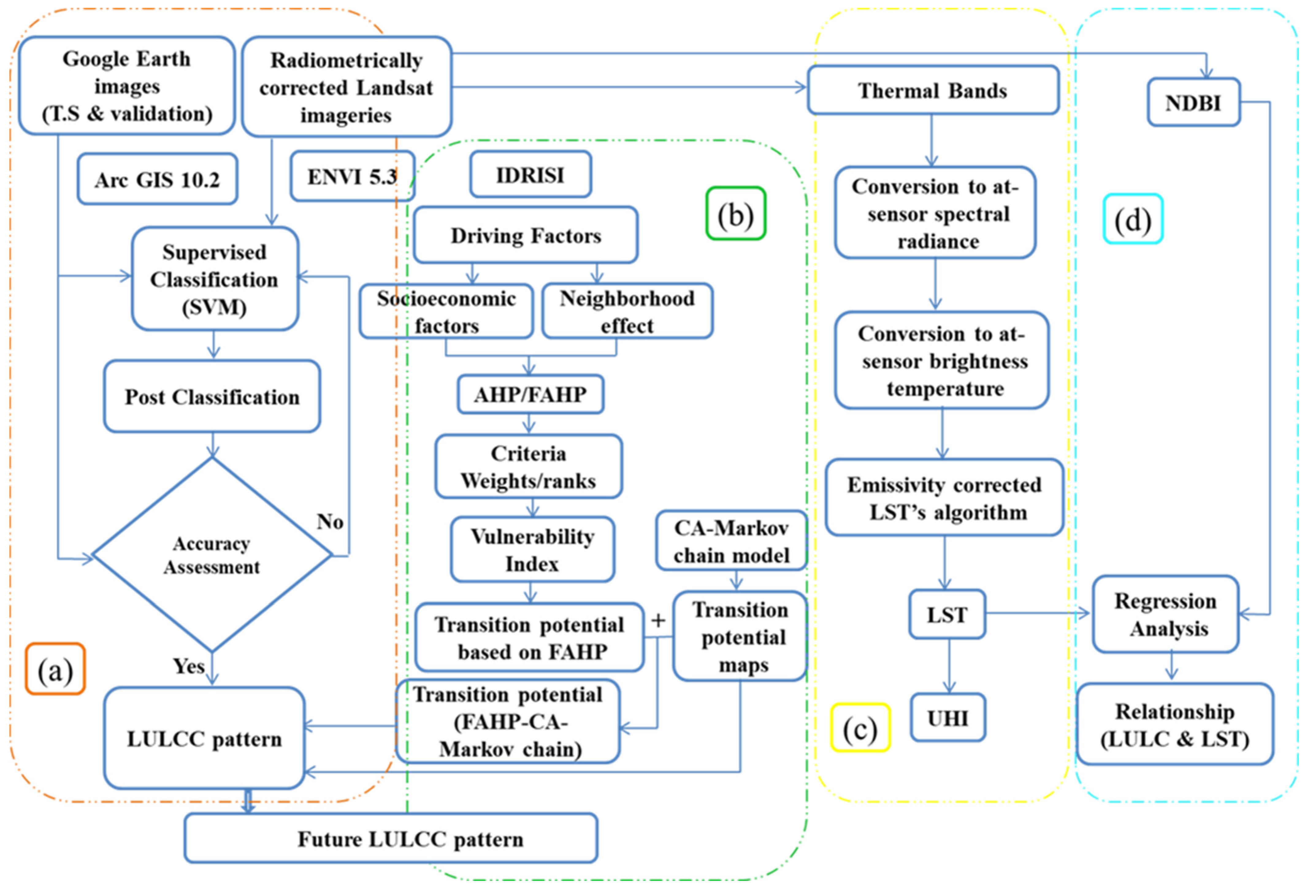
After the image preprocessing, the images are prepared for further processing as shown in Figure 2. Figure 2 demonstrates the flowchart of the adopted methodology to monitor and simulate the LULCC in the present and the future based on comparable models, with four primary steps.

2.3. LULC Classification

Our study area has three types of LULC: built-up, water, and agricultural land. Based on [35], Landsat images of the study area were classified using supervised classification techniques; MLC as a parametric pixel-based method compared to SVM classification as a non-parametric pixel-based technique [38]. However, SVM was superior to be relied on than the MLC as it can be visually noticed that the SVM-based classified image simulates the real land cover frequently better than that of the MLC-based. Therefore, SVM was adopted to extract the present LULC classes from the satellite images.
As usual, there were some misclassifications in the initial outputs of the classification step. Accordingly, a majority filter was employed to minimize the noises from the spectral confusion [39]. Namely, the classification accuracy can be raised through post-classification improvement.
To guarantee accurate change detection, classification accuracy needs to be assessed. The most popular approach for the accuracy assessment of classified images is called the error matrix [40]. The error matrix compares the classified image with its reference image on a class-by-class principle. A random sampling method [41,42] was utilized to spread 1000 checkpoints for every image covering all LULC types in a well-distributed manner, to fulfill more actual classification accuracy [43]. Based on the confusion matrix, overall accuracy (OA %) was computed to estimate the classification accuracy. However, OA is incapable of revealing whether the errors were reasonably extended among categories or whether some categories were really bad and some were really good. So, three indices of accuracy were computed as well: user’s accuracy (%); producer’s accuracy (%); and kappa coefficient [44,45].

2.4. LULC Change Modeling

Generally, the LULCC modeling process includes three major phases: (1) model calibration; (2) model simulation and validation; and (3) model prediction.
(1)
Model Calibration
The model was calibrated for pixels that transferred from every LULC type to all other types in the first study period of 1991–2003. Accordingly, the transition potentials can be defined quantitatively and/or spatially based on the model used.
(2)
LULC Simulation and Model Validation
After the calibration step, LULC for the year 2018 was simulated based on the observed trends pending the calibration interval (1991–2003). Then, the simulated 2018 LULC map was compared to the observed one, extracted previously based on the SVM-supervised classification of the Landsat image, for model validation. The model validation was employed to assess the performance of the model to be used in simulating and then predicting future LULC maps [46,47]. Cohen’s kappa coefficient [48] is an index for the model assessment. It ranges from zero to one. Low values of kappa (0 to 0.2) express the inconsiderable relationship between the compared maps while high values (0.81 to 1) refer to almost perfect coincidence [49,50]. However, we relied on another index for evaluating the model simulation capability since the kappa statistic introduces an overall estimation and lacks a cross-check of results [51]. The Jaccard similarity coefficient was preferred for the verification of the results [50]. The Jaccard coefficient is a measure of similarity for two data sets, ranging from 0% to 100% indicating the degree of agreement between the two sets. The higher the percentage, the more similar the two sets are. The threshold for acceptable Jaccard coefficients is 60%. The Jaccard coefficient can be computed as the ratio of the area of intersection between the two layers (simulated and actual) versus their union area [35] as clarified in Equation (1), where 0% reveals no intersection between the actual and simulated change while 100% refers to typical coincidence. Since the most remarkable transition is urban encroachment on agricultural land, the observed and simulated land use of built-up for 2018 was extracted to calculate the Jaccard coefficient.
J c ( simulated , observed ) 2018 =   simulated   urbanization observed   urbanization   simulated   urbanization observed   urbanization
(3)
Model Projection
The last stage of the modeling process after the calibration and validation steps is the projection of the LULCC in the future. Once the model succeeds in the validation step, it can be adopted to predict the LULC in 2033 and 2048. The predicted transitions of LULC were extrapolated based on the simulation period (2003–2018). So, in this step, the input data images were updated to the actual LULC 2003 and 2018, not the simulated ones. In this article, the modeling process has been applied based on two comparable models.

2.4.1. CA-Markov Chain Model

A CA-Markov chain model is an integration of the Markov chain stochastic model and the spatial model of CA. The “transition potentials” can be extracted based on the Markov chain stochastic model, whereas the CA spatial model determines the transition potential maps. The CA model acts as an urban area with a network of cells, each of which exists in one of a finite set of states. The state of a cell relies on the states of its neighbors and changes as a function of time. The progression of time is formulated as a chain of discrete steps with future patterns determined by transition rules which assign the attitude of cells over time [52]. The Markov chain depicts a series of states in which the chance of each state relies just on the acquired trend in the prior state. For clarification, the Markov chain has n states. The state vector is a column vector whose ith component represents the probability that the system is in the ith state at that time. Note that the sum of the entries of a state vector is 1 [52,53,54]. Markov theory gives the relation between two sequential state vectors; for example, if Xn+1 and Xn are two successive state vectors of a Markov chain with transition matrix T, then
X n + 1 = T × X n
The IDRISI Sleva (geospatial monitoring and modeling system) from Clark Lab (Clark University, Worcester, MA, USA) is the software for simulating land use change and CA-Markov analysis. The CA-Markov analysis was applied to examine a pair of land cover images and to output transition probability and transition area matrices. The first matrix is the probability of moving from one state to another during one time period, whereas the second one is the number of pixels that are expected to change from each land cover type to every other one over a particular number of time units. In our case, the time step is almost 15 years where we first depended on the images captured in 1991 and 2003 to process the model to simulate 2018 which has been already pre-captured. After validating the model, the CA-Markov Chain model was utilized to project the LULC in 2033 and 2048.

2.4.2. FAHP-CA-Markov Chain Hybrid Model

In this model, not only CA-Markov was relied upon, but also the MCDM technique, specifically the analytical hierarchy process (AHP), was involved. In other words, the traditional CA-Markov chain model is intended to be improved or upgraded by its integration with MCDM techniques to obtain a better and more accurate transition potential map. Therefore, the hybrid model of AHP and CA-Markov chain models has considered the merits of the traditional CA-Markov chain model in addition to the substantial feature of the MCDM techniques for more accurate simulation and projection of LULCC.
The AHP is a technique for controlling and analyzing complicated decisions, utilizing math and psychology. It was developed by Thomas L. Saaty in the 1970s and has been revised since then [55]. Stakeholders compare the significance of criteria, two at a time, through pairwise comparisons. AHP transforms the evaluations into numbers, which can be compared to all of the potential criteria. This quantifying ability discriminates the AHP from other decision-making techniques. In the last step of the process, numerical preferences are calculated for all the alternative choices. These numbers show the most required solutions, based on all users’ values.
As we mentioned, the MCDM is capable of assigning the locations of a high probability of susceptibility to LULCC through the study area based on selected criteria. Therefore, to monitor and predict the LULCC, specifically the urbanization, the selected criteria were represented in the urban sprawl parameters or the driving factors contributing to urban expansion: socioeconomic parameters and neighborhood effect, in addition to the type of land use itself. Therefore, the hybrid model of the AHP-CA-Markov chain is capable of predicting the locations susceptible to urban sprawl in a systematic way. Otherwise, FAHP is a method of AHP [56] developed with fuzzy logic theory. We applied this integration with both AHP and FAHP. However, the fuzzy model of AHP was preferred over the AHP to overcome uncertainty in data and analysis. The used fuzzy numbers were extracted based on the triangular membership function [57,58]. In the previous section, the concept of the CA-Markov chain model was mentioned, so here we focus on what concerns the FAHP model.
a.
Driving factors
There are various factors that directly or indirectly drive urban expansion. It is critical to identify and understand the impacts of these factors on LULCC for sustainable urban planning and management strategies [59,60,61]. Previous studies have dealt with diverse factors and their influences on urbanization. The selection of the factors usually depends on the properties of the study area, understanding of LULCC over time, and expert awareness of assorted study areas [62,63]. Therefore, based on our knowledge of the study area and considering the development pattern of the area, we adopted socioeconomic factors, neighborhood effect, and LULC type. The socioeconomic factors are the most significant factors of urban growth involving: “distance to persistent built-up area”, “distance to urban centers”, “distance to railway stations”, “distance to nearest road”, “population density”, “employment”, and “local development”. The natural factors such as slope and elevation can be negligible since the area of interest is almost level.
b.
Steps of applying the FAHP model [64] based on the aforementioned criteria:
The fuzzified pairwise comparison matrices (FPCMs) are obtained by comparing all the possible pairs of criteria to rank the criteria in order of priority. Every element takes a value from 1 to 9 based on its significance, the value of 1 refers to the criteria being equally important while a value of 9 expresses that the considered criterion is exceedingly important compared to the others. This is called scaling. FAHP is performed through the following eight steps: (1) Formation of the fuzzified pairwise comparison matrix as follows:
à = ( ã ) n × n = [ ( 1 , 1 , 1 ) ( l 12 , m 12 , u 12 ) ( l 1 n , m 1 n , u 1 n ) ( l 21 , m 21 , u 21 ) ( 1 , 1 , 1 ) ( l 2 n , m 2 n , u 2 n ) ( l n 1 , m n 1 , u n 1 ) ( l n 2 , m n 2 , u n 2 ) ( 1 , 1 , 1 ) ]
(2) Calculating the fuzzy synthetic extent with respect to ith alternative using the following Equation (4):
s i = j = 1 n a i j [ i = 1 n j = 1 n a i j ] 1
where aij is the element of the FPCM of n: no. of criteria.
(3) Calculating the degree of possibility for a convex fuzzy number to be greater than k convex fuzzy numbers:
V ( s 1 s 2 ) = s u p y x [ min ( μ s 1 ( x ) , μ s 2 ( x ) ) ] = h g t ( s 1 s 2 ) = { 1 if   m 1 m 2 , 0 if   l 2 u 1 , l 2     u 2 ( m 1     u 1 )     ( m 2 l 2 ) ,   o t h e r w i s e V ( S S 1 , S 2 , S 3 , S k ) = min V ( S S i ) , i = 1 , 2 , k
(4) Calculation of the weight vector and normalize the nonfuzzy weight vector.
d ( A i ) = min V ( S i S k ) , W = ( d ( A 1 ) , d ( A 2 ) , , d ( A n ) ) T
(5) Computing λmax (the principal eigenvalue).
(6) Estimating the consistency index (CI) to measure the inconsistencies of pairwise comparisons using Equation (7):
C . I . = λ max n n 1
where n is the number of criteria and λmax is the highest eigenvalue [65].
(7) Determining the appropriate value of the random consistency ratio (RI). RI values are illustrated in the Supplementary Material (Table S1).
(8) Calculating the consistency ratio (CR) by the following relation (Equation (8)):
C R = C I R I
We have depended on nine criteria, so the fuzzified pairwise comparison matrix was created as elucidated in Table 2. According to the authors’ prior knowledge of the study area, the criterion of “distance to persistent built-up areas” has the highest significance, so it was given the value of 9. Likewise, all the other criteria weights and their ranks were estimated to determine the locations of high potential to LULCC.

2.5. Estimation of Land Surface Temperature

2.5.1. LST Estimation from Landsat Imageries

The LST can be extracted from the thermal bands of the satellite data images. In Landsat 5 TM, band 6 represents the thermal band while there are two thermal bands (band 10, 11) in Landsat 8 OLI/TIRS. However, we relied only on band 10 since the USGS recommended that band 11 should not be used for LST estimation due to the effect of stray light in Landsat 8 TIRS.
The digital numbers of the thermal bands of the satellite imagery were converted to at-sensor spectral radiance. This transformation was performed by applying the following equation [66]:
L λ = ( LMAX λ   LMIN λ Qcalmax Qcalmin ) ( Qcal Qcalmin ) + LMIN λ
where:
  • L = spectral radiance at the sensor’s aperture (Watts m−2 sr−1 μm−1);
  • Qcal = the quantized calibrated pixel value in DN;
  • LMINλ = the spectral radiance scaled to QCALMIN in (Watts m−2 sr−1 μm−1);
  • LMAXλ = the spectral radiance scaled to QCALMAX in (Watts m−2 sr−1 μm−1);
  • Qcalmin = the minimum quantized calibrated pixel value (corresponding to LMIN) in DN;
  • Qcalmax = the maximum quantized calibrated pixel value (corresponding to LMAX) in DN.
Once the DNs for the thermal bands were turned into Top of Atmosphere (TOA) radiance values, the brightness temperatures can be estimated using this formula of Artis and Carnahan [66]:
T B ( ° K ) = k 2 ln ( [ K 1 L λ ] + 1 )
where:
  • TB—is the satellite brightness temperature in degrees Kelvin;
  • K1_constant_band_6 of TM 5 = 607.76;
  • K2_constant_band_6 of TM 5 = 1260.56;
  • K1_constant_band_10 of TIRS 8 = 774.8853;
  • K2_constant_band_10 of TIRS 8 = 1321.0789;
  • Lλ—is TOA spectral radiance.
Then, the LST was computed by applying the emissivity-corrected land surface temperature’s algorithm [66]:
S t ( ° K ) = T B 1 + ( λ   ×   T B ρ ) ln ε
where:
  • St—is the emissivity-corrected land surface temperature in degrees Kelvin;
  • TB—is the satellite brightness temperature in degrees Kelvin recaptured earlier;
  • λ = 11.457 µm;
  • ρ = h × c δ = 1.438 × 10⁻² m k= 1.438 × 104 µm k;
  • h—is Planck’s constant = 6.626 × 10⁻³⁴ J s−1;
  • c is velocity of light = 2.998 × 10⁸ m s−1;
  • δ is Boltzmann’s constant = 1.38 × 10⁻²³J k−1.
The emissivity-corrected LSTs were firstly estimated in degrees Kelvin, then the temperature values were obtained in degrees Celsius by merely subtracting 273.15. That is:
S t ( ° C ) = S t ( ° K ) 273.15
Retrieving accurate LST is influenced by three factors: (1) the impacts of atmosphere on the infrared radiation transfer (e.g., water vapor and clouds); (2) the conjunction of LST and land surface emissivity (LSE) causes a complicated situation of LST retrieval; and (3) sensor type [67]. All the methods of estimating LST assume that the emissivity is known. However, in reality, emissivity has to be determined in conjunction with the LST but the number of unknowns is always more than the number of measurements [68,69]. So, LSE may be computed separately.

2.5.2. Computation of LSE ε

LSE is a proportionality factor that scales the blackbody radiance (Planck’s law) to predict emitted radiance, and it is the efficiency of transmitting thermal energy across the surface into the atmosphere [70]. Accurate LSE is in demand in algorithms of LST for leading simulations of surface energy budgets from which surface temperature in the formula is estimated [68,71].
Several approaches have been utilized to extract LSE from Normalized Difference Vegetation Index (NDVI) values [70,72,73]. In this article, the NDVI Thresholds Method (NDVITHM) was adopted. NDVITHM, which was first introduced by Sobrino and Raissouni [74], uses specific NDVI values (thresholds) to discriminate between soil pixels (NDVI < NDVIS) and fully vegetated pixels (NDVI > NDVIV). For those pixels composed of soil and vegetation (mixed pixels; NDVIS ≤ NDVI ≤ NDVIV), the method uses the simplified Equation (13):
ε λ = ε v λ P V + ε s λ ( 1 P V ) + C λ
where εS and εV are the soil and vegetation emissivities, respectively, PV is the portion of vegetation (also referred to as fractional vegetation cover, FVC); the soil influence is lower with increasing PV, and C is a term that takes into account the cavity effect owing to surface roughness (C = 0 for flat surfaces, as in our case).
PV values are obtained from the NDVI according to Skoković et al. [75] by applying the following form (Equation (14)):
P V = NDVI NDVI S NDVI V NDVI S
Over particular areas, NDVIV and NDVIS values (NDVI for vegetated and soil pixels, respectively) can be extracted from the NDVI histogram. Values of NDVIV = 0.5 and NDVIS = 0.2 were confirmed by Sobrino and Raissouni [74] to apply this method in global conditions. In order to gain harmonic values of PV, it must be set to zero for pixels with NDVI < NDVIS and set to one for pixels with NDVI > NDVIV. When NDVI > NDVIV, the pixel is considered fully vegetated and has been granted a constant value of εV = 0.99. NDVITHM estimates the surface emissivity for pixels of bare soil whose PV = 0 (NDVI < NDVIS) as a function of the sensor red band reflectivity (ρred). The relationship between emissivity and red reflectivity is assumed to be linear, and the coefficients are obtained from laboratory spectra of soils and statistical fits. The reasonable formulae for estimating soil emissivity are shown in Equations (15) and (16) for Landsat 5 and Landsat 8 images, respectively:
ε S = 0.979 0.035 × ρ red
ε S = 0.979 0.046 × ρ red
where, ρred is the red band reflectance.
Accordingly, the NDVITHM can be applied as follows:
ε λ = ε s λ NDVI < NDVI s ε s λ 1 P V + ε v λ P V NDVI s NDVI NDVI v ε v λ NDVI > NDVI v

2.6. Regression Analysis

After retrieving the LSTs of each pixel through the study area, it is urgent to study and analyze the relationship between the LULC types and their corresponding LSTs. Linear regression analysis was applied based on the Normalized Difference Built-up Index (NDBI) values of the pixels in the study area corresponding to their LSTs. NDBI was selected since it can well differentiate between the LULC types, where the higher values of NDBI refer to the built-up land use while the lower values represent the classes of agriculture and water. NDBI can be computed by the following formula (Equation (18)):
NDBI = ( SWIR   NIR ) ( SWIR   +   NIR )
where SWIR is short-wave infrared and NIR is near-infrared. SWIR and NIR bands are, respectively, represented in Band 5 and Band 4 of Landsat 5 data and Band 6 and Band 5 of Landsat 8 data.

3. Results

3.1. Accuracy of LULC Maps

Three land-use types are detected through the classification process: built-up, water, and agricultural land. The category of built-up includes all impervious surfaces such as buildings and roads. The class of water bodies includes the Nile river at the borders of the study area and the canals in the middle of the study area. Table 3 displays the indices of accuracy for each classified image of 1991, 2003, and 2018, represented in OA and kappa coefficient. Moreover, the user’s accuracy and producer’s accuracy for each LULC have been mentioned to reveal whether the misclassification was concentrated in a definite class over the others. The SVM has proven its high classification capability that all classification dates fulfilled high OA of 94.9%, 94.7%, and 94.6% and corresponding kappa coefficients of 0.78, 0.81, and 0.84 for 1991, 2003, and 2018, respectively.

3.2. Spatiotemporal Analysis of LULCC

The LULC maps of the study region for the years 1991, 2003, and 2018 are clarified in Figure 3 from which LULC changes over time can be detected. Table 4 quantifies the estimated area of each class in squared kilometers and percentage for the specified times. As shown, agricultural activity is always prominent but it decreases over time. In 1991, the agricultural land represented 1832 km2 (91.2%) and diminished to 1674 km2 (83.7%) in 2018. Otherwise, the class of water represents the least area (1%) and almost no change through the study period. For the built-up land use, the statistical analysis for the year 2003 exhibited that the built-up area has increased in contrast to the decrease in agricultural land. This expansion through the period of 1991–2003 is not disturbing as it is only about 2%. However, urban augmentation was driven to significant growth (almost 5.5%) in the period of 2003–2018 due to urbanization desire. The built-up class occupied 7.8%, 9.7%, and 15.2% in 1991, 2003, and 2018, respectively, which means that the built-up area almost doubled during the study period.
LULCC analysis detects an increasing prevalence of urbanization throughout the study area. For example, built-up land increased by 36.62 km2 and 110.38 km2 within the 1991–2003 and 2003–2018 time periods, respectively. The percentage of built-up land use has increased from 7.8% to 15.2% (nearly doubled) throughout the whole study period (27 years). The agricultural land revealed a similar (but reverse) trend from 1991 to 2018, since the urban growth was extended over the agricultural land.

3.3. LULCC Modeling, Simulation, and Projection

We have mentioned in the section on the methodology that two models were adopted to simulate, and hence predict, the LULCC: CA-Markov chain model and FAHP-CA-Markov chain hybrid model.

3.3.1. Analysis of the CA-Markov Chain Model

Based on the trend of LULC in the period of 1991–2003, the CA-Markov chain model can forecast the LULC for 2018. Then, the model can be validated by comparing the simulated LULC map for 2018 and the corresponding actual LULC one (obtained from SVM classification). Figure 4 illustrates the projected 2018 LULC based on the traditional CA-Markov chain. The used model proved its capability since the kappa and Jaccard similarity coefficients are 84% and 59%, respectively. The findings are considered acceptable and therefore the model can be relied upon for future simulations.
Based on the concept of Markov probability, the successive state vectors of 1991 and 2003 (transition through time step of 12 years) reveals a transition probability matrix of changing to each other class and an expected transition area matrix. In addition, the CA-Markov model was employed to extract the transition potentials for 2018 (a time step of 15 years, as it was the available cloud-free image) based on the past LULC of 1991 and 2003. The transition probability and transition area matrices for the time steps of 12 and 15 years are illustrated in Tables S5–S8, respectively, in the Supplementary Materials.

3.3.2. Analysis of FAHP-CA-Markov Chain Model

The weights of the nine selected criteria for decision making are computed based on applying AHP and FAHP and are highlighted in Table 5. As clarified, the FAHP ignored the criteria of LULC classes, population density, and local development. Both AHP and FAHP models confirmed that the most important criterion is “distance to persistent built-up area”. However, the FAHP model was preferred over the AHP to avoid uncertainty in data and analysis.
Figure S1 compares the transition potential to built-up extracted based on (a) AHP considering all the nine criteria and (b) FAHP considering only 6 criteria. As elucidated, the AHP-based transition potential map has some noise while the FAHP-based one is certain. Accordingly, the FAHP model was confirmed and adopted to integrate with the CA-Markov model for more efficient transition potential maps. Figure S2 highlights the transition potential to built-up based on the hybrid model of the FAHP-CA-Markov chain for the calibration period of 1991–2003.
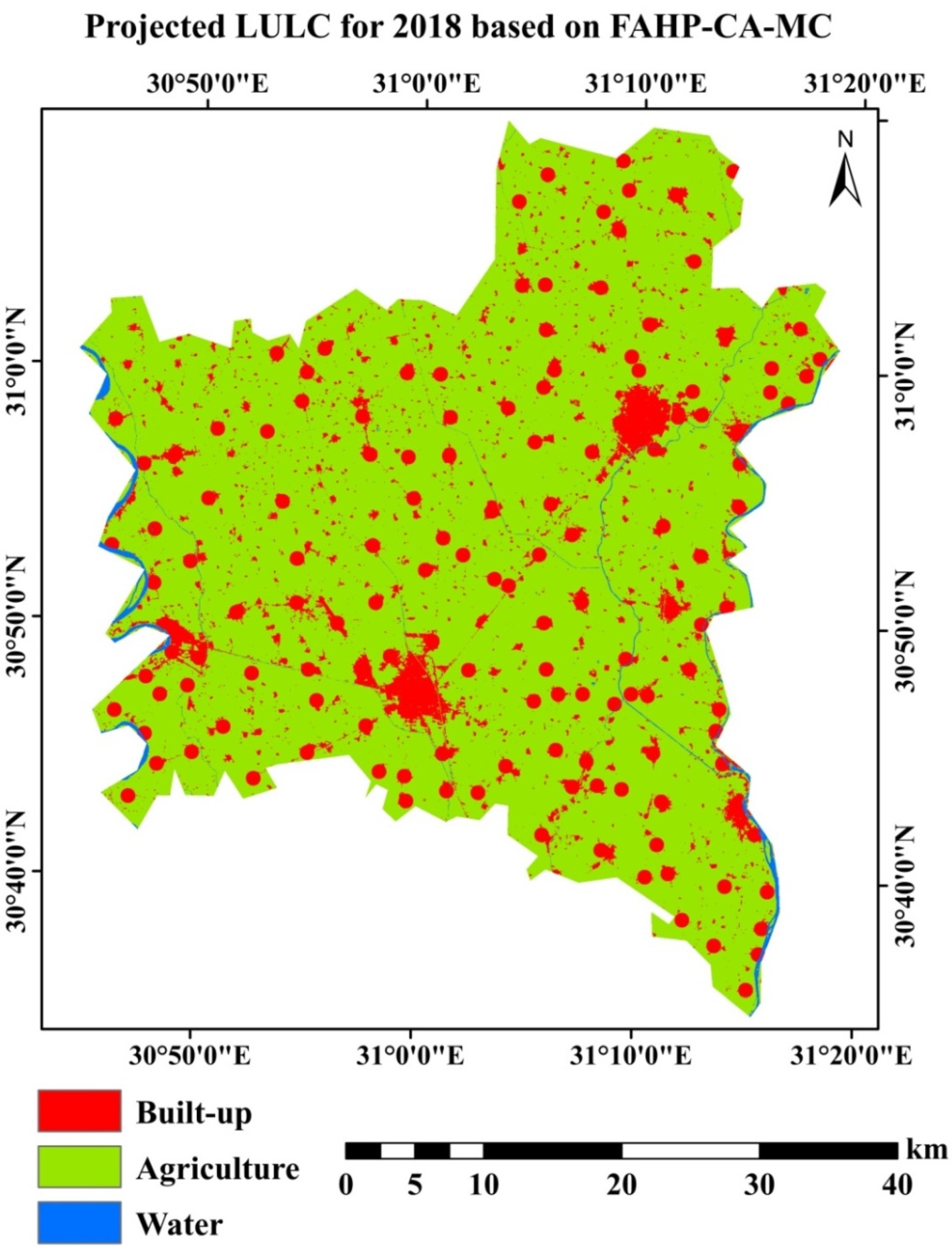
The simulated LULC map for 2018 based on the hybrid model of the FAHP-CA-Markov chain is shown in Figure 5. FAHP played a vital role in defining the locations of high priority to urban growth in a logical way. In other words, the FAHP depends on the driving forces of urbanization which are mainly represented in urban sprawl parameters. The validation of the simulation process based on the hybrid model of FAHP-CA-Markov resulted in a kappa statistic and Jaccard coefficient of 86% and 60%, respectively. The Jaccard coefficient is almost the same in the case of using the CA-Markov model or FAHP-CA-Markov hybrid model.
In the projection phase, the hybrid model was employed to extrapolate future LULC maps for 2033 and 2048 based on the simulation period of 2003–2018. Therefore, the driving factors (criteria) and Markov quantifications have been updated for the 2003–2018 period before running. Figure S3 illustrates the transition potential to built-up based on FAHP-CA-Markov chain hybrid model for the simulation period of 2003–2018 which can be relied upon in the prediction.
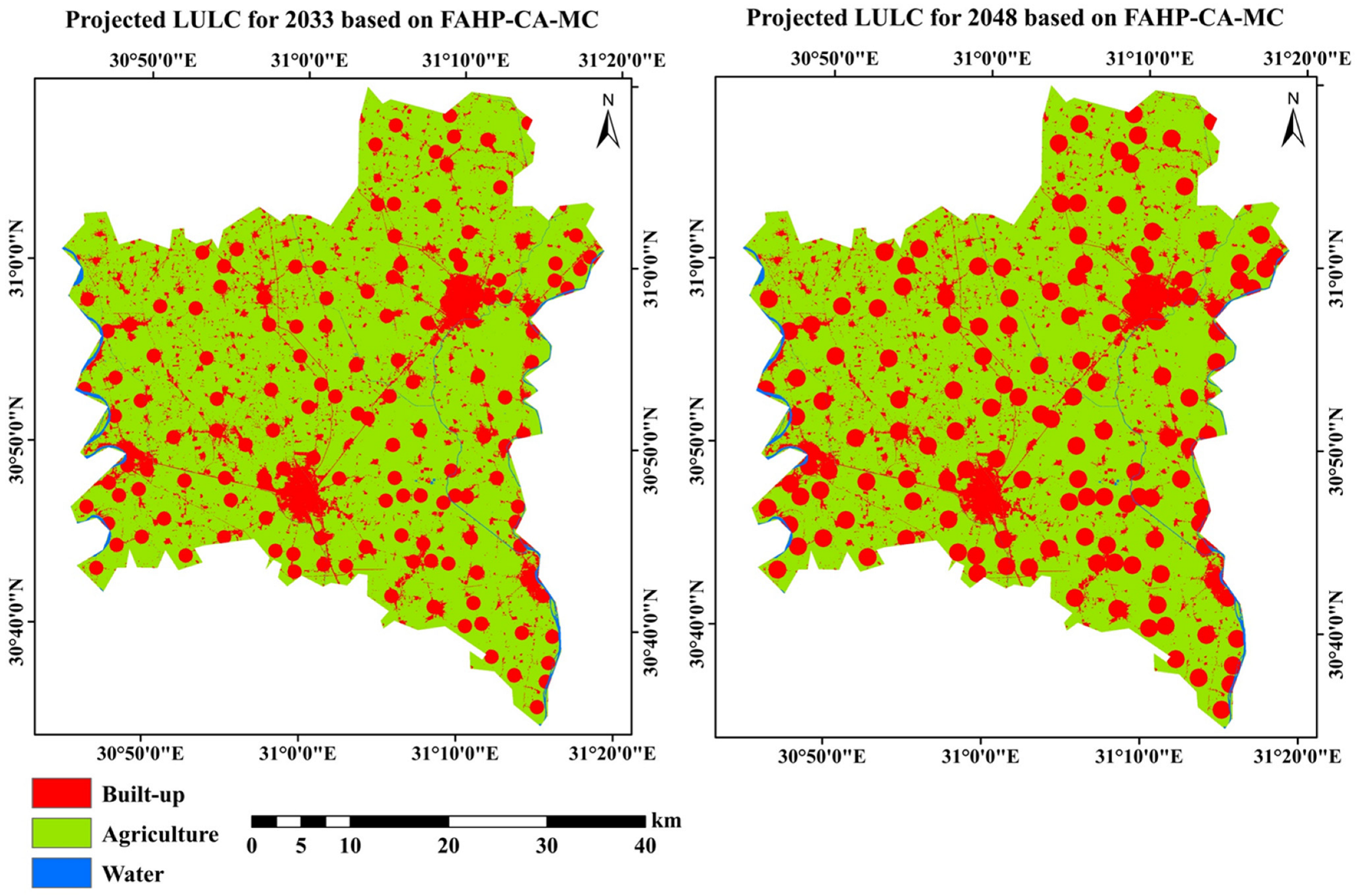
The predicted LULC for 2033 and 2048 emphasized the same trend of persistent urban expansion over the agricultural land as displayed in Figure 6, respectively. Furthermore, the transition probability and transition area matrices were, respectively, stated for 2033 in Tables S9 and S10, and for 2048 in Tables S11 and S12 in the Supplementary Materials, based on the LULC trend of the period 2003–2018. An updated transition potential to built-up based on FAHP-CA-Markov chain hybrid model was obtained for the simulation period of 2003–2018.
Table 6 was created to mention the persistent trend of urbanization at the expense of agricultural land quantitatively over the years. It is found that the built-up area will cover 414.9 km2 and 514 km2 by 2033 and 2048, respectively. It means that the built-up cover will occupy more than one-fifth of the area by 2033 and more than a quarter of the area by 2048. The area of built-up is almost doubled by 2048 with respect to 2018. On the other hand, the area of agricultural activity will decrease owing to the increase in the urban area. It means that the agricultural land will be diminished by the same amount of built-up increase (160.4 km2 and 259.5 km2 by 2033 and 2048, respectively).
This model affirmed the highest weight for the “distance to persistent built-up area”, “distance to urban centers”, and “neighborhood effect”, respectively. Therefore, the maps extracted based on the FAHP-CA-Markov chain model simulated the urban sprawl in a persistent trend around the clusters.

3.4. Analysis of LST

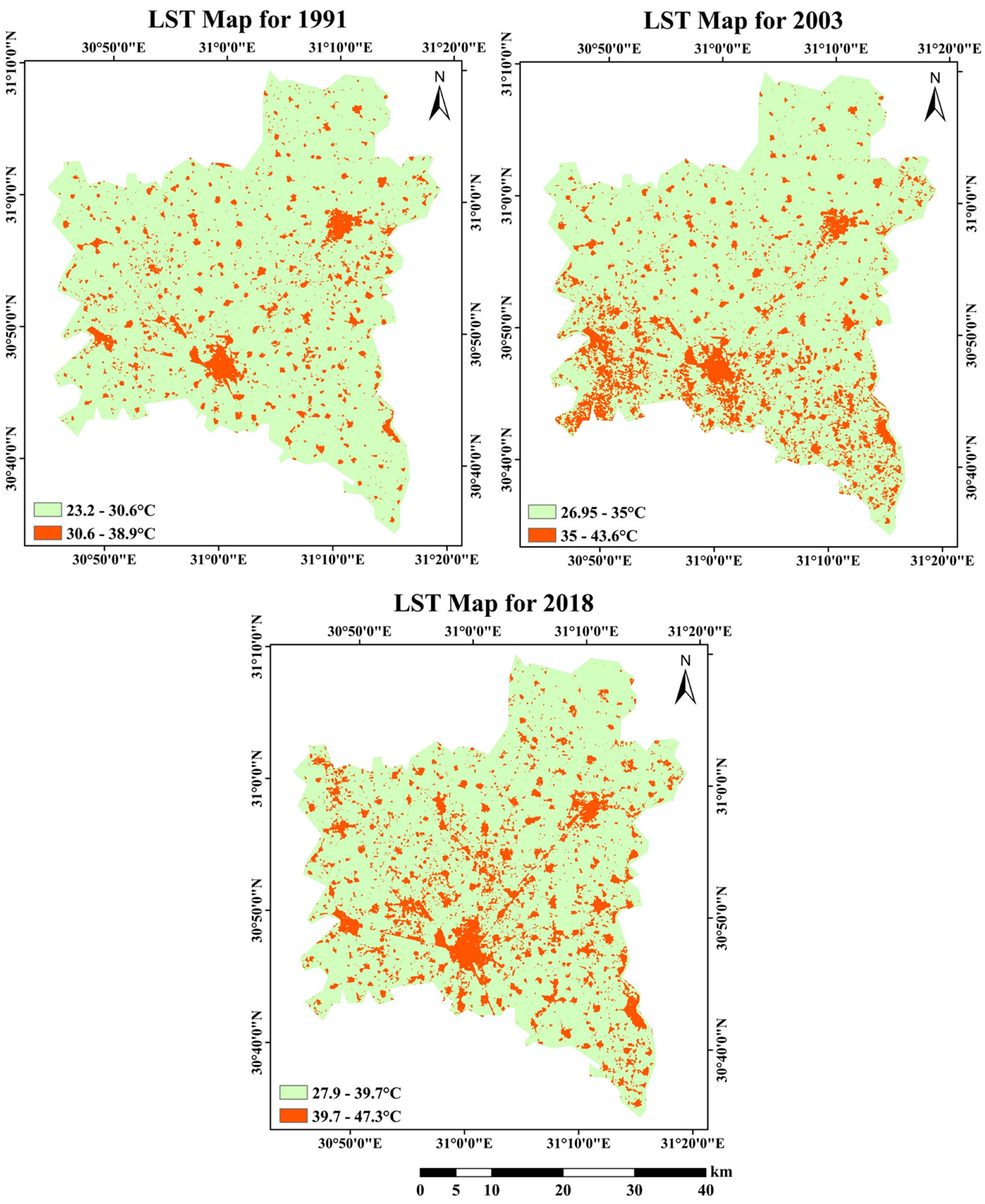
The spatial allocation of the estimated LSTs over Gharbeya city is manifested in Figure 7. LSTs were estimated from Landsat 5 TM band 6 and Landsat 8 TIRS band 10 using the emissivity-corrected land surface temperature’s algorithm. The LST ranged from 23 °C to 52 °C over the study period from 1991 to 2018. It is obvious that the LST for the built-up area is considerably higher than that for agricultural land which signifies the existence of an urban heat island (UHI) effect. The observed effect of the UHI results from a growing population, anthropogenic activities, and LULCC over the study area through the study period. For all the study dates, built-up land use has the highest land surface temperatures while agricultural land and water have the lower.

3.5. Analysis of the UHI

The urban heat islands are urban areas that experience higher temperatures than their neighboring rural areas. To highlight the zones of the UHI, a threshold differentiating the UHI from non-UHI zones is required [76]. Based on Ma et al. [77], the intensity of an urban heat island is defined as the difference between the average temperature of urbanized areas and that of rural ones.
The statistics of LST are summarized in Table S13 in the Supplementary File including the mean LST and standard deviation for the three investigated years. The extracted mean surface temperature for 1991 was 29.47 °C with a standard deviation of 1.89 °C while the mean surface temperatures for 2003 and 2018 were 33 °C and 37.92 °C, respectively, with corresponding standard deviations of 2.59 °C and 3.15 °C. It means there is a persistent trend of LST increase over the years, then the presence of UHIs. The LST mean values for each image were added to half the corresponding standard deviation and considered a threshold to discriminate the UHI from non-UHI zones, as shown in Equation (19) [76]. Temperature values less than the threshold are identified as non-UHI zones. The UHI threshold values are 30.42 °C, 34.30 °C, and 39.50 °C for 1991, 2003, and 2018, respectively.
LST > μ + 0.5 × δ   indicated UHI area LST μ + 0.5 × δ   represented non-UHI
where μ and δ are the mean and standard deviation of temperatures in the study area, respectively. Thus, the UHIs intensities were calculated as the difference between the mean LST of the urban areas and that of the surrounding cultivated areas. The result detected a value of UHI intensity of 3.25 °C, 4.72 °C, and 4.04 °C for the study years 1991, 2003, and 2018, respectively, as shown in Table 7.
The spatial distribution of UHI zones with the corresponding UHI intensities over the study area is shown in Figure 8. The zones of non-UHI appeared in white color and the zones of UHI are classified to express the UHI intensities.
For more productive analysis, the UHI intensity was computed on a district basis to realize the trend of change in LST over each time step on a small scale to specifically define which districts were affected more for the decision maker to adopt for minimizing the UHI impact. According to the intensity of the UHI, Table 8 summarizes the urban LSTs and cultivated LSTs for the eight districts during the study period.
Based on Table 8, there is a fluctuating trend of the UHI effect through all districts of the study area over the study years with the highest UHI intensities in 2003 compared to 1991 and 2018. It seemed that there was a heat wave in 2003 causing this year to have the highest intensities of UHI. The Mahalla Kubra district has noticed a persistent UHI effect with different intensities over the study period of 3.51 °C, 5.53 °C, and 4.37 °C in 1991, 2003, and 2018, respectively. This district has the absolutely highest UHI intensity in the three study years, which means being the most susceptible to the impact of urban expansion as mentioned in Mostafa et al. [35]. Kafr Elzayat has the second-highest UHI in 1991 after Mahalla district but the lowest UHI in 2003 and 2018. For the district of Tanta, the center of Gharbeya city, the UHI intensities were 3.10 °C, 4.65 °C, and 3.91 °C in 1991, 2003, and 2018, respectively. On the other hand, the lowest UHI effect is found in Basun in 1991.
Table S15 represents the mean LST and the standard deviation for each district in the three dates of study which were used to compute the thresholds which differentiate the non-UHI regions from the UHI ones. The eight figures (Figures S5–S12) represent the UHI spatial distribution through the eight districts. The pixels of white color represent the non-UHI where these pixels have LSTs less than the threshold selected based on Equation (4). On the other hand, the pixels of LSTs higher than the threshold model of the UHI zones are classified based on their temperatures for spatial and visual representation. Figures S5–S12 represent the dimensions and the corresponding LSTs for the districts of Mahalla Kubra, Tanta, Zefta, Kafr Elzayat, Qotur, Samanod, Basun, and Santa, respectively. In the figures, a, b, and c represent UHI intensities in 1991, 2003, and 2018, respectively, while d, e, and f are the zoom on the most densely populated area for more clarification of the spatial distribution of LST ranges.

3.6. Relationship between LULC and LST

To quantitatively study the relationship between the land-use types and the surface temperature, regression analysis was employed to statistically analyze the impact of LULCC on the LST change increasingly or decreasingly causing the phenomenon of UHI or UCI (urban cool island).
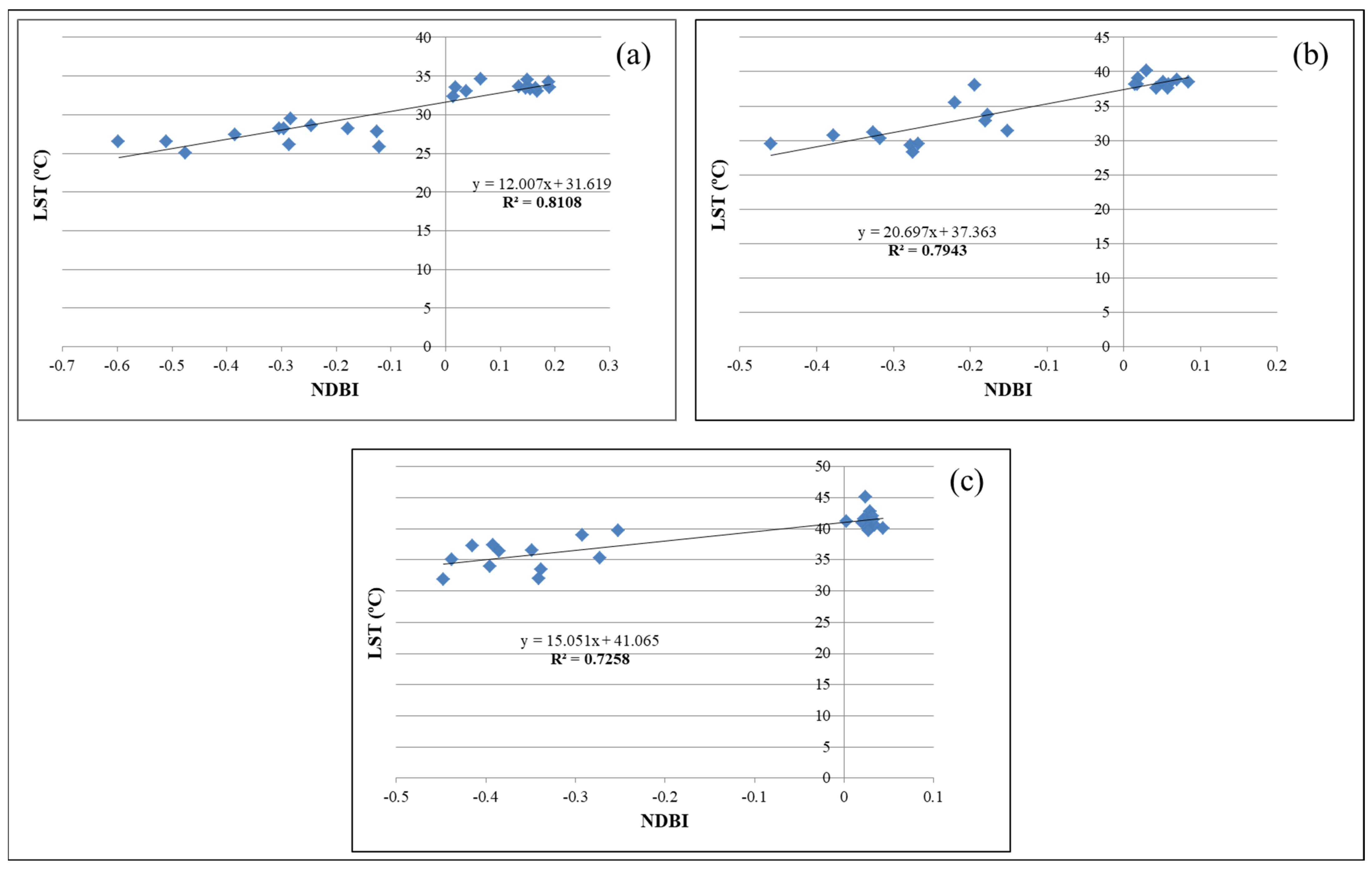
The regression analysis between the LULC and the LST was conducted based on the NDBI values of pixels in the study area corresponding to their LSTs. As shown in Figure 9, there is a positive strong correlation between NDBI and LSTs for all the dates. The linear regression analysis confirmed correlation coefficients of 0.81, 0.79, and 0.73 for the years 1991, 2003, and 2018, respectively.
It is known that the higher values of NDBI refer to the built-up land use while the lower values represent the classes of agriculture and water. So, the high temperatures are always associated with the built-up areas and the agricultural lands and water bodies manifested a considerably low radiant temperature. Therefore, the expansion of urban areas increases the LSTs leading to the effect of UHI. In other words, the increase in LST primarily relied on LULCC, specifically the urban sprawl at the expense of agricultural land. The increase in LST depends on the presence of impervious surfaces such as buildings and roads which keep heat, so the UHI effect is common in cities.

4. Discussion

4.1. Current Study Compared to Previous LULC and Corresponding LST Studies

SVM confirmed its high capability of classification where all classification dates fulfilled high values of classification indices. However, there may be some misclassified pixels; some water pixels for canals were classified as agricultural land since the width of the canals in the study area does not exceed 12 m, and as such these canals are usually edged on both sides by green grass (as shown in Figure S14 in the Supplementary Materials) whereas the Landsat spatial resolution is 30 m. So, these pixels are mixed pixels. For enhancing the classification of the mixed pixels, finer resolution satellite data are required. Sentinel-2 launched in 2015 provides free satellite data with a high spatial resolution of 10m for VNIR and a high temporal resolution of 3–5 days with two satellites [78,79] which are practical for extracting fine features such as streets and canals [80]. However, its short archive lacks the monitoring of spatiotemporal LULCC over a long-term period. In our case, Landsat is considered the most convenient to monitor and assess the phenomena which relate to LULCC since it has the longest uninterrupted RS images of the Earth’s surface ever.
Our findings revealed that Gharbia had experienced fast urban growth in the 27-year study period. Similar outcomes were notified by Athukorala and Murayama [81] where the analysis of LULCC detected that built-up class augmented notably by 305.21 km2 through a 19-year study period.
Two comparable models were utilized for more accurate prediction. Nobody can ignore the efficiency of the CA-Markov chain model as it is successful in determining the transition potential quantitatively and spatially, hence capable of predicting the future. However, the FAHP-CA-Markov chain hybrid model was superior as it considers the vital role of the MCDM technique (FAHP) which employed criteria to examine the locations of high potential to be urbanized through the study area. The selected criteria for FAHP were the driving factors of LULCC, particularly urban growth, which involved socioeconomic parameters and neighborhood effects. Diverse factors and their impacts on urban expansion have been mentioned in former studies. For instance, the study addressed by Wang et al. [26] revealed that the principal driving forces of the obvious changes are the accelerated population growth caused by rural-to-urban migration besides quick post-democratic social and economic development. Further, Dubovyk et al. [59] considered the spatiotemporal trend of the spread of random settlements in the Sancaktepe district, Istanbul, Turkey, over the period of 1990 to 2005. Then, the study analyzed the driving forces of this random growth and predicted the possible locations of further growth based on a logistic regression model. The major driving factors causing this issue through this study area over the study period are represented in population density, slope, and neighborhood effect. Zhang et al. [82] also adopted a hybrid of the CA and Markov chain for simulating and analyzing the behavior of urban expansion in Shanghai, China. Multi-temporal satellite images for 1995, 2000, and 2005 were used to simulate and predict the urbanization trend in 2015 and 2025 considering the driving factors. The outcomes revealed that the future growth of residential and commercial districts with high and low density is usually situated around standing built-up areas or along existing transportation lines. Further, Li et al. [83] investigated the urban growth in Beijing, China over the interval of 1972 to 2010 based on time-series satellite images. Binary logistic regression was utilized to explore the impact of the driving factors, e.g., slope and elevation as natural factors, distance to urban centers and distance to the nearest road as socioeconomic factors, and neighborhood effect. The relative significance of these different factors was assigned. The findings manifested that Beijing experienced quick urbanization throughout the study period. In addition, all the aforementioned factors influenced this urbanization and their influence varied with time. However, the socioeconomic factors represented the most principal driving force to urban growth and increased along with the persistent trend. Otherwise, based on our knowledge of our study area, we adopted socioeconomic factors, neighborhood effect, and LULC type. The socioeconomic factors are the most important factors of urban growth including: “distance to persistent built-up area”, “distance to urban centers”, “distance to railway stations”, “distance to nearest road”, “population density”, “employment”, and “local development”. The natural factors such as slope and elevation can be negligible since the area of interest is almost level.
In the model’s simulation step, the simulation time is not exactly the same as the calibration time since those are the available capture dates of cloud-free images. Markov chain model usually simulates reality well if the utilized satellite data were picked out at almost equal intervals of time, and there is no unexpected leap in a specific term. Due to the lawlessness that occurred in Egypt during the revolution of 2011, the urban sprawl was random and unspecified. So, the Jaccard coefficient affirmed almost equal values in the case of the two applied models. The Jaccard coefficient value in the case of the FAHP-CA-Markov model is less than expected since the model predicts the change in a thoughtful way, while the actual change was random and irregular. However, in normal cases without a sudden boom in a certain period, the distinction of the FAHP-CA-Markov hybrid model can appear. Accordingly, the FAHP-CA-Markov chain hybrid model is the pioneer to be relied upon for future projection. Aburas et al. [84] have conducted a similar study on Seremban, Malaysia, aimed at improving the simulation capability of an integrated CA-Markov chain model by incorporating the AHP and frequency ratio methods, then comparing the outcomes of the traditional CA-Markov chain model and hybrid models. The results of validation emphasized that the integration of the CA-Markov chain model and frequency ratio method has upgraded the potential of the simulation/projection process. Superiorly, our methodology adopted FAHP while the researchers usually depend on the common MCDM techniques, not the fuzzified ones which cannot dispose of the uncertainty in data and analysis. Criteria-based analysis reveals the vulnerability of the districts to the rapid urbanization risk, which is efficient for the data-gap zones, viz. if the satellite data are rare for a specified area, FAHP can determine the possibility of the districts being prone to the accelerated urban sprawl. Consequently, the decision makers can be notified of which district is prime to be concerned. Correspondingly, obtaining an urbanization vulnerability map in the absence of RS data is conceivable.
The land-use change has basically contributed to the spotted UHI intensity over the study area through the processes of urban sprawl. Therefore, the presence of a UHI means that there is a variation in the values of LST which means variance in LULC. The maps of LST can be reclassified, based on the threshold values to easily visualize the locations of UHIs with their intensities. A UHI represents the LST well, where it differentiates the zones of higher temperatures from those of lower temperatures with a variation. The high temperatures are always associated with the built-up areas while the agricultural lands and water bodies manifested a considerably low radiant temperature. So, to mitigate this effect, the concrete buildings need to be minimized and the green areas and water bodies need to be increased. Effat et al. [33] have investigated the dynamics of urban expansion and its effect on the LST in Tanta city, Egypt, based on satellite data. The LSTs were gained from the thermal bands of the satellite data images and a regression analysis was employed to examine the relationship between LST and different LULCs. The findings confirmed the wide urban expansion over the agriculture activity during the study period and a strong correlation between the LULCC and change in LST.

4.2. Current and Possible Future Alternative Land-Use Strategies

The population increase necessitates urban growth. The issue of urban growth in Egypt is amplified because around 96% of the country’s area is uninhabited desert [85]. Therefore, the residents are wholly concentrated in the Nile valley and delta. This uneven distribution and huge increase in population density caused significant socioeconomic troubles [86]. So, the government of Egypt offered a master plan for the construction of new cities in the desert of Egypt. The fast and persistent urban sprawl over agriculture activity has critical effects on crop production and then, the country’s economy [2]. The government of Egypt has recently launched considerable projects for reclaiming desert lands to confront food scarcity owing to the increased inhabitancies. Although these efforts can be appreciated for solving the problem, they cannot be the best solution. The fertility of the soil of the reclaimed desert is less than that of the lands of the Nile delta [3]. Consequently, the production of the reclaimed lands does not substitute the lost production of the sprawled lands. Furthermore, the reclaimed desert lands need a lot of support to be qualified for agriculture and production, e.g., water, power, and chemical fertilizers in addition to in-demand laborers and paved transportation to distant stores [3,34]. All these requirements need a high budget which necessitates the cultivation of the reclaimed desert lands by plants for export to fulfill the high earnings proportion of the reclamation cost. Obviously, this strategy does not contribute to thinking through the issue of food shortage and self-adequacy for the country [3]. Therefore, the government has to follow different delineations for critical overpopulation. For example, (1) the vertical urban expansion of the already existing urban zones instead of the horizontal expansion can limit the severity of the problem as well as conserve the present fertile agricultural lands and their high productivity; and (2) establishing sustainable cities with adequate infrastructure for settled life to broaden for the inhabitancies growth distant from the Nile delta. Construction in the desert is the best solution to mitigate the stress in the delta triangle and to intercept further urbanization through the agricultural land of the delta.

5. Conclusions

The population increase and the desire for urbanization are the main driving forces for the urban sprawl on the agricultural land; particularly, the study area does not have a desert backyard allowing the urban expansion away from the vegetation cover.
SVM proved its capability of accurate classification compared to other common classification techniques owing to its principle of separating the different classes.
The Jaccard coefficient which was relied upon to validate the two comparable used models affirmed that both the two models are accepted and can be adopted for further prediction. However, the results of the traditional CA-Markov chain model were relatively random compared to the hybrid model of the FAHP-CA-Markov chain which is capable of predicting the locations susceptible to urban sprawl in a systematic way considering the driving forces of urban expansion. So, the FAHP-CA-Markov model is preferable to the traditional CA-Markov chain model since its results make sense. The Jaccard coefficient is almost the same due to the used reference LULC being random due to the lawlessness during and after the 2011 revolution in Egypt.
The criteria-based analysis provides the susceptibility of the districts to the quick urbanization risk, which is effective for the data-gap regions, viz. if the satellite data are scarce for a definite area, FAHP can determine the probability of the districts being vulnerable to accelerated urbanization. Therefore, the decision makers can be notified of which district has the priority to be interested. Accordingly, acquiring the urbanization vulnerability map in the lack of satellite data is possible.
Satellite images with thermal bands can be superiorly used to retrieve the LSTs in an economical and time-saving technique for spatiotemporal analysis of LSTs allocation. LST has a robust correlation positively with the urban class and negatively with the green space. Higher LST anomalies are generally associated with impermeable surfaces such as buildings. LULCC affects UHI distribution and intensities. So, sustainable land use can mitigate the LST impacts.

Supplementary Materials

The following supporting information can be downloaded at: https://www.mdpi.com/article/10.3390/rs15030843/s1, Table S1: random inconsistency indices (RI) for N (number of criteria); Tables S2–S4: error matrices for the classified LULC maps; Tables S5–S12: transition probability and transition area matrices based on Markov chain; Tables S13 and S14: LST statistics over the three dates and for each district; Tables S15–S17: procedures of FAHP, Figures S1–S4: Transition potential to built-up based on AHP and FAHP; Figures S5–S12: UHI intensities in 1991, 2003, and 2018 for the eight districts; Figure S13: comparison of two fuzzy numbers; Figure S14: the shape of the canals inside the study area.

Author Contributions

Conceptualization, E.M. and X.L.; methodology, E.M.; software, E.M.; validation, E.M., X.L. and M.S.; formal analysis, E.M.; investigation, X.L.; resources, E.M. and M.S.; data curation, E.M. and X.L.; writing—original draft preparation, E.M. and M.S.; writing—review and editing, E.M., X.L. and M.S.; visualization, M.S.; supervision, X.L.; project administration, X.L. and M.S. All authors have read and agreed to the published version of the manuscript.

Funding

This research was funded by the Ministry of Science and Technology of the People’s Republic of China (2013FY112500).

Data Availability Statement

Landsat satellite data images used to support the findings of this study are accessible through https://earthexplorer.usgs.gov (accessed on 20 June 2020).

Acknowledgments

The authors are thankful to the anonymous reviewers and the academic editors for their advantageous comments and suggestions for upgrading the quality of this paper.

Conflicts of Interest

The authors declare no conflict of interest.

References

  1. Chen, L.; Ren, C.; Zhang, B.; Wang, Z.; Liu, M. Quantifying Urban Land Sprawl and its Driving Forces in Northeast China from 1990 to 2015. Sustainability 2018, 10, 188. [Google Scholar] [CrossRef]
  2. Abd El-Kawy, O.R.; Rød, J.K.; Ismail, H.A.; Suliman, A.S. Land use and land cover change detection in the western Nile delta of Egypt using remote sensing data. Appl. Geogr. 2011, 31, 483–494. [Google Scholar] [CrossRef]
  3. Bakr, N.; Bahnassy, M.H. Egyptian Natural Resources. In The Soils of Egypt, 1st ed.; El-Ramady, H., Alshaal, T., Bakr, N., Elbana, T., Mohamed, E., Belal, A.A., Eds.; Springer: Cham, Switzerland, 2019; pp. 33–49. [Google Scholar]
  4. Li, C. Monitoring and Analysis of Urban Growth Process Using Remote Sensing, GIS and Cellular Automata Modeling: A Case Study of Xuzhou City, China. Ph.D. Thesis, Universitätsbibliothek, Dortmund, Germany, September 2014. [Google Scholar]
  5. Li, G.; Sun, S.; Fang, C. The varying driving forces of urban expansion in China: Insights from a spatial-temporal analysis. Landsc. Urban Plan. 2018, 174, 63–77. [Google Scholar] [CrossRef]
  6. Bratley, K.; Ghoneim, E. Modeling Urban Encroachment on the Agricultural Land of the Eastern Nile Delta Using Remote Sensing and a GIS-Based Markov Chain Model. Land 2018, 7, 114. [Google Scholar] [CrossRef]
  7. El-Eraqi, M.B.; Shehata, M.S. The Urban Sprawl on Agricultural Lands in Gharbia Govornorate. Arab Univ. J. Agric. Sci. 2019, 27, 1771–1781. [Google Scholar]
  8. Sahana, M.; Hong, H.; Sajjad, H. Analyzing urban spatial patterns and trend of urban growth using urban sprawl matrix: A study on Kolkata urban agglomeration, India. Sci. Total Environ. 2018, 628–629, 1557–1566. [Google Scholar] [CrossRef] [PubMed]
  9. Van Vliet, J.; Eitelberg, D.A.; Verburg, P.H. A global analysis of land take in cropland areas and production displacement from urbanization. Glob. Environ. Chang. 2017, 43, 107–115. [Google Scholar] [CrossRef]
  10. United Nations, Department of Economic and Social Affairs, Population Division. World Urbanization Prospects: The 2018 Revision; United Nations, Department of Economic and Social Affairs, Population Division: New York, NY, USA, 2019. [Google Scholar]
  11. Zhang, X.M.; Zhu, F. Group size and incentives to contribute: A natural experiment at Chinese Wikipedia. Am. Econ. Rev 2011, 101, 1601–1615. [Google Scholar] [CrossRef]
  12. Lillesand, T.M.; Kiefer, R.W.; Chipman, J.W. Remote Sensing and Image Interpretation, 5th ed.; John Wiley & Sons: New York, NY, USA, 2004. [Google Scholar]
  13. Han, D.; Chan, L.; Zhu, N. Flood forecasting using support vector machines. J. Hydroinform. 2007, 9, 267–276. [Google Scholar] [CrossRef]
  14. Moghaddamnia, A.; Gosheh, M.; Nuraie, M.; Mansuri, M.; Han, D.; Schmitter, E. Performance evaluation of LLR, SVM, CGNN and BFGSNN models to evaporation estimation. Water Geosci. 2010, 9, 108–113. [Google Scholar]
  15. Gutiérrez, S.; Tardaguila, J.; Fernández-Novales, J.; Diago, M.P. Support vector machine and artificial neural network models for the classification of grapevine varieties using a portable NIR spectrophotometer. PLoS ONE 2015, 10, e0143197. [Google Scholar] [CrossRef]
  16. Clarke, K.C. Land use change modeling with sleuth: Improving calibration with a genetic algorithm. In Geomatic Approaches for Modeling Land Change Scenarios; Camacho Olmedo, M.T., Paegelow, M., Mas, J.-F., Escobar, F., Eds.; Springer International Publishing: Cham, Switzerland, 2018; pp. 139–161. [Google Scholar]
  17. Theobald, D. Landscape patterns of exurban growth in the USA from 1980 to 2020. Ecol. Soc. 2005, 10, 34. [Google Scholar] [CrossRef] [Green Version]
  18. Sloan, S.; Pelletier, J. How accurately may we project tropical forest-cover change? Glob. Environ. Chang. 2012, 22, 440–453. [Google Scholar] [CrossRef]
  19. Rodrigues, H.; Soares-Filho, B. A short presentation of dinamica ego. In Geomatic Approaches for Modeling Land Change Scenarios; Camacho Olmedo, M.T., Paegelow, M., Mas, J.-F., Escobar, F., Eds.; Springer International Publishing: Cham, Switzerland, 2018; pp. 493–498. [Google Scholar]
  20. Yang, X.; Chen, R.; Zheng, X.Q. Simulating land use change by integrating ann-ca model and landscape pattern indices. Geomat. Nat. Hazards Risk 2016, 7, 918–932. [Google Scholar] [CrossRef]
  21. Kuo, H.-F.; Tsou, K.-W. Modeling and simulation of the future impacts of urban land use change on the natural environment by sleuth and cluster analysis. Sustainability 2018, 10, 72. [Google Scholar] [CrossRef]
  22. Baig, M.F.; Mustafa, M.R.U.; Baig, I.; Takaijudin, H.B.; Zeshan, M.T. Assessment of land use land cover changes and future predictions using CA-ANN simulation for selangor, Malaysia. Water 2022, 14, 402. [Google Scholar] [CrossRef]
  23. Chen, C.; Son, N.; Chang, N.; Chen, C.; Chang, L.; Valdez, M.; Centeno, G.; Thompson, C.A.; Aceituno, J.L. Multi-decadal mangrove forest change detection and prediction in Honduras, Central America, with Landsat imagery and a Markov Chain Model. Remote Sens. 2013, 5, 6408–6426. [Google Scholar] [CrossRef]
  24. Weiguo, J.; Zheng, C.; Xuan, L.E.I.; Kai, J.I.A.; Yongfeng, W.U. Simulating urban land use change by incorporating an autologistic regression model into a CLUE-S model. J. Geogr. Sci. 2015, 25, 836–850. [Google Scholar]
  25. Arsanjani, J.J.; Helbich, M.; Kainz, W.; Darvishi Boloorani, A. Integration of logistic regression, markov chain and cellular automata models to simulate urban expansion. Int. J. Appl. Earth Obs. Geoinf. 2013, 21, 265–275. [Google Scholar] [CrossRef]
  26. Wang, S.W.; Munkhnasan, L.; Lee, W.K. Land use and land cover change detection and prediction in Bhutan’s high altitude city of Thimphu, using cellular automata and Markov chain. Environ. Chall. 2021, 2, 100017. [Google Scholar] [CrossRef]
  27. Koko, A.F.; Han, Z.; Wu, Y.; Abubakar, G.A.; Bello, M. Spatiotemporal Land Use/Land Cover Mapping and Prediction Based on Hybrid Modeling Approach: A Case Study of Kano Metropolis, Nigeria (2020–2050). Remote Sens. 2022, 14, 6083. [Google Scholar] [CrossRef]
  28. Samat, N.; Mahamud, M.A.; Tan, M.L.; Maghsoodi Tilaki, M.J.; Tew, Y.L. Modelling Land Cover Changes in Peri-Urban Areas: A Case Study of George Town Conurbation, Malaysia. Land 2020, 9, 373. [Google Scholar] [CrossRef]
  29. Sun, X.; Crittenden, J.C.; Li, F.; Lu, Z.; Dou, X. Urban expansion simulation and the spatio-temporal changes of ecosystem services, a case study in Atlanta Metropolitan area, USA. Sci. Total Environ. 2018, 622–623, 974–987. [Google Scholar] [CrossRef] [PubMed]
  30. Liping, C.; Yujun, S.; Saeed, S. Monitoring and predicting land use and land cover changes using remote sensing and GIS techniques—A case study of a hilly area, Jiangle, China. PLoS ONE 2018, 13, e0200493. [Google Scholar] [CrossRef]
  31. Wang, S.; Zheng, X. Dominant transition probability: Combining CA-Markov model to simulate land use change. Environ. Dev. Sustain. 2022, 1–19. [Google Scholar] [CrossRef]
  32. Pal, S.; Ziaul, S. Detection of land use and land cover change and land surface temperature in English Bazar urban centre. Egypt. J. Remote Sens. Space Sci. 2017, 20, 125–145. [Google Scholar] [CrossRef]
  33. Effat, H.A.; Taha, L.G.; Mansour, K.F. Change detection of land cover and urban heat islands using multi-temporal landsat images, application in Tanta City, Egypt. Open J. Remote Sens. Position. 2014, 1, 1–15. [Google Scholar] [CrossRef]
  34. Negm, A.M.; Saavedra, O.; El-Adawy, A. Nile Delta Biography: Challenges and Opportunities. In The Nile Delta; Negm, A., Ed.; The Handbook of Environmental Chemistry; Springer: Cham, Switzerland, 2016; Volume 55. [Google Scholar]
  35. Mostafa, E.; Li, X.; Sadek, M.; Dossou, J. Monitoring and Forecasting of Urban Expansion Using Machin Learning-Based Techniques and Remotely Sensed Data: A Case Study of Gharbia Governorate, Egypt. Remote Sens. 2021, 132, 4498. [Google Scholar] [CrossRef]
  36. Erkan, U.; Gökrem, L. A new method based on pixel density in salt and pepper noise removal. Turk. J. Electr. Eng. Comput. Sci. 2018, 26, 162–171. [Google Scholar] [CrossRef]
  37. Sakthidasan, K.; Nagappan, N.V. Noise free image restoration using hybrid filter with adaptive genetic algorithm. Comput. Electr. Eng. 2016, 54, 382–392. [Google Scholar] [CrossRef]
  38. Taati, A.; Sarmadian, F.; Mousavi, A.; Pour, C.T.H.; Shahir, A.H.E. Land use classification using support vector machine and maximum likelihood algorithms by Landsat 5 TM images. Walailak J. Sci. Technol. (WJST) 2015, 12, 681–687. [Google Scholar]
  39. Sadek, M.; Li, X. Low-cost solution for assessment of urban flash flood impacts using sentinel-2 satellite images and fuzzy analytic hierarchy process: A case study of Ras Ghareb city, Egypt. Adv. Civ. Eng. 2019, 2019, 2561215. [Google Scholar] [CrossRef]
  40. Almouctar, M.A.S.; Wu, Y.; Kumar, A.; Zhao, F.; Mambu, K.J.; Sadek, M. Spatiotemporal analysis of vegetation cover changes around surface water based on NDVI: A case study in Korama basin, Southern Zinder, Niger. Appl. Water Sci. 2020, 11, 4. [Google Scholar] [CrossRef]
  41. Rousta, I.; Sarif, M.O.; Gupta, R.D.; Olafsson, H.; Ranagalage, M.; Murayama, Y.; Zhang, H.; Mushore, T.D. Spatiotemporal analysis of land use/land cover and its effects on surface urban heat island using Landsat data: A case study of metropolitan city Tehran (1988–2018). Sustainability 2018, 10, 4433. [Google Scholar] [CrossRef] [Green Version]
  42. Sadek, M.; Li, X.; Mostafa, E.; Freeshah, M.; Kamal, A.; Sidi Almouctar, M.A.; Mustafa, E.K. Low-Cost Solutions for Assessment of Flash Flood Impacts Using Sentinel-1/2 Data Fusion and Hydrologic/Hydraulic Modeling: Wadi El-Natrun Region, Egypt. Adv. Civ. Eng. 2020, 2020, 1039309. [Google Scholar] [CrossRef]
  43. Dissanayake, D.; Morimoto, T.; Murayama, Y.; Ranagalage, M. Impact of landscape structure on the variation of land surface temperature in sub-saharan region: A case study of Addis Ababa using Landsat data (1986–2016). Sustainability 2019, 11, 2257. [Google Scholar] [CrossRef]
  44. Hamdy, O.; Zhao, S.; Salheen, M.A.; Eid, Y.Y. Analyses the driving forces for urban growth by using IDRISI® Selva Models Abouelreesh Aswan as a Case Study. Int. J. Eng. Technol. 2017, 9, 226. [Google Scholar] [CrossRef]
  45. Eastman, J.R. Manual for Using Terrset; Clark Labs, Clark University: Worcester, MA, USA, 2018. [Google Scholar]
  46. Landis, J.R.; Koch, G.G. The measurement of observer agreement for categorical Data. Biometrics 1977, 33, 159–174. [Google Scholar] [CrossRef] [PubMed]
  47. Van Vliet, J.; Bregt, A.K.; Hagen-zanker, A. Revisiting Kappa to account for change in the accuracy assessment of land-use change models. Ecol. Model. 2011, 222, 1367–1375. [Google Scholar] [CrossRef]
  48. Flo, J.; Landmark, B.; Hatlevik, O.E.; Fagerström, L. Using a new interrater reliability method to test the modified oulu patient classification instrument in home health care. Nurs. Open 2018, 5, 167–175. [Google Scholar] [CrossRef]
  49. Pontius, R.G., Jr.; Millones, M. Death to Kappa: Birth of quantity disagreement and allocation disagreement for accuracy assessment. Int. J. Remote Sens. 2011, 32, 4407–4429. [Google Scholar] [CrossRef]
  50. Sadek, M.; Li, X.; Mostafa, E.; Dossou, J. Monitoring Flash Flood Hazard Using Modeling-Based Techniques and Multi-Source Remotely Sensed Data in Ras Ghareb City, Egypt. Arab. J.Geosci. 2021, 14, 2030. [Google Scholar] [CrossRef]
  51. Mustafa, E.K.; Co, Y.; Liu, G.; Kaloop, M.R.; Beshr, A.A.; Zarzoura, F.; Sadek, M. Study for Predicting Land Surface Temperature (LST) Using Landsat Data: A Comparison of Four Algorithms. Adv. Civ. Eng. 2020, 2020, 7363546. [Google Scholar] [CrossRef]
  52. Kampanart, P.A. Dynamic Settlement Simulation Model: Application to Urban Growth in Thailand. Ph.D. Thesis, University College London, London, UK, 2005. [Google Scholar]
  53. Takeyama, M.; Couclelis, H. Map dynamics: Integrating cellular automata and GIS through Geo-Algebra. Int. J. Geogr. Inf. Sci. 1997, 11, 73–91. [Google Scholar] [CrossRef]
  54. Li, X.; Yeh, A.G.O. Neural-network-based cellular automata for simulating multiple land use changes using GIS. Int. J. Geogr. Inf. Sci. 2002, 16, 323–343. [Google Scholar] [CrossRef]
  55. Saaty, T.L.; Peniwati, K. Group Decision Making: Drawing Out and Reconciling Differences; RWS Publications: Pittsburgh, PA, USA, 2013. [Google Scholar]
  56. Saaty, T.L. The Analytic Hierarchy Process, Analytic Hierarchy Process; McGraw-Hill: New York, NY, USA, 1980. [Google Scholar]
  57. Chen, C.T. Extension of the TOPSIS for group decision-making under fuzzy environment. Fuzzy Sets Syst. 2000, 114, 1–9. [Google Scholar] [CrossRef]
  58. Nădăban, S.; Dzitac, S.; Dzitac, I. Fuzzy TOPSIS: A general view. Procedia Comput. Sci. 2016, 91, 823–831. [Google Scholar] [CrossRef]
  59. Dubovyk, O.; Sliuzas, R.; Flacke, J. Spatio-temporal modeling of informal settlement development in Sancaktepe district, Istanbul, Turkey. ISPRS J. Photogramm. Remote Sens. 2011, 66, 235–246. [Google Scholar] [CrossRef]
  60. Thapa, R.B.; Murayama, Y. Drivers of urban growth in the Kathmandu valley, Nepal: Examining the efficacy of the analytic hierarchy process. Appl. Geogr. 2010, 30, 70–83. [Google Scholar] [CrossRef]
  61. Wu, K.; Zhang, H. Land use dynamics, built-up land expansion patterns, and driving forces analysis of the fast-growing Hangzhou metropolitan area, eastern China (1978–2008). Appl. Geogr. 2012, 34, 137–145. [Google Scholar] [CrossRef]
  62. Ahmed, B.; Ahmed, R.; Zhu, X. Evaluation of model validation techniques in land cover dynamics. ISPRS Int. J. Geo-Inf. 2013, 2, 577–597. [Google Scholar] [CrossRef]
  63. Subasinghe, S.; Estoque, R.C.; Murayama, Y. Spatiotemporal analysis of urban growth using GIS and remote sensing: A case study of the Colombo Metropolitan Area, Sri Lanka. ISPRS Int. J. Geo-Inf. 2016, 5, 197. [Google Scholar] [CrossRef]
  64. Kore, N.B.; Ravi, K.; Patil, S.B. A simplified description of fuzzy TOPSIS method for multi criteria decision making. Int. Res. J. Eng. Technol (IRJET) 2017, 4, 2047–2050. [Google Scholar]
  65. Malczewski, J. Gis and Multicriteria Decision Analy; John Wiley & Sons: Hoboken, NJ, USA, 1999. [Google Scholar]
  66. Artis, D.A.; Carnahan, W.H. Survey of emissivity variability in thermography of urban areas. Remote Sens. Environ. 1982, 12, 313–329. [Google Scholar] [CrossRef]
  67. Liu, H.; Xu, L.; Ding, J.; Zhuoma, B.; Deng, X.; Liu, Z. Notice of Retraction Atmospheric correction and land surface temperature retrieval method for FY-3 IR observations. In Proceedings of the Geoscience and Remote Sensing (IITA-GRS), 2010 Second IITA International Conference on Geoscience and Remote Sensing, Qingdao, China, 28–31 August 2010; Volume 2, pp. 131–134. [Google Scholar]
  68. Li, Z.L.; Becker, F.; Stoll, M.P.; Wan, Z. Evaluation of six methods for extracting relative emissivity spectra from thermal infrared images. Remote Sens. Environ. 1999, 69, 197–214. [Google Scholar] [CrossRef]
  69. Pieper, M.L.; Manolakis, D.; Truslow, E.; Cooley, T.W.; Brueggeman, M.; Jacobson, J.; Weisner, A. Performance limitations of temperature–emissivity separation techniques in long-wave infrared hyperspectral imaging applications. Opt. Eng. 2017, 56, 081804. [Google Scholar] [CrossRef]
  70. Sobrino, J.A.; Jiménez-Muñoz, J.C.; Sòria, G.; Romaguera, M.; Guanter, L.; Moreno, J.; Martínez, P. Land surface emissivity retrieval from different VNIR and TIR sensors. IEEE Trans.Geosci. Remote Sens. 2008, 46, 316–327. [Google Scholar] [CrossRef]
  71. Jin, M.; Dickinson, R.E.; Vogelmann, A.M. A comparison of CCM2–BATS skin temperature and surface-air temperature with satellite and surface observations. J. Clim. 1997, 10, 1505–1524. [Google Scholar] [CrossRef]
  72. Van de Griend, A.A.; Owe, M. On the relationship between thermal emissivity and the normalized difference vegetation index for natural surfaces. Int. J. Remote Sens. 1993, 14, 1119–1131. [Google Scholar] [CrossRef]
  73. Valor, E.; Caselles, V. Mapping land surface emissivity from NDVI: Application to European, African, and South American areas. Remote Sens. Environ. 1996, 57, 167–184. [Google Scholar] [CrossRef]
  74. Sobrino, J.A.; Raissouni, N. Toward remote sensing methods for land cover dynamic monitoring: Application to Morocco. Int. J. Remote Sens. 2000, 21, 353–366. [Google Scholar] [CrossRef]
  75. Skoković, D.; Sobrino, J.A.; Jimenez-Munoz, J.C.; Soria, G.; Juşien, Y.; Mattar, C.; Cristóbal, J. Calibration and validation of land surface temperature for landsat8-tirs sensor. In LPVE (Land Product Validation and Evolution); ESA/ESRIN: Frascati, Italy, 2014. [Google Scholar]
  76. Senanayake, I.P.; Welivitiya, W.D.D.P.; Nadeeka, P.M. Remote sensing based analysis of urban heat islands with vegetation cover in Colombo city, Sri Lanka using Landsat-7 ETM+ data. Urban Clim. 2013, 5, 19–35. [Google Scholar] [CrossRef]
  77. Ma, Y.; Kuang, Y.; Huang, N. Coupling urbanization analyses for studying urban thermal environment and its interplay with biophysical parameters based on TM/ETM+ imagery. Int. J. Appl. Earth Obs. Geoinf. 2010, 12, 110–118. [Google Scholar] [CrossRef]
  78. Sánchez, J.M.; Galve, J.M.; González-Piqueras, J.; López-Urrea, R.; Niclòs, R.; Calera, A. Monitoring 10-m LST from the Combination MODIS/Sentinel-2, Validation in a High Contrast Semi-Arid Agroecosystem. Remote Sens. 2020, 12, 1453. [Google Scholar] [CrossRef]
  79. S2-PDGS-TAS-DI-PSD-V14.9.pdf. Available online: https://sentinel.esa.int/documents/247904/4756619/S2-PDGS-TAS-DIPSD-V14.9.pdf/3d3b6c9c-4334-dcc4-3aa7-f7c0deffbaf7 (accessed on 14 May 2022).
  80. Gascon, F.; Bouzinac, C.; Thépaut, O.; Jung, M.; Francesconi, B.; Louis, J.; Lonjou, V.; Lafrance, B.; Massera, S.; Gaudel-Vacaresse, A.; et al. Copernicus Sentinel-2A calibration and products validation status. Remote Sens. 2017, 9, 584. [Google Scholar] [CrossRef] [Green Version]
  81. Athukorala, D.; Murayama, Y. Urban heat island formation in Greater Cairo: Spatio-temporal analysis of daytime and nighttime land surface temperatures along the urban–rural gradient. Remote Sens. 2021, 13, 1396. [Google Scholar] [CrossRef]
  82. Zhang, Q.; Ban, Y.; Liu, J.; Hu, Y. Simulation and analysis of urban growth scenarios for the Greater Shanghai Area, China. Comput. Environ. Urban Syst. 2011, 35, 126–139. [Google Scholar] [CrossRef]
  83. Li, X.; Zhou, W.; Ouyang, Z. Forty years of urban expansion in Beijing: What is the relative importance of physical, socioeconomic, and neighborhood factors? Appl. Geogr. 2013, 38, 110. [Google Scholar] [CrossRef]
  84. Aburas, M.M.; Ho, Y.M.; Ramli, M.F.; Ash’aari, Z.H. Improving the capability of an integrated CA-Markov model to simulate spatio-temporal urban growth trends using an Analytical Hierarchy Process and Frequency Ratio. Int. J. Appl. Earth Obs. Geoinf. 2017, 59, 65–78. [Google Scholar] [CrossRef]
  85. Radwan, T.M.; Blackburn, G.A.; Whyatt, J.D.; Atkinson, P.M. Dramatic loss of agricultural land due to urban expansion threatens food security in the Nile Delta, Egypt. Remote Sens. 2019, 11, 332. [Google Scholar] [CrossRef]
  86. Arsanjani, J.J.; Helbich, M.; Vaz, E.D.N. Spatiotemporal simulation of urban growth patterns using agent-based modeling: The case of Tehran. Cities 2013, 32, 33–42. [Google Scholar] [CrossRef]
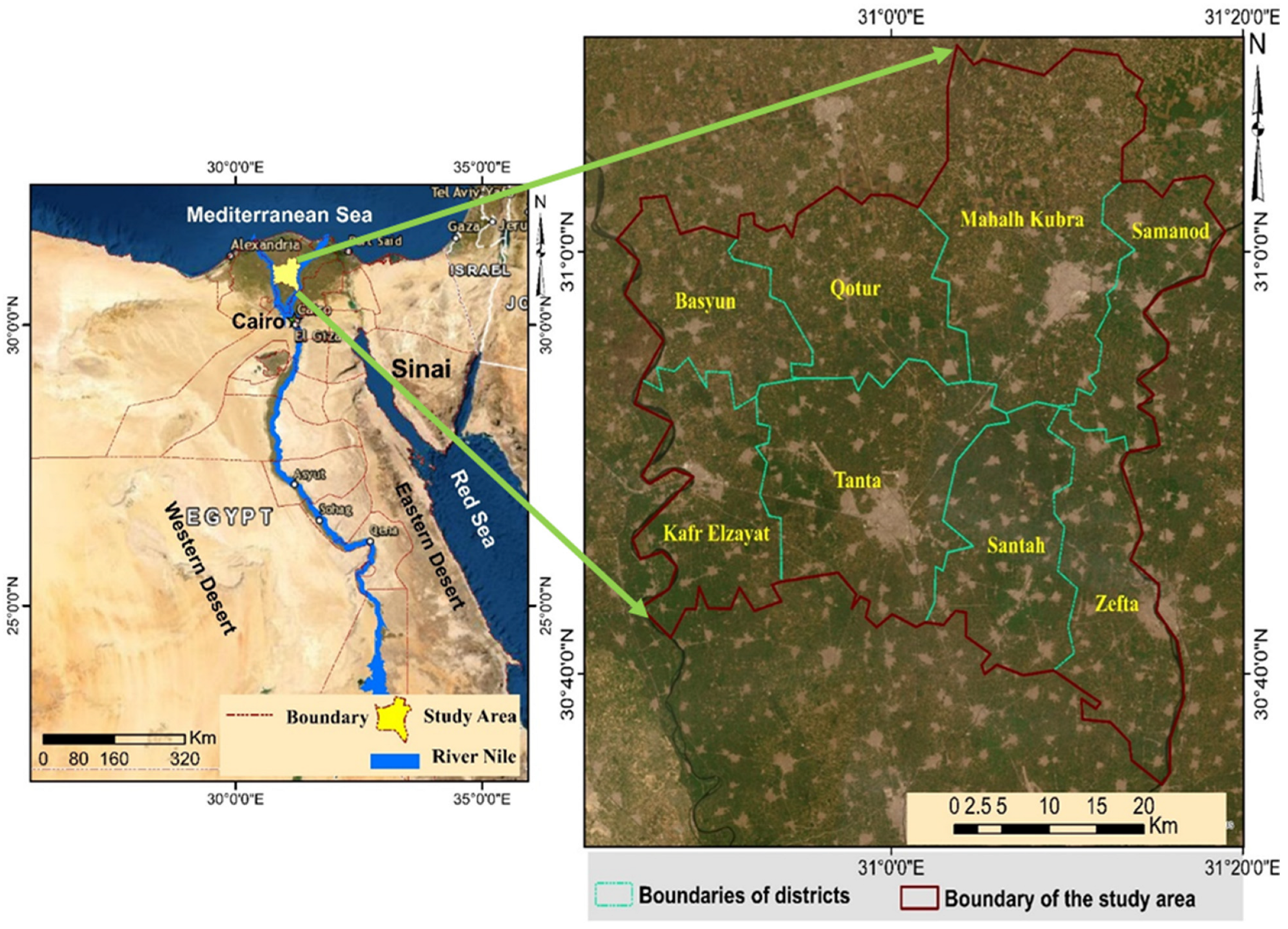
Figure 1. The study area of Gharbia governorate, Egypt [35].
Remotesensing 15 00843 g001
Figure 2. The conceptual flowchart of the adopted methodology. (a) Supervised classification of the processed images for obtaining LULC maps; (b) simulating the LULCC using CA-Markov chain model and the integrated model of CA-Markov chain with FAHP; and (c) estimation of LST and investigating the impact of LULCC on LST based on regression analysis; and (d) conducting regression analysis to obtain the relationship between LULC and the corresponding LST.
Remotesensing 15 00843 g002
Figure 3. Spatial distribution of LULC over the study area during the study period: (a) LULC map in 1991; (b) LULC map in 2003; and (c) LULC map in 2018.
Remotesensing 15 00843 g003
Figure 4. The simulated LULC for 2018 obtained based on the traditional CA-Markov model.
Remotesensing 15 00843 g004
Figure 5. Simulated LULC map for 2018 based on the hybrid model of FAHP-CA-Markov chain.
Remotesensing 15 00843 g005
Figure 6. Projected land cover for 2033 and 2048, respectively.
Remotesensing 15 00843 g006
Figure 7. Spatial distribution of daytime land surface temperature (LST) over the study area during the study period in June 1991, 2003, and 2018, all at around 8:00 am.
Remotesensing 15 00843 g007
Figure 8. Land surface temperature maps illustrating UHI intensity and UHI zones. The white color represents non-UHI zones, and UHI intensity is mentioned for each image.
Remotesensing 15 00843 g008
Figure 9. Regression analysis to retrieve the relationship between the LST and LULC over Gharbia in (a) 1991, (b) 2003, and (c) 2018.
Remotesensing 15 00843 g009
Table 1. Description of data used.
Data TypeCapture DateResolutionSourceOutput
Landsat 1991™27 June 199130 mUSGSLULC map
Landsat 2003™28 June 200330 mUSGSLULC map
Landsat 2018OLI-TIRS21 June 201830 mUSGSLULC map
Google Earth historical imagesJune 1991, 2003, 2018 Google Earth ProTraining/validation
Road network layer OSMDistance to nearest road
Table 2. The fuzzified pairwise comparison matrix of nine criteria selected for the study area.
CriteriaLULCDist. to Persist. Built-UpDist. to Urban CentersDist. to Railway StationsDist. to Near RoadNeighbor. EffectPopulation DensityLocal Develop.Employment
LULC(1,1,1) ( 1 9 , 1 8 , 1 7 ) ( 1 9 , 1 8 , 1 7 ) ( 1 8 , 1 7 , 1 6 ) ( 1 9 , 1 8 , 1 7 ) ( 1 8 , 1 7 , 1 6 ) ( 1 6 , 1 5 , 1 4 ) ( 1 6 , 1 5 , 1 4 ) ( 1 8 , 1 7 , 1 6 )
Dist. to persist. built-up(7,8,9)(1,1,1)(1,1,1)(4,5,6)(2,3,4)(1,1,1)(2,3,4)(2,3,4)(2,3,4)
Dist. to urban centers(7,8,9)(1,1,1)(1,1,1)(2,3,4)(1,2,3)(1,1,1)(2,3,4)(3,4,5)(2,3,4)
Dist. to railway stations(6,7,8) ( 1 6 , 1 5 , 1 4 ) ( 1 4 , 1 3 , 1 2 ) (1,1,1) ( 1 4 , 1 3 , 1 2 ) ( 1 6 , 1 5 , 1 4 ) (1,1,1)(2,3,4)(1,1,1)
Dist. to nearest road(7,8,9) ( 1 4 , 1 3 , 1 2 ) ( 1 3 , 1 2 , 1 ) (2,3,4)(1,1,1) ( 1 4 , 1 3 , 1 2 ) (2,3,4)(3,4,5)(2,3,4)
Neighborhood effect(6,7,8)(1,1,1)(1,1,1)(4,5,6)(2,3,4)(1,1,1)(1,1,1)(2,3,4)(2,3,4)
Population density(4,5,6) ( 1 4 , 1 3 , 1 2 ) ( 1 4 , 1 3 , 1 2 ) (1,1,1) ( 1 4 , 1 3 , 1 2 ) (1,1,1)(1,1,1) ( 1 4 , 1 3 , 1 2 ) (1,1,1)
Local development(4,5,6) ( 1 4 , 1 3 , 1 2 ) ( 1 5 , 1 4 , 1 3 ) ( 1 4 , 1 3 , 1 2 ) ( 1 5 , 1 4 , 1 3 ) ( 1 4 , 1 3 , 1 2 ) (2,3,4)(1,1,1) ( 1 3 , 1 2 , 1 )
Employment(6,7,8) ( 1 4 , 1 3 , 1 2 ) ( 1 4 , 1 3 , 1 2 ) (1,1,1) ( 1 4 , 1 3 , 1 2 ) ( 1 4 , 1 3 , 1 2 ) (1,1,1)(1,2,3)(1,1,1)
Table 3. Classification accuracy assessment of LULC types.
AccuracyLULC Class199120032018
User’s accuracy (%)Built-up80.785.791.8
Water82.182.694.7
Agricultural land97.096.495.1
Producer’s accuracy (%)Built-up80.080.981.3
Water82.186.485.7
Agricultural land97.197.298.1
Overall accuracy (%) 94.994.794.6
Kappa coefficient 0.780.810.84
Table 4. Details of LULCC in the Gharbia governorate in 1991, 2003, and 2018.
LULC199120032018
Area (km2)%Area (km2)%Area (km2)%
Built-up156.757.8193.379.7303.7515.2
Water19.571.024.481.221.561.1
Agricultural land1832.0191.21781.4889.11674.0283.7
Total1999.331001999.331001999.33100
Table 5. Weights of the selected criteria based on AHP and FAHP models.
Model CriteriaAHPFAHP
LULC0.0170
Dist. to persistent built-up area0.2020.260
Dist. to urban centers0.1850.238
Dist. to railway stations0.070.040
Dist. to nearest road0.1340.206
Neighborhood effect0.1860.226
Population density0.0710
Local development0.0650
Employment0.070.030
Table 6. The area predicted for each LULC in the study area in 2033 and 2048.
LULC201820332048RD% 2018–2033RD% 2018–2033
Area (km2)%Area (km2)%Area (km2)%
Built-up251.6212.6414.9020.7514.0025.764.9104.3
Water24.481.221.561.121.561.1−11.9−11.9
Agricultural land1723.2386.21562.8778.21463.7773.2−9.3−15.1
Total1999.331001999.331001999.33100
Table 7. Calculation of urban heat island intensity from land surface temperature (LST) based on Landsat images.
Image Acquisition DateMean Urban LST (°C)Mean Rural LST (°C) UHI (°C)
199132.4829.233.25
200337.2932.574.72
201841.5037.464.04
Table 8. Calculation of UHI intensities from land surface temperature (LST) based on Landsat images.
Urban LST (°C)Rural LST (°C)UHI (°C)
DistrictsMean Temperature (μ) 1991Mean Temperature (μ) 2003Mean Temperature (μ) 2018Mean Temperature (μ) 1991Mean Temperature (μ) 2003Mean Temperature (μ) 2018199120032018
Mahalla Kubra32.1636.6240.6328.6531.0936.263.515.534.37
Tanta32.8737.9541.2929.7733.3037.383.104.653.91
Basyun32.8036.7740.4229.8932.4438.192.914.332.23
Zefta32.3237.8441.5029.2933.8638.263.033.983.24
Santah32.4137.6541.0229.3233.3137.443.094.343.58
Kafr Elzayat32.7438.0341.4029.4334.4439.483.313.591.92
Samanod31.7236.5340.5328.5231.9236.583.24.613.95
Qotur32.7436.7041.0429.4531.7637.773.294.943.27
Disclaimer/Publisher’s Note: The statements, opinions and data contained in all publications are solely those of the individual author(s) and contributor(s) and not of MDPI and/or the editor(s). MDPI and/or the editor(s) disclaim responsibility for any injury to people or property resulting from any ideas, methods, instructions or products referred to in the content.