
Evaluation of Sea Surface Wind Products from Scatterometer Onboard the Chinese HY-2D Satellite


Abstract
:1. Introduction
2. Data and Methods
2.1. ECMWF NWP Data
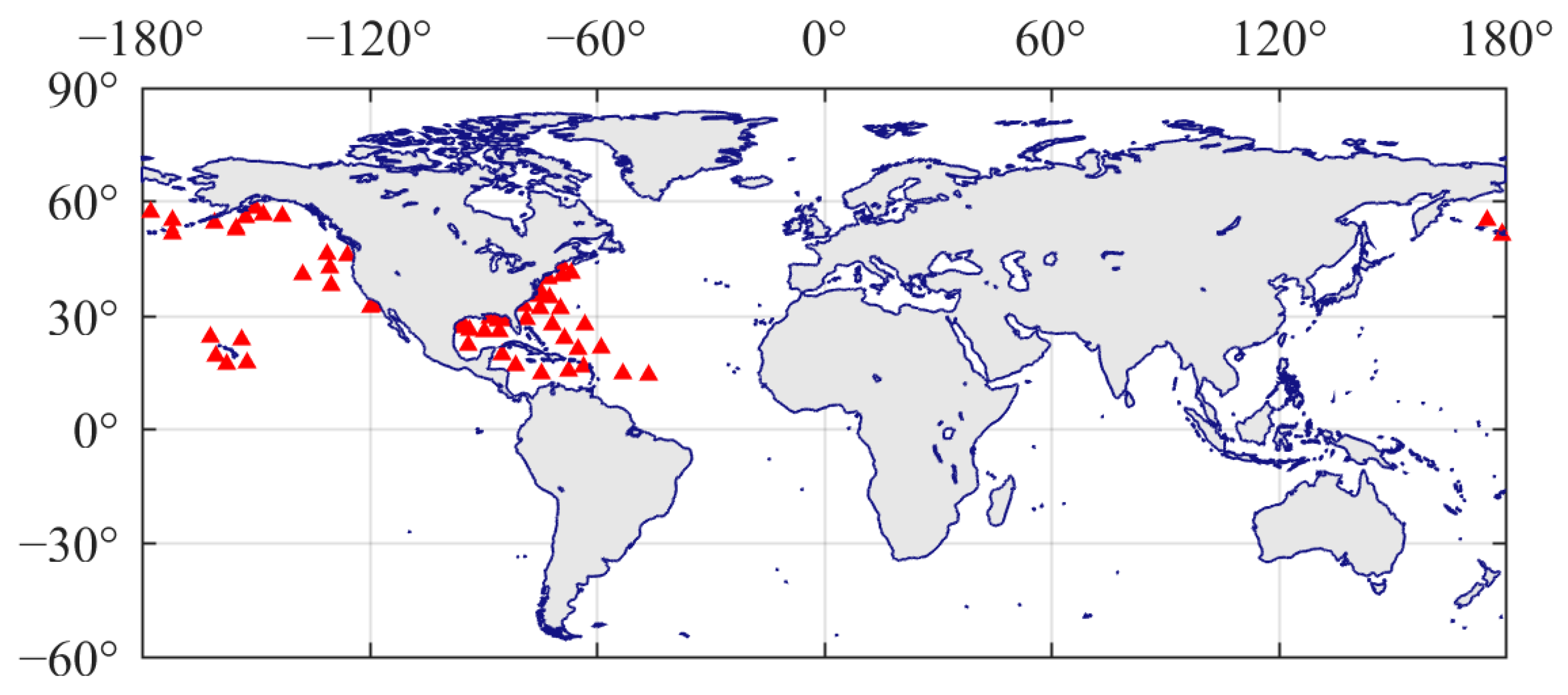
2.2. Buoy Winds
2.3. HSCAT Scatterometer Wind Products
2.4. ASCAT-B Scatterometer Wind Products
2.5. Collocated Datasets
3. Results and Analysis
3.1. Comparision with Buoy Winds
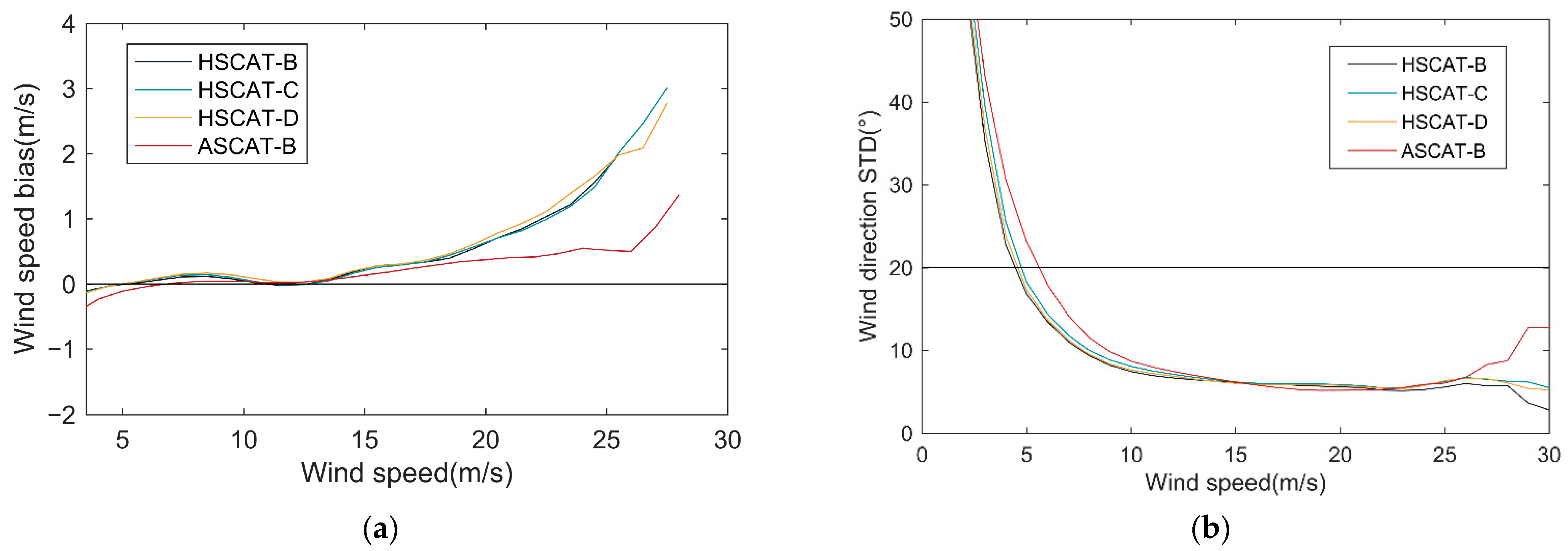
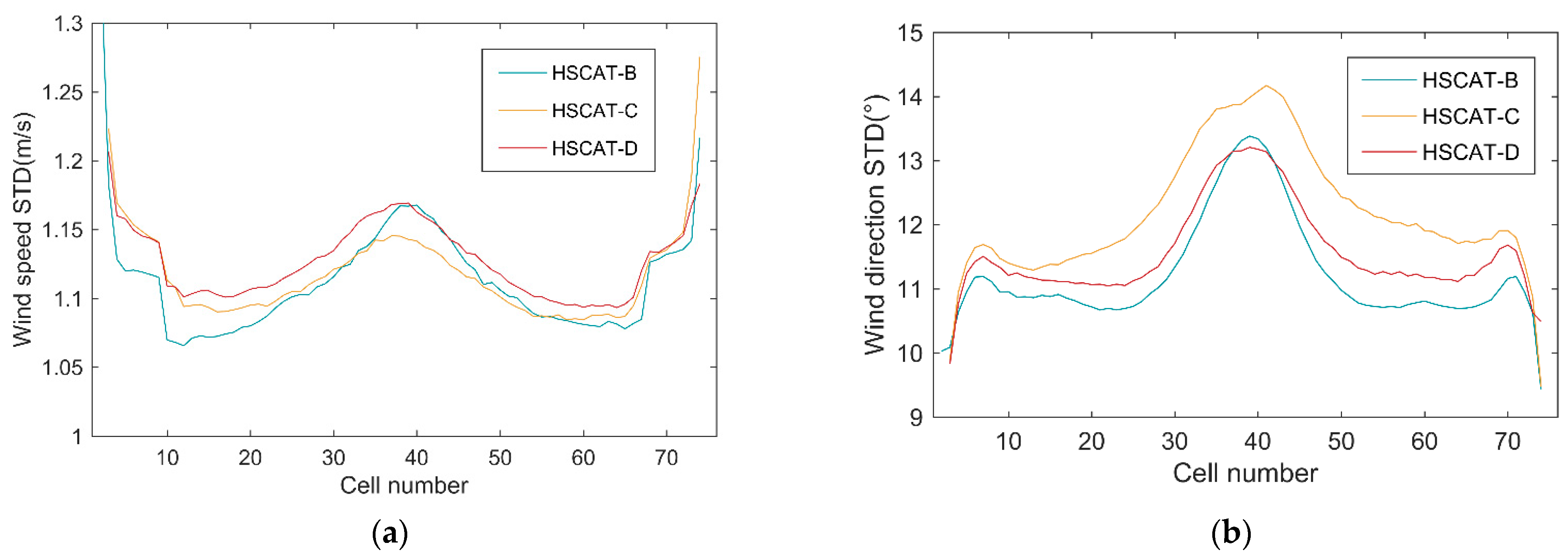
3.2. Comparision with ECMWF Model Winds
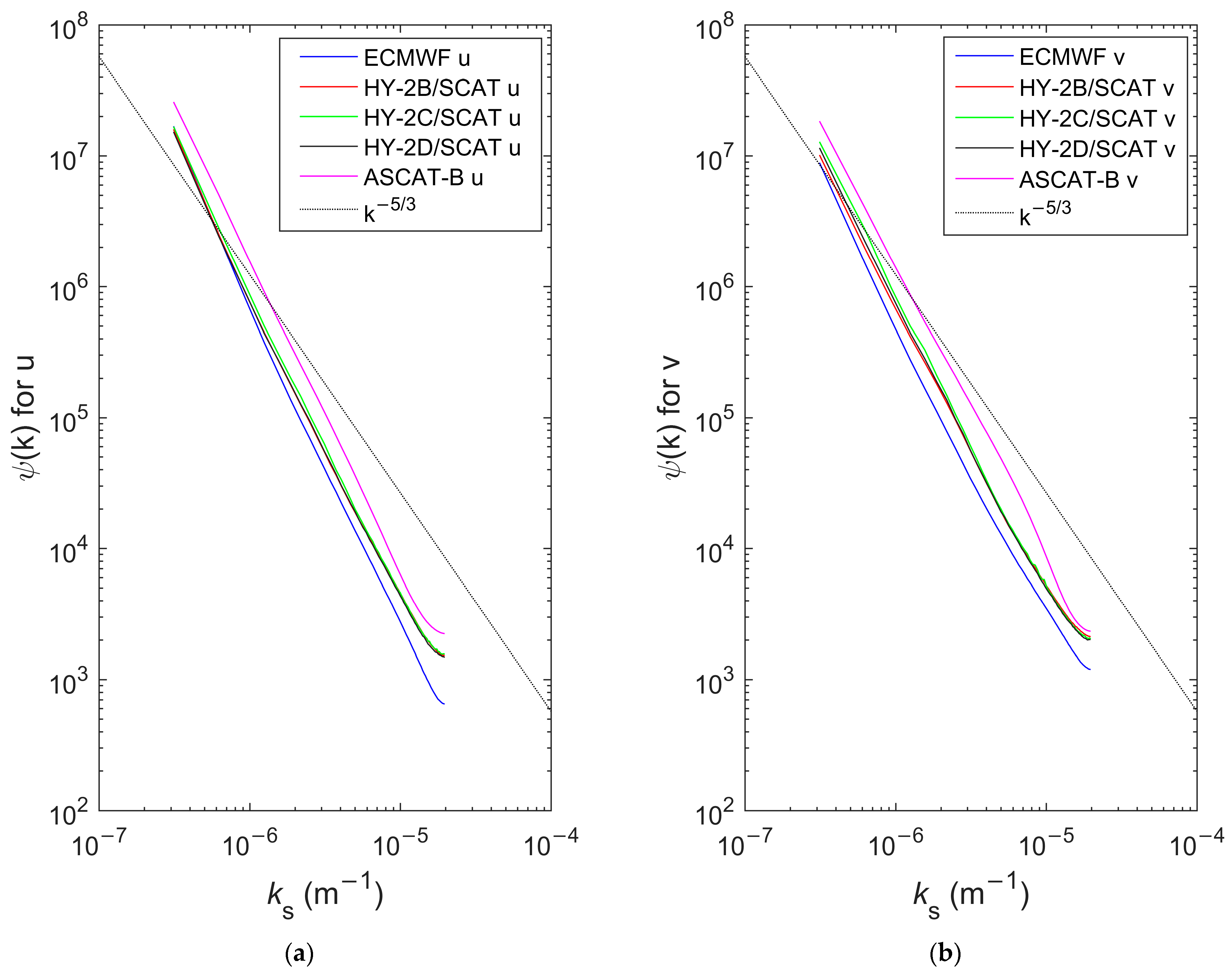
3.3. Spectral Analysis
3.4. Extended Triple Collocation Results
4. Discussion
4.1. Comparison with Other Wind Sources
4.2. Discussion of Spectral and ETC Results
5. Conclusions
Author Contributions
Funding
Data Availability Statement
Conflicts of Interest
References
- Stoffelen, A.; van Beukering, P. The impact of improved scatterometer winds on HIRLAM analyses and forecasts. BCRS Study Contract 1997, 1. [Google Scholar]
- Isaksen, L.; Stoffelen, A. ERS scatterometer wind data impact on ECMWF’s tropical cyclone forecasts. IEEE Trans. Geosci. Remote Sens. 2000, 38, 1885–1892. [Google Scholar] [CrossRef]
- Freilich, M.; Dunbar, R. The accuracy of the NSCAT 1 vector winds comparisons with national data buoy center buoys. J. Geophys. Res. 1999, 104, 11231–11246. [Google Scholar] [CrossRef]
- Bentamy, A.; Croize-Fillon, D.; Perigaud, C. Characterization of ASCAT measurements based on buoy and QuikSCAT wind vector observations. Ocean. Sci. 2008, 4, 265–274. [Google Scholar] [CrossRef]
- Ebuchi, N.; Graber, H.; Caruso, M. Evaluation of wind vectors observed by QuikSCAT/SeaWinds using ocean buoy data. J. Atmos. Ocean. Technol. 2002, 19, 2049–2062. [Google Scholar] [CrossRef]
- Chelton, D.; Freilich, M. Scatterometer-based assessment of 10 m wind analyses from the operational ECMWF and ECMWF numerical weather prediction models. Mon. Weather. Rev. 2005, 133, 409–429. [Google Scholar] [CrossRef]
- Wang, H.; Zhu, J.; Lin, M.; Huang, X.; Zhao, Y.; Chen, C.; Zhang, Y.; Peng, H. First six months quality assessment of HY–2A SCAT wind products using in situ measurements. Acta Oceanol. Sin. 2013, 32, 27–33. [Google Scholar] [CrossRef]
- Mu, B.; Lin, M.; Peng, H.; Song, Q.; Zhou, W. Validation of wind vectors retrieved by the HY–2 microwave scatterometer using ECMWF model data. Eng. Sci. 2014, 16, 39–45. [Google Scholar]
- Zhu, J.; Dong, X.; Yun, R. Calibration and validation of the HY-2 scatterometer backscatter measurements over ocean. In Proceedings of the 2014 IEEE Geoscience and Remote Sensing Symposium, Quebec City, QC, Canada, 13–18 July 2014; pp. 4382–4385. [Google Scholar]
- Wang, Z.; Stoffelen, A.; Zou, J.; Lin, W.; Verhoef, A.; Zhang, Y.; He, Y.; Lin, M. Validation of New Sea Surface Wind Products from Scatterometers Onboard the HY-2B and MetOp-C Satellites. IEEE Trans. Geosci. Remote Sens. 2020, 58, 4387–4394. [Google Scholar] [CrossRef]
- Wang, Z.; Zou, J.; Stoffelen, A.; Lin, W.; Verhoef, A.; Li, X.; He, Y.; Zhang, Y.; Lin, M. Scatterometer Sea Surface Wind Product Validation for HY-2C. IEEE J. Sel. Top. Appl. Earth Obs. Remote Sens. 2021, 14, 6156–6164. [Google Scholar] [CrossRef]
- Vogelzang, J.; Stoffelen, A.; Verhoef, A.; Figurea-Saldaña, J. On the quality of high-resolution scatterometer winds. J. Geophys. Res. Oceans 2011, 116, 1–14. [Google Scholar] [CrossRef]
- Chakraborty, A.; Kumar, R.; Stoffelen, A. Validation of ocean surface winds from the OCEANSAT-2 scatterometer using triple collocation. Remote Sens. Lett. 2013, 4, 85–94. [Google Scholar] [CrossRef]
- Stoffelen, A. Toward the true near-surface wind speed: Error modeling and calibration using triple collocation. J. Geophys. Res. 1998, 103, 7755–7766. [Google Scholar] [CrossRef]
- McColl, K.A.; Vogelzang, J.; Konings, A.G.; Entekhabi, D.; Piles, M.; Stoffelen, A. Extended triple collocation: Estimating errors and correlation coeffients with respect to anunknown target. Geophys. Res. Lett. 2014, 41, 6229–6236. [Google Scholar] [CrossRef]
- Verhoef, A.; Stoffelen, A. Quality Control of Ku-Band Scatterometer Winds; SAF/OSI/CDOP2/KNMI/TEC/RP/194; OSI SAF: De Bilt, The Netherlands, 2012. [Google Scholar]
- de Kloe, J.; Stoffelen, A.; Verhoef, A. Verhoef, Improved Use of Scatterometer Measurements by Using Stress-Equivalent Reference Winds. IEEE J. Sel. Top. Appl. Earth Obs. Remote. Sens. 2017, 10, 2340–2347. [Google Scholar] [CrossRef]
- Liu, W.; Tang, W. Equivalent Neutral Wind; California Institute of Technology: Pasadena, CA, USA, 1996. [Google Scholar]
- National Satellite Ocean Application Service (NSOAS). HY-2B Scatterometer Wind Product User Manual, Version 1.1, 2018, NSOAS. Available online: https://osdds.nsoas.org.cn/ (accessed on 1 December 2022).
- Stoffelen, A.; Portabella, M. On Bayesian scatterometer wind inversion. IEEE Trans. Geosci. Remote Sens. 2006, 44, 1523–1533. [Google Scholar] [CrossRef]
- Wang, Z.; Zhao, C.; Zou, J.; Xie, X.; Zhang, Y.; Lin, M. An improved wind retrieval algorithm for the HY-2A scatterometer. Chin. J. Oceanol. Limnol. 2015, 33, 1201–1209. [Google Scholar] [CrossRef]
- OSI SAF/EARS Winds Team. ASCAT Wind Product User Manual. SAF/OSI/CDOP/KNMI/TEC/MA/126, Version 1.17, OSI SAF. 2021. Available online: https://scatterometer.knmi.nl/publications/pdf/ASCAT_Product_Manual.pdf (accessed on 1 December 2021).
- Stofflen, A. A simple method for calibration of a scatterometer over the ocean. J. Atmos. Ocean. Technol. 1999, 16, 275–281. [Google Scholar] [CrossRef]
- Wang, Z.; Stoffelen, A.; Fois, F.; Verhoef, A.; Zhao, C.; Lin, M.; Chen, G. SST dependence of Ku-and C-band backscatter measurements. IEEE J. Sel. Top. Appl. Earth Obs. Remote Sens. 2017, 10, 2135–2146. [Google Scholar] [CrossRef]


| HSCAT-B | HSCAT-C | HSCAT-D | ASCAT-B | |
|---|---|---|---|---|
| Frequency | 13.256 GHz | 13.256 GHz | 13.256 GHz | 5.255 GHz |
| Polarization mode | HH + VV | HH + VV | HH + VV | VV |
| Spatial resolution | 25 km × 25 km | 25 km × 25 km | 25 km × 25 km | 25 km × 25 km |
| Swath width | 1350 km(H)/1700 km(V) | 1350 km(H)/1700 km(V) | 1350 km(H)/1700 km(V) | 500 km |
| Incidence angles | 48°(V)/41°(H) | 48°(V)/41°(H) | 48°(V)/41°(H) | 25°–65° |
| Antenna | Rotating pencil beam | Rotating pencil beam | Rotating pencil beam | Fan beam |
| Wind speed precision | ±2 m/s or 10% (2~24 m/s) | ±2 m/s or 10% (2~24 m/s) | ±2 m/s or 10% (2~24 m/s) | ±2 m/s or 10% (4~24 m/s) |
| Wind direction precision | ±20° | ±20° | ±20° | ±20° |
| Name | Number | Speed | U | V | Direction | |||
|---|---|---|---|---|---|---|---|---|
| Bias (m/s) | STD (m/s) | Bias (m/s) | STD (m/s) | Bias (m/s) | STD (m/s) | RMSE (°) | ||
| HSCAT-D | 23,229 | −0.03 | 0.78 | −0.01 | 1.18 | −0.01 | 1.23 | 14.10 |
| HSCAT-B | 20,696 | −0.07 | 0.77 | 0.04 | 1.18 | −0.03 | 1.18 | 13.92 |
| HSCAT-C | 23,979 | −0.04 | 0.81 | 0.03 | 1.26 | −0.04 | 1.28 | 15.10 |
| ASCAT-B | 14,573 | −0.01 | 0.77 | 0.04 | 1.08 | 0.09 | 1.24 | 14.97 |
| Name | QC | Speed | U | V | Direction | |||
|---|---|---|---|---|---|---|---|---|
| Bias (m/s) | STD (m/s) | Bias (m/s) | STD (m/s) | Bias (m/s) | STD (m/s) | RMSE (°) | ||
| HSCAT-D | 7.7% | 0.09 | 1.15 | −0.18 | 1.25 | 0.00 | 1.25 | 12.79 |
| HSCAT-B | 6.3% | 0.06 | 1.14 | −0.10 | 1.26 | 0.06 | 1.21 | 12.69 |
| HSCAT-C | 6.5% | 0.07 | 1.14 | −0.16 | 1.29 | 0.00 | 1.27 | 13.51 |
| ASCAT-B | 1.0% | 0.04 | 1.04 | −0.06 | 1.28 | −0.09 | 1.37 | 14.27 |
| NAME | Scatterometer | Buoy | ECMWF | |||
|---|---|---|---|---|---|---|
| εu (m/s) | εv (m/s) | εu (m/s) | εv (m/s) | εu (m/s) | εv (m/s) | |
| HSCAT-B | 0.60 | 0.46 | 1.02 | 1.08 | 0.98 | 1.00 |
| HSCAT-C | 0.71 | 0.63 | 1.04 | 1.11 | 0.97 | 0.96 |
| HSCAT-D | 0.61 | 0.57 | 1.00 | 1.09 | 0.97 | 0.96 |
| ASCAT-B | 0.39 | 0.54 | 1.00 | 1.11 | 1.16 | 1.20 |
| NAME | Scatterometer | Buoy | ECMWF | |||
|---|---|---|---|---|---|---|
| HSCAT-B | 0.995 | 0.996 | 0.985 | 0.978 | 0.987 | 0.981 |
| HSCAT-C | 0.993 | 0.993 | 0.985 | 0.977 | 0.988 | 0.982 |
| HSCAT-D | 0.995 | 0.994 | 0.986 | 0.978 | 0.987 | 0.982 |
| ASCAT-B | 0.998 | 0.995 | 0.986 | 0.978 | 0.982 | 0.973 |
| Name | (m/s) | (m/s) | ||
|---|---|---|---|---|
| HSCAT-B | 1.003 | 0.986 | 0.057 | 0.104 |
| HSCAT-C | 0.994 | 0.987 | 0.064 | 0.096 |
| HSCAT-D | 0.993 | 0.984 | 0.091 | 0.061 |
| ASCAT-B | 0.983 | 0.981 | 0.013 | −0.035 |
Disclaimer/Publisher’s Note: The statements, opinions and data contained in all publications are solely those of the individual author(s) and contributor(s) and not of MDPI and/or the editor(s). MDPI and/or the editor(s) disclaim responsibility for any injury to people or property resulting from any ideas, methods, instructions or products referred to in the content. |
© 2023 by the authors. Licensee MDPI, Basel, Switzerland. This article is an open access article distributed under the terms and conditions of the Creative Commons Attribution (CC BY) license (https://creativecommons.org/licenses/by/4.0/).
Share and Cite
Yang, S.; Zhang, L.; Lin, M.; Zou, J.; Mu, B.; Peng, H. Evaluation of Sea Surface Wind Products from Scatterometer Onboard the Chinese HY-2D Satellite. Remote Sens. 2023, 15, 852. https://doi.org/10.3390/rs15030852
Yang S, Zhang L, Lin M, Zou J, Mu B, Peng H. Evaluation of Sea Surface Wind Products from Scatterometer Onboard the Chinese HY-2D Satellite. Remote Sensing. 2023; 15(3):852. https://doi.org/10.3390/rs15030852
Chicago/Turabian StyleYang, Sheng, Lu Zhang, Mingsen Lin, Juhong Zou, Bo Mu, and Hailong Peng. 2023. "Evaluation of Sea Surface Wind Products from Scatterometer Onboard the Chinese HY-2D Satellite" Remote Sensing 15, no. 3: 852. https://doi.org/10.3390/rs15030852
APA StyleYang, S., Zhang, L., Lin, M., Zou, J., Mu, B., & Peng, H. (2023). Evaluation of Sea Surface Wind Products from Scatterometer Onboard the Chinese HY-2D Satellite. Remote Sensing, 15(3), 852. https://doi.org/10.3390/rs15030852