ANLPT: Self-Adaptive and Non-Local Patch-Tensor Model for Infrared Small Target Detection

Abstract

Infrared small target detection is widely used for early warning, aircraft monitoring, ship monitoring, and so on, which requires the small target and its background to be represented and modeled effectively to achieve their complete separation. Low-rank sparse decomposition based on the structural features of infrared images has attracted much attention among many algorithms because of its good interpretability. Based on our study, we found some shortcomings in existing baseline methods, such as redundancy of constructing tensors and fixed compromising factors. A self-adaptive low-rank sparse tensor decomposition model for infrared dim small target detection is proposed in this paper. In this model, the entropy of image block is used for fast matching of non-local similar blocks to construct a better sparse tensor for small targets. An adaptive strategy of low-rank sparse tensor decomposition is proposed for different background environments, which adaptively determines the weight coefficient to achieve effective separation of background and small targets in different background environments. Tensor robust principal component analysis (TRPCA) was applied to achieve low-rank sparse tensor decomposition to reconstruct small targets and their backgrounds separately. Sufficient experiments on the various types data sets show that the proposed method is competitive.

1. Introduction

Due to the advantages of all-weather, long-distance observation, infrared imaging technology is widely used in military and civilian fields, such as target searching, early warning and tracking [1,2,3]. The targeted observation based on infrared imaging has the characteristics of small size and weak signal intensity (for an image size of $256\times 256$, the widely recognized small target should be less than $9\times 9$ pixel) [4]. At the same time, thermal infrared imaging is the sensor’s perception of the thermal radiation of the target, so the resolution of the image is low. The inherent difficulty of infrared small target detection and its wide application value make it a hotspot of current research. However, due to the small target scale and low resolution, the small targets in thermal infrared imaging almost lack textural features and clear contour features and only show dim and small bright spots in the image. Effectively extracting small infrared targets in a complex background with clutters is still full of challenges and many key problems need to be solved.

Infrared dim and small target detection methods are generally divided into detection based on single-frame images and detection based on multi-frame images. Infrared dim and small target detection methods based on multiple frames often need the movement information of targets in sequences, such as 3D matched filtering [5], TLPP [6], IVERS [7], TCTHR [8], SCTP [9]. However, in practical application scenarios, the following scenarios may even exist simultaneously: (1) The observed target is moving fast; (2) Clouds and geothermal noise in the background also move rapidly; (3) The load platform of the sensor moves at high speed. Therefore, the performance of the infrared dim small target detection method based on multi-frames will be greatly affected when the background is not fixed. Meanwhile, computational efficiency and other factors also limit the application of this method. Therefore, small dim target detection methods based on a single frame have more universal application scenarios and need to be further studied. This paper focuses on dim and small target detection based on one single-frame image.

The target in the infrared image generally has a higher brightness than the surrounding environment, and is showing a small but bright spot. Based on this intuitive clue, a variety of representative methods have been proposed, such as Max-Mean and Max-Median filters [10], the Top-Hat filter and its improvement [11,12]. Based on least mean square (LMS), Hadhoud and Thomas [13] proposed a two-dimensional LMS (2DLMS) filter and improved it for the detection of infrared small targets [14,15]. Some morphology-based methods [16,17,18,19,20] also make use of this idea. However, these methods are often based on the assumption that the background is viewed as continuous and that the target brightness is greater than all backgrounds. Therefore, when the image has clutter and noise, the detection performance of this method decreases significantly.

Based on the mechanism of observing objects in human vision, a variety of object detection methods based on the human vision system (HVS) have been proposed. These object detection methods use three HVS mechanisms [21], namely the contrast mechanism, visual attention, and eye movement to find targets that meet the characteristics of these mechanisms. Chen et al. [4] designed and proposed a multi-scale infrared small target detection method (LCM) based on the HVS and DK (derived kernel) model, as well as the discontinuity between small targets and their neighborhoods. On this basis, researchers have improved and proposed a variety of novel methods based on local contrast. For example, Qin and Li [22] proposed a novel local comparison method NLCM; Han et al. [23] proposed the multi-scale correlation local comparison method MRLCM; Liu et al. [24] proposed the weight local comparison method WLCM. The three-layer local contrast method (TLLCM) proposed by Han et al. [25] enhances the target of the image before local comparison and divides the comparison window into a core layer, reverse layer, and surrounding layer to calculate the comprehensive contrast. However, discontinuities exist not only between targets and their backgrounds but also between some brighter clutters and their backgrounds. Therefore, these kinds of methods cannot distinguish clutter noises and targets effectively.

Deep learning can be used to learn the features of small targets [26,27]. One kind of method is to use a deep neural network for small target segmentation based on the idea of image segmentation [28,29]. Another kind of method based on the idea of image recognition is to use a deep neural network for target and background recognition [27,30]. Existing studies have shown that deep learning still difficult to represent and learn the features of weak and small targets, and the model is easy to overfit and other obstacles. Especially in the case of fewer target pixels, complex target distribution, and background mode, the detection performance is degraded due to the huge sample space [31,32]. Moreover, such methods usually require a large amount of training data, which is difficult to obtain in practical applications. In addition, the unexplainability of deep neural networks also hinders their application in the field of high reliability.

After analyzing the structure of the infrared small target and the image background, researchers find that the small target in the infrared image is sparse both in the global image and in a local area with appropriate size. Moreover, the background is considered low-rank in the infrared image [2]. Therefore, by establishing an appropriate low-rank and sparse decomposition model, the background part (low-rank component) and the target part (sparse component) of the infrared image can be effectively separated to detect dim small targets. The infrared patch-image (IPI) model proposed by Gao et al. [2] constructs the original data matrix of the local image block by sliding the window on the image according to the given step and then solves this prototype through the RPCA pair optimization to realize the detection of sparse targets in it. Inspired by the IPI method, various models for the decomposition of low-rank sparse matrices have been proposed. Dai et al. [33] provides a weighted infrared patch-image (WIPI) model by taking the local structure of the image as prior information and integrating it into decomposition. Wang et al. [34] proposed a PILGA model combining local and global information of infrared images. The target-aware non-local low-rank modeling with saliency filtering proposed by Zhu et al. [35] regularization takes into account the non-local sparsity of the infrared image and increases the anti-interference ability of the model by saliency filtering regularization.

However, the real-time performance of PI-based models is often poor, and it is difficult to extract the 2D local environment information of pixels. A patch-tensor (PT) model has been proposed, based on the idea of PI and featuring tensor data in much higher dimensions (usually three dimensions). Among them, the reweighted infrared patch-tensor (RIPT) proposed by Dai and Wu [36] is a kind of model combining local and non-local prior information of images. In 2020, Zhang et al. [37] proposed the partial sum of the tensor nuclear norm (PSTNN) model by analyzing the rank of tensor. In 2021, Kong et al. [38] used the rank of the tensor to derive the tensor fiber rank, and calculated the tensor fiber rank approximately by the log operator. Then, a nonconvex tensor fibered rank approximation (NTFRA) method was proposed for infrared small target detection.

Both PI and PT based methods use a sliding window to traverse the entire image. The difference is that the PI-based model converts each obtained patch image into a vector and combines all the vectors to get a large matrix, while the PT model uses each patch image as a frontal slice and constructs a large tensor. There are some defects in their practical application as follows: (1) For images with complex backgrounds, the prototype data (matrix or tensor) constructed by this global mode have weak low-rank sparsity, which makes decomposition difficult; (2) The compromising factor used to fix low-rank and sparse parts decreases performance in globally inconsistent backgrounds; (3) The decomposition of a large original data structure is time-consuming and cannot be parallelized.

A segmented adaptive non-local patch-tensor model for infrared small target detection is proposed. It constructs a small tensor for each reference block in the image through non-local block matching and separates the background and target foreground by low-rank sparse decomposition of the small tensor. The proposed method has the following obvious advantages: (1) Image local entropy is used to realize the non-local MDB matching of image blocks, and build a small tensor with better low-rank sparse characteristics. The size of the tensor is $n_1\times n_2\times (t+1)$, where $n_1$ and $n_2$ indicate the size of the image block. However, t is a very small value, and it is found in the experiment that when its value is set to 2, the model has a good performance; (2) It can adaptively select a low-rank sparse compromising factor according to the distribution of different backgrounds of image blocks, so that the model has a better effect of background target separation; (3) Our method can divide the image with length W and width H into $WH/n_1{n}_2$ unrelated construction tasks and optimization tasks in parallel, so it has the advantage of fast computation. The extraction effect of our method on small and weak target regions is shown in Figure 1.

The main contributions of this paper are as follows:

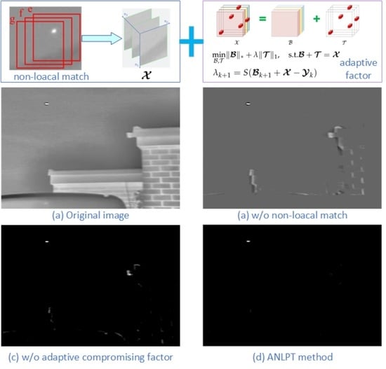
• An adaptive non-local patch-tensor model for infrared small target detection is proposed. By combining the background consistency and local similarity, the image local entropy was used to construct a non-local block tensor with good low-rank sparse characteristics for image blocks. Then, the proposed adaptive compromising factor and TRPCA were used to achieve the effective separation of background and small target;
• The mapping relationship between image local entropy and compromising factor was explored, and a dynamic and adaptive compromising factor is proposed for an effectively low-rank and sparse decomposition strategy. Our approach has a better performance when the background is not globally consistent;
• Experiments on various data sets with different characteristics show that the proposed method is more competitive than the state-of-the-art methods.

The structure of this paper is as follows: Section 2 states the various notation definitions used in this article. Section 3 describes the proposed method in detail. Section 4 introduces the comparison experiment and evaluation standard. Section 5 summarizes the proposed method.

2. Notations and Fundamentals

In this paper, scalars are represented by plain lowercase letters, e.g., a. Vectors are represented by bold lowercase letters, e.g., $\mathit{v}$. Matrices are represented by bold uppercase letters, e.g., $\mathit{M}$. Tensors are represented by bold Euler capital letters, e.g., $𝓐$. $𝓐(i,j,:)$ is the tube fiber of the ith row and jth column of the tensor $𝓐$, and the ${\mathit{A}}_{\left(i\right)}$ is the ith frontal slice of the tensor $𝓐(:,:,i)$.

2.1. Tensor Singular Value Decomposition(t-SVD)

t-SVD [39] plays an important role in the low-rank and sparse decomposition of tensors. A tensor $𝓐\in {\mathbb{R}}^{n_1\times n_2\times n_3}$ can be decomposed into the product of two orthogonal tensors $𝓤\in {\mathbb{R}}^{n_1\times n_2\times n_3}$, $𝓥\in {\mathbb{R}}^{n_1\times n_2\times n_3}$ and f-diagonal tensor $𝓢\in {\mathbb{R}}^{n_1\times n_2\times n_3}$ by t-SVD as:

$$𝓐=𝓤\ast 𝓢\ast {𝓥}^{*}.$$

(1)

Algorithm 1 shows the detailed process of t-SVD.

For the t-SVD of a real tensor $𝓐$ with size $n_1\times n_2\times n_3$, each tube fiber is transformed by a fast Fourier transform (FFT) to obtain the corresponding tensor $𝓓$. Then, each of the frontal slices ${\mathit{D}}_{\left(i\right)}$, ${\mathit{U}}_{\left(i\right)}$, ${\mathit{S}}_{\left(i\right)}$ and ${\mathit{V}}_{\left(i\right)}$ are obtained by the decomposition of the singular values of the matrix. Next, three tensor $\overline{𝓤}$, $\overline{𝓢}$ and $\overline{𝓥}$ are composed by the index i. Finally, the tensors $𝓤$, $𝓢$ and $𝓥$ are obtained by performing an inverse FFT on each tube fiber of each tensor.

Algorithm 1: t-SVD.

Input: $𝓐\in {\mathbb{R}}^{n_1\times n_2\times n_3}$

foreach tube in $𝓐$do

$\hspace{1em} 𝓓(i,j,:)=\mathrm{fft}(𝓐(i,j,:\left)\right)$;

for$i=1:⌊\frac{n_3+1}{2}⌋$do

$\hspace{1em}[{\overline{\mathit{U}}}_{\left(i\right)},{\overline{\mathit{S}}}_{\left(i\right)},{\overline{\mathit{V}}}_{\left(i\right)}]=\mathrm{svd}\left({\mathit{D}}_{\left(i\right)}\right)$;

for$i=⌊\frac{n_3+1}{2}⌋+1:n_3$do

$\hspace{1em}{\overline{\mathit{U}}}_{\left(i\right)}=\mathrm{conj}\left({\overline{\mathit{U}}}_{(n_3-i+2)}\right)$;

/*conj is conjugate-even vector [40]*/

$\hspace{1em}{\overline{\mathit{S}}}_{\left(i\right)}=\mathrm{conj}\left({\overline{\mathit{S}}}_{(n_3-i+2)}\right)$;

$\hspace{1em}{\overline{\mathit{V}}}_{\left(i\right)}=\mathrm{conj}\left({\overline{\mathit{V}}}_{(n_3-i+2)}\right)$;

foreach tube in $\overline{𝓤}$, $\overline{𝓢}$ and $\overline{𝓥}$do

$\hspace{1em}𝓤(i,j,:)=\mathrm{ifft}\left(\overline{𝓤}(i,j,:)\right)$;

$\hspace{1em}𝓢(i,j,:)=\mathrm{ifft}\left(\overline{𝓢}(i,j,:)\right)$;

$\hspace{1em}𝓥(i,j,:)=\mathrm{ifft}\left(\overline{𝓥}(i,j,:)\right)$;

Output: $𝓤$, $𝓢$, $𝓥$

2.2. The Local Information Entropy of the Image

Information entropy reflects the richness of the information contained in an information source. In an image, the information entropy is defined as:

$$\begin{array}{cc}\hfill E\left(I\right)& =-\sum _{i=0}^{255}p\left(i\right){log}_{2}p\left(i\right),\hfill \end{array}$$

(2)

$$\begin{array}{cc}\hfill p\left(i\right)& =m_i/M_I,\hfill \end{array}$$

(3)

where I is the input image, $m_i$ is the number of pixels of the ith gray value, and $M_I$ is the total number of the patch pixels. If the input is a patch of an image, the image entropy is the part information entropy of the image—called the local entropy of the image—which can reflect the complexity of the image in this area. This property can be used to distinguish local images in infrared images. Figure 2 shows the local entropy feature map (right) of an infrared image (left) with sea-sky edge information. In the feature map, brighter areas indicate higher entropy. Moreover, due to the feature of local similarity in the image, blocks with similar entropy within a certain region tend to have similar structures.

3. The Proposed Algorithm

3.1. The Model Used for Low-Rank Sparse Decomposition of Tensors

An infrared image X composed of background B and target T can be defined as:

$$\mathit{X}=\mathit{B}+\mathit{T}.$$

(4)

We construct a small tensor for each image patch as follows:

$$𝓧=𝓑+𝓣,$$

(5)

where $𝓧$ is the three-dimensional tensor corresponding to a block in the infrared image X, which is built through non-local block matching based on the image’s local entropy. $𝓑$ and $𝓣$ are three-dimensional tensors made up of the background B and the target T in each image block, respectively. Figure 3 shows the structure of the tensor $𝓧$. Suppose that the original tensor consists of a reference image block and two non-local matching blocks, represented in the figure as outer squares with different colors. Each image block acts as a frontal slice of the tensor and may have some information about the targets (red squares in the figure).

The background of an image often changes slowly and multiple local images of an image are always similar, so the background tensor is low rank. Through singular value decomposition of background image blocks, Figure 4 can be obtained. The first row in the figure contains three image blocks selected globally in the image, and the second row contains three image blocks extracted from the image with clear edge information. Figure 4b–d show the results obtained after singular value decomposition of corresponding color blocks in the image respectively. It can be seen that the singular value of the image block, whether global or local, will rapidly decrease to 0. Therefore, each image block has low rank, and the singular values between similar-matched image blocks are more similar.

The rank of the frontal slice of each background tensor is defined as:

$$\mathrm{rank}\left({\mathit{B}}_{\left(i\right)}\right)\le r_i,$$

(6)

where $B_i$ is the ith frontal slice of the background tensor, $r_i$ is a scalar representing the complexity of the corresponding frontal slice. The more complex or informative an image block is, the larger the value of $r_i$.

It is known that the information of small infrared targets in sufficiently large image blocks is always sparse. Using the 0 norm of the tensor, the sparsity of the target is defined as:

$${\parallel 𝓣\parallel }_0\le k,$$

(7)

where k is a sufficiently small integer that satisfies the definition of a sparse tensor. Therefore, the decomposition model of low-rank sparse tensor of infrared small target image under ideal conditions can be defined as:

$$\underset{𝓑,𝓣}{min}\mathrm{rank}(𝓑)+\lambda {\parallel 𝓣\parallel }_0,\mathrm{s}.\mathrm{t}.𝓑+𝓣=𝓧.$$

(8)

3.2. Image Block Matching Based on Local Entropy

To construct a patch tensor with better low-rank sparse characteristics, this paper proposes a non-local image block matching method based on image local entropy. For the low-rank sparse decomposition model (Figure 3), the ideal patch tensor construction method needs to consider two requirements: (1) Whether the method of composing data can meet the requirements of low-rank sparsity; (2) Whether the method of composing data can reasonably retain the small target information in the image. For requirement (1), a direct idea is to implement the block matching strategy by setting reference blocks in the infrared image to find similar non-local matching blocks and form original data structure. The purpose of the non-local block matching method is to find the most similar image blocks with reference blocks in one or more images for image denoising, restoration, or target tracking [41,42,43]. By setting a proper minimum block distortion (MBD), a similar background block can be found in an infrared image to form the original data structure with low-rank property. To achieve the desired result, the corresponding MBD in the common block matching strategy is usually pixel oriented. An infrared small target makes it difficult for these matching strategies to obtain similar background regions. Moreover, the ideal matching mechanism should ignore the influence of existing targets. The image block matching method based on local entropy in this paper can effectively solve this problem. Because the local entropy is an overall statistic of the image block, it is not sensitive to the small dim target region, which occupies a relatively small proportion of the whole image. Moreover, in MBD matching, the local similarity of the image and the continuous consistency of the background are utilized to match image blocks with similar background structures.

Figure 5 shows the results of a block-matching method based on local entropy in an infrared image with rich edge information. In Figure 5a, the block numbered 1 is the reference block. Block matching based on different reference blocks is marked with different colors, and the matching results of blocks numbered 2 and 3 are obtained, respectively. Figure 5b–d show the pixel value-based 3D model of the matching results for the red reference block in Figure 5a; Figure 5e–g show the pixel value-based 3D model of the matching results for the green reference block. It can be seen that the block matching algorithm which takes the local entropy of the image as the MBD retains the structural features of the reference image block itself. Moreover, it can be seen from Figure 5b–g that the image local information entropy matching makes the target and edge position in the matched block independent, which further ensures the constructed tensor more low-rank sparse.

3.3. Adaptive Dynamic Compromising Factor $\lambda$

When baseline methods [2,36,38,44] use low-rank sparse decomposition, the compromising factor on low-rank and sparse parts in Equation (8) is always set to a fixed value:

$$\lambda =\frac{1}{\sqrt{max(n_1,n_2)\times n_3}}.$$

(9)

Based on these works, we find that the size of $\lambda$ directly affects the performance and time consumption of low-rank sparse decomposition. The universal conclusion is: (1) Larger $\lambda$ makes more iterations and time consuming; (2) When $\lambda$ is large, fewer components are retained in the sparse part, and the false alarm is lower when used for dim small target detection. Based on this, an intuitive idea is that, for images with complex backgrounds, a larger compromising factor value can better suppress the interference of background noise. On the contrary, for images with a relatively simple background, a smaller compromising factor can prevent the loss of dim targets and reduce the time consumption of the algorithm. The adaptive dynamic balance factor algorithm is proposed in this paper, which can quantify the complexity of the image background based on the image’s local information entropy and dynamically select the compromising factor $\lambda$ adaptively.

We performed experimental statistical analysis on a large data set. The following laws were found: (1) The range of information entropy of image block applicable to dim small target detection is $e\in [0,8]$; (2) For the tensor decomposition of different backgrounds, the value range of the compromising factor is between $[0,3]$; (3) The compromising factor increases with the increase of the local entropy of the image. Meanwhile, the relationship between the compromising factor and the entropy of the image block with low information is close to linear. In the image block with a complex background, the compromising factor increases more slowly than the entropy value. A modified sigmoid function namely an adaptive compromising factor is proposed to fit the mapping between the compromising factor and entropy, which can be calculated by the following:

$$\begin{array}{cc}\hfill \lambda & =S(\mathbf{ß})=\frac{\alpha \left(\mathrm{sigmoid}\right(M(ß)/\epsilon )-\delta )}{\sqrt{max(n_1,n_2)\times n_3}}\hfill \end{array}$$

(10)

$$\begin{array}{cc}\hfill M(ß)& =\frac{1}{n}\sum _{i=0}^{n}E\left({ß}_{\left(i\right)}\right),\hfill \end{array}$$

(11)

where $M(ß)$ is the average value of entropy calculated by the Equation (2) for each frontal slice in the tensor $ß$ and $\epsilon$, $\delta$ are the scaling and shifting of the $\mathrm{sigmoid}($) function to the independent variable $\overline{e}$, respectively; $\alpha$ is the scaling of the function on the dependent variable to match its desired range of values. In this paper, $\epsilon$, $\delta$, and $\alpha$ are valued as $2.5$, $0.4$, and 5, respectively.

3.4. Adaptive Low-Rank and Sparse Tensor Decomposition Model

The original tensor data shown in Figure 6 can be obtained from Figure 5 using the method described in the previous section, where Figure 6a shows the data with the target, Figure 6b shows the data without the target. For data with target information, a further approximation is needed to obtain the tensor model defined by the Equation (5).

3.4.1. Sparse Approximated Represented of Target by $l_1$-Norm

The $l_0-\mathrm{norm}$ used to calculate the number of non-zero elements in the tensor is a direct representation of the sparsity of the tensor. However, the optimization of $l_0-\mathrm{norm}$ is an NP-hard problem. In practice, $l_1-\mathrm{norm}$ (${\parallel ·\parallel }_1={\sum }_{ij}\left|X_{ij}\right|$) is often used to approximate the sparsity of a pair of tensors. The approximation of $l_0-\mathrm{norm}$ by $l_1-\mathrm{norm}$ can ensure the solution of the model, and also ensure the convex property of the model.

3.4.2. Low-Rank Background Represented by Tensor Nuclear Norm

The nuclear norm is often used as an approximation of the rank of a matrix in low-rank factorization. Extending this knowledge to tensors, a low-rank background was presented in [44] by defining the nuclear norm of the tensor. Before describing the nuclear norm of tensors, there are a few more definitions of tensors that need to be clarified.

Definition 1.

(Tensor tubal rank [45]). For a tensor $𝓐\in {\mathbb{R}}^{n_1\times n_2\times n_3}$, the rank of its tube fibers is the number of non-$\mathbf{0}$ tube fibers in the singular value tensor $𝓢$ in $𝓐=𝓤\ast 𝓢\ast {𝓥}^{*}$ decomposed by t-SVD, that is,

$${\mathrm{rank}}_t(𝓐)=\#\{i,𝓢(i,i,:)\ne \mathbf{0}\}.$$

(12)

Definition 2.

(Tensor average rank). For a tensor $𝓐\in {\mathbb{R}}^{n_1\times n_2\times n_3}$, its average rank is the ratio of the rank of its cyclic block matrix to the number of plane slices, i.e.,

$${\mathrm{rank}}_a(𝓐)=\frac{1}{n_3}rank\left(circ\left(unfold(𝓐)\right)\right).$$

(13)

There is a certain relationship between the rank of the tube fiber and the average rank of the tensor. This relation is that if the block diagonal matrix of the tensor $𝓐$ is $\overline{𝓐}$, then the rank of the tensor’s tube fiber and its average rank are as follows:

$$\begin{array}{cc}\hfill {\mathrm{rank}}_a(𝓐)& =\frac{1}{n_3}\mathrm{rank}\left(\overline{\mathit{A}}\right)\hfill \\ \hfill & \le \underset{i=n_1,\cdots ,n_3}{max}\mathrm{rank}\left({\overline{\mathit{A}}}_{\left(i\right)}\right)\hfill \\ \hfill & ={\mathrm{rank}}_t(𝓐).\hfill \end{array}$$

(14)

This is also the reason why the nuclear norm of the tensor is defined as a convex hull of the average rank of the tensor. After the definition of the tensor tubal rank and the average rank of the tensor, the nuclear norm of the tensor can be defined.

Definition 3.

(Tensor nuclear norm [44]). Let $𝓐=𝓤\ast 𝓢\ast {𝓥}^{*}$ be t-SVD of tensor $𝓐\in {\mathbb{R}}^{n_1\times n_2\times n_3}$, then its nuclearnorm ${\parallel ·\parallel }_{*}$ is defined as:

$${\parallel 𝓐\parallel }_{*}:=\langle 𝓢,𝓘\rangle =\sum _{i=1}^r𝓢(i,i,1),$$

(15)

where rrepresents the tubular fiber rank ${rank}_t(𝓐)$ of the tensor.

The nuclear norm of the tensor $𝓐$ is actually the matrix nuclear norm of its t-SVD slice ${\mathit{A}}_{\left(1\right)}$ on its first side. In t-SVD, the singular value tensor can be obtained by the FFT, so:

$${\parallel 𝓐\parallel }_{*}=\frac{1}{n_3}{\parallel \mathrm{circ}\left(\mathrm{unfold}(𝓐)\right)\parallel }_{*}=\frac{1}{n_3}{\parallel \overline{\mathit{A}}\parallel }_{*}.$$

(16)

From the above equations and the relation in Equation (14), it is clear that the nuclear norm of the tensor defined in Definition 3 is indeed a convex hull of the mean rank of the tensor. Therefore, according to the low-rank sparse decomposition model shown in the Equation (5), the low-rank sparse decomposition model proposed in this paper can be solved as follows:

$$\begin{array}{cc}\hfill & \underset{𝓑,𝓣}{min}{\parallel 𝓑\parallel }_{*}+\lambda {\parallel 𝓣\parallel }_1,\mathrm{s}.\mathrm{t}.𝓑+𝓣=𝓧\hfill \\ \hfill & \lambda =S(\mathbf{ß}).\hfill \end{array}$$

(17)

3.5. Alternating Direction Method of Multiplier (ADMM)

The low-rank sparse decomposition model of tensors based on t-SVD can be optimized by ADMM to solve [44]. Based on the low-rank sparse model mentioned in the previous section, an augmented Lagrangian function based on (17) is constructed, which is:

$$\begin{array}{cc}\hfill L(𝓑,𝓣,𝓨,\mu )=& {\parallel 𝓑\parallel }_{*}+\lambda {\parallel 𝓣\parallel }_1+\langle 𝓨,𝓑+𝓣-𝓧\rangle \hfill \\ \hfill & +\frac{\mu }{2}{∥𝓑+𝓣-𝓧∥}_F^2,\hfill \end{array}$$

(18)

where the tensor $𝓨\in {\mathbb{R}}^{n_1\times n_2\times n_3}$ is a Lagrangian operator.

Optimization iterations are used to solve the above keys, and for the low-rank tensor $𝓑$ we have:

$$\begin{array}{cc}\hfill {𝓑}_{k+1}=& \underset{𝓑}{argmin}{\parallel 𝓑\parallel }_{*}+\hfill \\ \hfill & \frac{{\mu }_k}{2}{∥{𝓑}_k+{𝓣}_k-{𝓧}_k+\frac{{𝓨}_k}{{\mu }_k}∥}_F^2.\hfill \end{array}$$

(19)

During the optimization iteration for the tensor $𝓑$, a tensor singular value thresholding (t-SVT) similar to the soft threshold is also required. The t-SVT operator is defined as:

$${𝓓}_{\tau }(𝓑)=𝓤\ast {𝓢}_{\tau }\ast {𝓥}^{*},$$

(20)

where ${𝓢}_{\tau }=\mathrm{ifft}(max(\overline{𝓢}(i,j,:)-\tau ,0))$. The specific steps of t-SVT are given by Algorithm 2.

Algorithm 2: t-SVT.

Input: $𝓑\in {\mathbb{R}}^{n_1\times n_2\times n_3}$

foreach tube in $𝓑$do

$\hspace{1em}\overline{𝓑}(i,j,:)=\mathrm{fft}(𝓑(i,j,:))$;

for$i=1:2,\cdots ,⌊\frac{n_3+1}{2}⌋$do

$\hspace{1em}[{\overline{\mathit{U}}}_{\left(i\right)},{\overline{\mathit{S}}}_{\left(i\right)},{\overline{\mathit{V}}}_{\left(i\right)}]=\mathrm{svd}\left({\overline{\mathit{B}}}_{\left(i\right)}\right)$;

$\hspace{1em}{\overline{\mathit{B}}}_{\left(i\right)}={\overline{\mathit{U}}}_{\left(i\right)}\ast max({\overline{\mathit{S}}}_{\left(i\right)}-\tau ,0)\ast {\overline{\mathit{V}}}_{\left(i\right)}^{*}$;

for$i=2,\cdots ,⌊\frac{n_3+1}{2}⌋:n_3$do

$\hspace{1em}{\overline{\mathit{B}}}_{\left(i\right)}={\overline{\mathit{B}}}_{(n_3-i+2)}$;

foreach tube in $𝓑$do

$\hspace{1em}{𝓑}_{\tau }(i,j,:)=\mathrm{ifft}\left(\overline{𝓑}(i,j,:)\right)$;

Output: ${𝓓}_{\tau }(𝓑)={𝓑}_{\tau }$

Before the calculation of $l_1-\mathrm{norm}$ in $𝓣$, the equilibrium coefficient $\lambda$ needs to be updated.

$${\lambda }_{k+1}=S({𝓧}_k-{𝓑}_{k+1}-{𝓨}_k),$$

(21)

the calculated $\lambda$ value is then used to update the sparse tensor $𝓣$.

$$\begin{array}{cc}\hfill {𝓣}_{k+1}=& \underset{𝓣}{argmin}{\lambda }_{k+1}{\parallel 𝓣\parallel }_1\hfill \\ \hfill & +\frac{{\mu }_k}{2}{∥{𝓑}_{k+1}+{𝓣}_k-{𝓧}_k+\frac{{𝓨}_k}{{\mu }_k}∥}_F^2.\hfill \end{array}$$

(22)

Then, for the Lagrangian operator $𝓨$,

$${𝓨}_{k+1}={𝓨}_k+{\mu }_k({𝓑}_{k+1}+{𝓣}_{k+1}-𝓧),$$

(23)

the iterative steps for the optimization of Equation (17) by ADMM are shown in Algorithm 3, The overall block diagram of the proposed method is shown in Figure 7.

Algorithm 3: ADMM for solving (17).

Input: Patch-tensor $𝓧$

Init: $\rho =1.1,{\mu }_0=1\mathrm{e}-3,{\mu }_{max}=1\mathrm{e}10,ϵ=1\mathrm{e}-8$

while${\parallel {𝓑}_{k+1}-{𝓑}_k\parallel }_{\infty }\ge ϵ,or{\parallel {𝓣}_{k+1}-{𝓣}_k\parallel }_{\infty }\ge ϵ,or{\parallel {𝓑}_{k+1}+{𝓣}_{k+1}-𝓧\parallel }_{\infty }\ge ϵ$do

$\phantom{(}$

1. Update ${𝓑}_{k+1}$

$${𝓑}_{k+1}=\underset{𝓑}{argmin}{\parallel 𝓑\parallel }_{*}+\frac{{\mu }_k}{2}{∥𝓑+{𝓣}_k-𝓧+\frac{{𝓨}_k}{{\mu }_k}∥}_F^2$$

2. Update ${\lambda }_{k+1}$

$${\lambda }_{k+1}=S({𝓑}_{k+1}+𝓧-{𝓨}_k)$$

3. Update ${𝓣}_{k+1}$

$${𝓣}_{k+1}=\underset{𝓣}{argmin}{\lambda }_{k+1}{\parallel 𝓣\parallel }_1+\frac{{\mu }_k}{2}{∥{𝓑}_{k+1}+𝓣-𝓧+\frac{{𝓨}_k}{{\mu }_k}∥}_F^2$$

4. Update ${𝓨}_{k+1}$

$${𝓨}_{k+1}={𝓨}_k+{\mu }_k({𝓑}_{k+1}+{𝓣}_{k+1}-𝓧)$$

5. Update ${\mu }_{k+1}$

$${\mu }_{k+1}=min\left(\rho {\mu }_k,{\mu }_{max}\right)$$

Output: Background-tensor $𝓑$, Target-tensor $𝓣$

4. Experiments

4.1. Experimental Data

The data set used in the experiment in this paper includes a common single-frame infrared image data set (SIRST [36]) a̧nd three image sequences with 30, 30, and 40 images, respectively. The single frame infrared image data set was divided into four groups with about 100 images in each group after being arranged according to the local average entropy of each image. The local average entropy of an image is the average of all elements in its local entropy map (shown in Figure 2):

$$\overline{e}=\frac{{\displaystyle \sum _{i=1}^{h_s}{\displaystyle \sum _{j=1}^{w_s}E\left(I\right(i:i+s,j:j+s\left)\right)}}}{h_s\times w_s},$$

(24)

where I is the given image with size $h\times w$, s is the side length of patch size, $E(\ast )$ is the function of image local entropy mentioned in (3). Therefore, $h_s$ and $w_s$ equal $h-s+1$ and $w-s+1$, respectively. Figure 8 shows 12 example images from four groups of three, with the same group number in the given dataset. The targets in each image are framed in green and magnified. It can be observed that the images grouped based on the local average entropy have some characteristics as follows: First, images with smaller local average entropy tend to have simpler backgrounds, as shown in Figure 8a–c. The visual and pixel distribution of all images in Group.1, which contains these three images, is consistent with this feature. Secondly, for an image with a simple background, the larger its local average entropy value is, the lower its signal-to-noise ratio is, as shown in Figure 8h. Therefore, images with simple backgrounds but low SNR will be distributed in Groups 2, 3, and 4. Finally, for images with a high SNR, the span of background pixel values tends to be larger with the increase of the local average entropy of the image, and the different pixel values in each image block are more evenly distributed. That is, there may be richer textures in the image, such as Figure 8j for an image with rich clutter, Figure 8k for an image with multiple edges, and Figure 8l for an image with complex clouds. Based on the above characteristics, it can be inferred that images located in high group order will have more complex structures. Then, the low-rank sparse decomposition of the image group with high group order is more difficult, and the detection performance of dim and small targets is poor.

Some images contained in the three IR image sequences are shown in Figure 9. Sequence.1 and Sequence.2 are images with simple backgrounds with one target or two targets, respectively, and Sequence.3 contains images whose background is complex with more interference.

4.2. Evaluation Metrics

4.2.1. Signal-to-Clutter Ratio Gain (SCRG)

The SCRG index reflects the enhancement degree of the detected target in its neighborhood within a certain region, and the equation is as follows:

$$\mathrm{SCRG}=\frac{{\mathrm{SCR}}_{\mathrm{detection}}}{{\mathrm{SCR}}_{\mathrm{origin}}},$$

(25)

where ${\mathrm{SCR}}_{\mathrm{detection}}$ and ${\mathrm{SCR}}_{\mathrm{origin}}$ represent the signal-to-clutter ratio (SCR) between the target and its neighborhood in the original image and the detected image, respectively. The SCR can intuitively reflect the difference between the signal (or target) and its neighborhood, and is calculated as follows:

$$\mathrm{SCR}=\frac{|{\overline{\mu }}_b-{\overline{\mu }}_t|}{{\sigma }_b},$$

(26)

where ${\overline{\mu }}_b$ and ${\overline{\mu }}_t$ are the average gray value of the target and the average gray value of its neighborhood, respectively. ${\sigma }_b$ is the grayscale standard deviation in its neighborhood. The neighborhood of the target is a rectangle according to the size of the target. Take Figure 8i as an example; the rectangular field of the target in the image is shown in Figure 10, where the four sides are at a distance c from the four sides corresponding to the minimum bounding rectangle $a\times b$ of the target. Thus, the region of the neighborhood can be expressed as $(a+2c)\times (b+2c)$.

4.2.2. Background Suppression Factor (BSF)

The BSF is also a metric calculated based on the object and its neighborhood. It can reflect the ability of the algorithm to extract the target, which is defined as:

$$\mathrm{BSF}=\frac{{\sigma }_{\mathrm{origin}}}{{\sigma }_{\mathrm{detection}}},$$

(27)

where ${\sigma }_{\mathrm{origin}}$ and ${\sigma }_{\mathrm{detection}}$ are the grayscale standard deviation of the target neighborhood in the original image and the target image obtained after detection, respectively. A larger BSF value indicates a better ability of the algorithm for object extraction.

4.2.3. Receiver Operating Characteristic Curve (ROC)

ROC reflects the comprehensive performance of the algorithm intuitively. The detection algorithm with an excellent performance will be shown as having a large area under the curve (AUC) in the ROC graph. In the field of infrared small target detection, the horizontal and vertical axes of the ROC curve represent the false-alarm rate ($F_a$) and the probability of detection ($P_d$) of detection results, respectively. $F_a$ and $P_d$ are, respectively, defined as:

$$F_a=\frac{N_f}{N_{\mathrm{image}}},$$

(28)

$$P_d=\frac{N_c}{N_a},$$

(29)

where $N_a$ is the number of objects present in the image set, $N_c$ is the number of correct targets in the corresponding detection result, $N_f$ is the number of false targets in the detection result, $N_{\mathrm{image}}$ is the number of images in the image set. To classify a detected object as a correct target, two conditions are required [2]: Firstly, the measured result and the real target should have overlapping pixels; Secondly, the center coordinate between the measured result and the real result should not be greater than a certain distance (generally, four pixels).

4.3. Analysis of Parameters

The classical detection method of infrared small targets based on low-rank sparse decomposition, whether based on the IPI model or IPT model, includes the key parameters of image patch size, stride (e.g., sliding step), and compromising factor $\lambda$. Our method constructs tensor data by matching nonlocal similar blocks. Therefore, this paper also introduces two new parameters, namely the matching region and the number of tensor channels.

To investigate the influence of the above parameters on the proposed method, we conducted corresponding experiments for them, respectively. The ROCs of the above four parameters of the proposed method in each image group are shown in Figure 11, Figure 12, Figure 13 and Figure 14. These figures all contain seven ROCs, which are the results of the proposed model running on four sets of single-frame data sets Group.1, Group.2, Group.3 and Group.4, and three sets of image sequences Sequence.1, Sequence.2, and Sequence.3, respectively, from left to right. According to the curve change trend of the experimental results from Group.1 to Group.4, it can be seen that, when the background is simple, the performance of the model is less affected by the parameters, and the detection accuracy is higher. With the increase of the complexity of the background, the performance of the model is more easily affected by the parameters, and the detection accuracy also decreases.

Each ROC contains the different results of experiments for a certain parameter. The legend located at the bottom right of figure indicates the parameters for the experiment and their corresponding values. The value reflecting the best performance is represented by the solid line in the legend.

4.3.1. Patch Size

Patch size is one of the most important parameters of the infrared small target method based on the low-rank and sparse decomposition model. Figure 11 shows the experimental results of the proposed model with image patch sizes ranging from $30\times 30$ to $70\times 70$. It can be observed that, if a small image patch is selected, the sparsity of a slightly larger object will be insufficient and it will be misrecognized as the background, thus reducing the accuracy of the method. This is confirmed by the results for image patches of size $30\times 30$ and $40\times 40$ in the figure, which tend to have a lower accuracy than models with larger image patches. If a large image block is selected, the clutter and noise that may exist in the image with certain sparsity will often be misrecognized as the target, increasing the false detection rate of the proposed method. It can also be observed from Figure 11 that the image patch with the center size of ($50\times 50$) obtains better results in the experiment.

4.3.2. The Stride between Reference Blocks

The stride between reference blocks is the distance between the same side of two closest reference blocks. In the experiment, this parameter was set based on the size of the reference blocks. As shown in the label of Figure 12, when the stride is set to 1, the distance between two reference blocks equals the length of the block side; in other words, two reference blocks are adjacent. A smaller stride brings more overlap area, which has resulted in the accumulation of redundant information to some degree. As shown in Figure 12a–g, at the same level of detection probability, the results based on a small stride have more false alarms than the results based on stride 1. Additionally, all ROC figures in Figure 11 show that the models based on a stride bigger than 1 performed poorly in the probability of detection. Furthermore, this parameter is also related to the costs of system. Hence, the optimal stride setting should be 1.

4.3.3. Matching Region

The matching region determines the distance between the matching block and the reference block for each matching. We selected four different matching regions for our experiments, which were 5, 10, 15, and 20. From Figure 14, we can see that the matching region is one of the most influential metrics. A small matching region may lead to overlapping targets in the matched image patches, which is reflected in the tensor model, and a certain sparsity of the targets is missing. However, a larger matching region will make the span of image blocks larger, the difference between matching blocks increases, the low-rank decreases, and there are more false detections. The experimental results show that the proposed method performs best when the matching region is 10 pixels.

4.3.4. The Number of Channels in the Model

Figure 13 is an experimental result based on changing the number of tensor channels in the model. In other words, it changes the number of matching times to construct a tensor structure. For example, a three-channel tensor structure requires two matches against reference blocks. As Figure 13a–d show, a small number of channels perform better in the low-complexity-background infrared images. However, with the increase of background complexity, a large number of channels will gradually appear to have the advantages of richer background information, as the results of Group.4 and Sequence.3 show. However, other groups indicate that the three-channel tensor already has enough performance of detection. Moreover, the number of channels is closely related to the time costs of matching and decomposition. In summary, the number of channels was set to three in this method.

4.4. Experiments and Analysis

4.4.1. Experimental Results

To verify the robustness of the proposed method for different datasets in different scenes, the proposed algorithm was applied to the datasets shown in Figure 8 and Figure 9. Figure 15 shows the background suppression result of the images in Figure 8. Figure 16 presents a 3D surface map of corresponding detection results. The detection results of data sets in Figure 9 are shown in Figure 17. It can be seen that the data shown in Figure 8 have a good background suppression performance, and only a slight interference can be found in the case of a particularly complex background, as seen in Figure 15i–l. However, the third row images in Figure 9 are extremely difficult to apply low-rank and sparse decomposition to, and even human visual observations find that there is a lot of noise, similar to that of dim targets, which is also a big challenge for our method.

4.4.2. Comparative Experiments and Analysis

To verify the effectiveness of the proposed method, it was compared with the other six excellent unsupervised infrared small target methods. They are TLLCM [25] based on local contrast, ADMD [46] based on filtering, IPI [2] based on low-rank sparse matrix factorization, and RIPT [36], PSTNN [37], and NTFRA [38], which are based on low-rank sparse tensor decomposition, respectively. In addition, a deep-learning based method, ALCnet [47], was compared with our method. Since ALCnet is a supervised method, it requires training. When testing on one group, the remaining data in the dataset were used to train ALCnet.

Figure 18 shows the results of each method on four images from different groups in Figure 8. In the figure, the odd row contains the original image and the detection results of each method, and the even row shows the 3D model of the corresponding image. The first column is the original image (the four original images are from different groups), and the remaining columns show the results of each method on the same image. Figure 19 shows the ROCof each method and

Table 1. $P_d$ ($F_a=0.5$) and AUCs of different methods. The best results are shown in red.

Methods	Group.1		Group.2		Group.3		Group.4		Sequence.1		Sequence.2		Sequence.3
	${\mathit{P}}_{\mathit{d}}$	AUC	${\mathit{P}}_{\mathit{d}}$	AUC	${\mathit{P}}_{\mathit{d}}$	AUC	${\mathit{P}}_{\mathit{d}}$	AUC	${\mathit{P}}_{\mathit{d}}$	AUC	${\mathit{P}}_{\mathit{d}}$	AUC	${\mathit{P}}_{\mathit{d}}$	AUC
ADMD	4.3%	0.186	2.2%	0.068	1.7%	0.038	1.8%	0.028	3.0%	0.050	13.6%	0.194	1.0%	0.025
TLLCM	4.8%	0.166	1.4%	0.107	0.8%	0.085	0.7%	0.088	1.0%	0.151	4.1%	0.576	0.5%	0.050
IPI	28.7%	0.886	34.6%	0.767	51.0%	0.830	80.4%	0.861	100.0%	1.000	100.0%	1.000	96.3%	0.973
RIPT	97.5%	0.975	86.5%	0.903	43.9%	0.859	63.2%	0.844	100.0%	1.000	100.0%	1.000	89.4%	0.967
PSTNN	96.0%	0.943	88.5%	0.893	95.7%	0.937	80.9%	0.910	100.0%	1.000	100.0%	1.000	72.5%	0.851
NTFRA	10.5%	0.067	0.8%	0.038	2.5%	0.187	4.2%	0.308	100.0%	1.000	100.0%	1.000	14.5%	0.604
ALCnet	94.3%	0.928	54.5%	0.892	86.7%	0.938	58.9%	0.884	100.0%	0.995	48.6%	0.918	5.8%	0.437
Ours	100.0%	0.991	97.7%	0.963	87.8%	0.954	88.4%	0.938	100.0%	1.000	100.0%	1.000	98.3%	0.977

shows the AUC of each method, running on the whole data set and the four groups, respectively. SCRG and BSF values are calculated to quantitatively evaluate the target enhancement ability and background suppression ability of all the methods, as shown in

Table 2. SCRG and BSF for different methods. The best results are shown in red.

Methods	Group.1		Group.2		Group.3		Group.4		Sequence.1		Sequence.2		Sequence.3
	SCRG	BSF	SCRG	BSF	SCRG	BSF	SCRG	BSF	SCRG	BSF	SCRG	BSF	SCRG	BSF
ADMD	1.091	0.168	1.071	0.237	1.106	0.331	1.337	0.624	2.759	0.742	2.926	0.298	1.626	0.510
TLLCM	1.218	0.270	1.586	0.429	1.755	0.707	1.949	1.460	2.252	2.426	3.697	0.643	4.676	1.992
IPI	2.474	0.850	3.476	1.824	5.522	3.635	9.670	8.249	21.387	10.821	2.950	1.358	16.142	19.218
RIPT	1.798	1.176	2.692	2.246	4.902	4.776	7.878	11.037	24.278	17.132	2.373	1.483	8.221	10.005
PSTNN	2.921	1.434	4.519	2.558	6.737	4.008	9.081	12.075	40.654	17.616	2.677	1.300	27.740	23.690
NTFRA	0.802	0.285	1.836	0.828	3.309	1.722	6.838	6.682	35.569	17.174	2.969	1.345	17.952	9.070
ALCnet	2.206	0.423	6.180	1.258	8.240	2.268	12.046	4.988	40.658	17.616	2.633	0.805	37.810	21.176
Ours	3.125	1.117	4.911	2.710	5.666	4.985	8.792	9.735	41.323	17.616	2.580	1.275	14.612	12.745

.

In the single-frame infrared image set, the ADMD and TLLCM methods perform well on images with simple backgrounds but show a sharp increase in false detections on images with more noise and clutter. Algorithms based on low-rank sparse decomposition perform well on images with simple backgrounds. However, the experimental results show that IPI often cannot effectively suppress the dark target-like objects in the image and the background of the target image is often gray. RIPT has a certain ability to suppress the edge information existing in the image, but it cannot effectively solve the hard edge. It tends to increase the false alarms because it retains part of the information of hard edges. PSTNN has a good effect on image background and clutter suppression but, in the case of poor target sparsity, the target will be incorrectly eliminated, which leads to the reduction of the probability of detection. NTFRA is not robust and has more false detections for images with small SNR or with more and harder clutter. Moreover, NTFRA also has strict requirements on the sparsity of the target. ALCnet also performs well on the four groups. However, methods based on deep learning often need a large training data set. The experimental results (seen in Figure 18) show that, compared with the above methods, the proposed method has an excellent ability to suppress edges, noise, and clutter in the images. Moreover, the ROC corresponding to Group.1∼4 in Figure 19 also shows that the proposed method has an excellent performance on images with different characteristics, with a low false alarm rate and a high probability of detection performance.

On the three image sequences, the method based on low-rank and sparse decomposition shows more advantages in terms of accuracy and the false alarm rate. It is noted that ADMD and TLLCM in Sequence.1 and Sequence.2 of Figure 9, where the image background is smooth and simple, also have a certain degree of false alarm due to texture and clutter in the image. Moreover, ADMD and TLLCM lose their detection ability in Sequence.3, which is more complex and has a rich clutter background. The ROC corresponding to Sequence.3 in Figure 19 shows that PSTNN and NTFRA need to have a certain detection ability under the condition of a high false alarm rate. ALCnet has a good performance on Sequence.1, but performs poorly on Sequence.2 and Sequence.3, which shows that it is heavily dependent on the quality of the training set. IPI, RIPT and the proposed method perform well, and the proposed method achieves a better performance.

5. Conclusions

In this paper, an improved infrared small target detection method based on a low-rank sparse tensor decomposition model is proposed. The proposed method constructs a low-rank sparse tensor model by patch matching, uses the local entropy of the image as the statistics to reduce the influence of the sparse objects in the image patches on the matching results, and ensures the low rank of the background tensor according to the local similarity of the image. The proposed method constructs a three-channel low-rank sparse image patch tensor model by matching each reference image patch only twice. Based on this, TNN based on t-SVD was used to approximate the low-rank background and ADMM was used to optimize the model. The experimental results show that the proposed method can not only effectively detect the target in the infrared image but also has a low false alarm rate, and other various metrics are also excellent.

References

1. Kim, S.; Lee, J. Scale invariant small target detection by optimizing signal-to-clutter ratio in heterogeneous background for infrared search and track. Pattern Recognit. 2012, 45, 393–406. [Google Scholar] [CrossRef]
2. Gao, C.; Meng, D.; Yang, Y.; Wang, Y.; Zhou, X.; Hauptmann, A.G. Infrared Patch-Image Model for Small Target Detection in a Single Image. IEEE Trans. Image Process. 2013, 22, 4996–5009. [Google Scholar] [CrossRef] [PubMed]
3. Bai, X.; Chen, Z.; Zhang, Y.; Liu, Z.; Lu, Y. Spatial information based FCM for infrared ship target segmentation. In Proceedings of the 2014 IEEE International Conference on Image Processing, (ICIP) 2014, Paris, France, 27–30 October 2014; pp. 5127–5131. [Google Scholar]
4. Chen, C.L.P.; Li, H.; Wei, Y.; Xia, T.; Tang, Y.Y. A Local Contrast Method for Small Infrared Target Detection. IEEE Trans. Geosci. Remote Sens. 2014, 52, 574–581. [Google Scholar] [CrossRef]
5. Reed, I.; Gagliardi, R.; Stotts, L. Optical moving target detection with 3D matched filtering. IEEE Trans. Aerosp. Electron. Syst. 1988, 24, 327–336. [Google Scholar] [CrossRef]
6. Li, H.; Wei, Y.; Li, L.; Tang, Y.Y. Infrared moving target detection and tracking based on tensor locality preserving projection. Infrared Phys. Technol. 2010, 53, 77–83. [Google Scholar] [CrossRef]
7. Huber-Shalem, R.; Hadar, O.; Rotman, S.R.; Huber-Lerner, M.; Evstigneev, S. Improving variance estimation ratio score calculation for slow moving point targets detection in infrared imagery sequences. In Proceedings of the Signal and Data Processing of Small Targets 2013, San Diego, CA, USA, 28–29 August 2013; Volume 8857, p. 885707. [Google Scholar]
8. Zhu, H.; Liu, S.; Deng, L.; Li, Y.; Xiao, F. Infrared Small Target Detection via Low-Rank Tensor Completion With Top-Hat Regularization. IEEE Trans. Geosci. Remote Sens. 2020, 58, 1004–1016. [Google Scholar] [CrossRef]
9. Zhao, F.; Wang, T.; Shao, S.; Zhang, E.; Lin, G. Infrared Moving Small-Target Detection via Spatiotemporal Consistency of Trajectory Points. IEEE Geosci. Remote Sens. Lett. 2020, 17, 122–126. [Google Scholar] [CrossRef]
10. Deshpande, S.D.; Er, M.H.; Venkateswarlu, R.; Chan, P. Max-mean and max-median filters for detection of small targets. In Proceedings of the Signal and Data Processing of Small Targets 1999, Denver, CO, USA, 19–23 July 1999; Volume 3809, pp. 74–83. [Google Scholar]
11. Zeng, M.; Li, J.; Peng, Z. The design of Top-Hat morphological filter and application to infrared target detection. Infrared Phys. Technol. 2006, 48, 67–76. [Google Scholar] [CrossRef]
12. Bai, X.; Zhou, F. Analysis of new top-hat transformation and the application for infrared dim small target detection. Pattern Recognit. 2010, 43, 2145–2156. [Google Scholar] [CrossRef]
13. Hadhoud, M.; Thomas, D. The two-dimensional adaptive LMS (TDLMS) algorithm. IEEE Trans. Circuits Syst. 1988, 35, 485–494. [Google Scholar] [CrossRef]
14. Bae, T.W.; Kim, Y.C.; Ahn, S.H.; Sohng, K.I. A novel Two-Dimensional LMS (TDLMS) using sub-sampling mask and step-size index for small target detection. IEICE Electron. Expr. 2010, 7, 112–117. [Google Scholar] [CrossRef]
15. Bae, T.W.; Zhang, F.; Kweon, I.S. Edge directional 2D LMS filter for infrared small target detection. Infrared Phys. Technol. 2012, 55, 137–145. [Google Scholar] [CrossRef]
16. Arnold, J. Detection and tracking of low-observable targets through dynamic programming. In Proceedings of the Signal and Data Processing of Small Targets 1990, Orlando, FL, USA, 16–18 April 1990; Volume 1305, p. 207. [Google Scholar]
17. Farajzadeh, M.; Mahmoodi, A.; Arvan, M.R. Detection of small target based on morphological filters. In Proceedings of the 20th Iranian Conference on Electrical Engineering (ICEE2012), Tehran, Iran, 15–17 May 2012; pp. 1097–1101. [Google Scholar]
18. Deng, L.; Zhu, H.; Wei, Y.; Lu, G.; Wei, Y. Small target detection using quantum genetic morphological filter. In Proceedings of the MIPPR 2015: Automatic Target Recognition and Navigation, Enshi, China, 31 October–1 November 2015; Volume 9812, p. 98120A. [Google Scholar]
19. Wang, X.; Peng, Z.; Zhang, P.; He, Y. Infrared Small Target Detection via Nonnegativity-Constrained Variational Mode Decomposition. IEEE Geosci. Remote Sens. Lett. 2017, 14, 1700–1704. [Google Scholar] [CrossRef]
20. Deng, L.; Zhu, H.; Zhou, Q.; Li, Y. Adaptive top-hat filter based on quantum genetic algorithm for infrared small target detection. Multimed. Tools Appl. 2018, 77, 10539–10551. [Google Scholar] [CrossRef]
21. Dong, X.; Huang, X.; Zheng, Y.; Shen, L.; Bai, S. Infrared dim and small target detecting and tracking method inspired by Human Visual System. Infrared Phys. Technol. 2014, 62, 100–109. [Google Scholar] [CrossRef]
22. Qin, Y.; Li, B. Effective Infrared Small Target Detection Utilizing a Novel Local Contrast Method. IEEE Geosci. Remote Sens. Lett. 2016, 13, 1890–1894. [Google Scholar] [CrossRef]
23. Han, J.; Liang, K.; Zhou, B.; Zhu, X.; Zhao, J.; Zhao, L. Infrared Small Target Detection Utilizing the Multiscale Relative Local Contrast Measure. IEEE Geosci. Remote Sens. Lett. 2018, 15, 612–616. [Google Scholar] [CrossRef]
24. Liu, J.; He, Z.; Chen, Z.; Shao, L. Tiny and Dim Infrared Target Detection Based on Weighted Local Contrast. IEEE Geosci. Remote Sens. Lett. 2018, 15, 1780–1784. [Google Scholar] [CrossRef]
25. Han, J.; Moradi, S.; Faramarzi, I.; Liu, C.; Zhang, H.; Zhao, Q. A Local Contrast Method for Infrared Small-Target Detection Utilizing a Tri-Layer Window. IEEE Geosci. Remote Sens. Lett. 2020, 17, 1822–1826. [Google Scholar] [CrossRef]
26. Song, I.; Kim, S. AVILNet: A New Pliable Network with a Novel Metric for Small-Object Segmentation and Detection in Infrared Images. Remote Sens. 2021, 13, 555. [Google Scholar] [CrossRef]
27. Gao, Z.; Dai, J.; Xie, C. Dim and small target detection based on feature mapping neural networks. J. Vis. Commun. Image Represent. 2019, 62, 206–216. [Google Scholar] [CrossRef]
28. Wang, H.; Zhou, L.; Wang, L. Miss Detection vs. False Alarm: Adversarial Learning for Small Object Segmentation in Infrared Images. In Proceedings of the 2019 IEEE/CVF International Conference on Computer Vision (ICCV), Seoul, Republic of Korea, 27 October–2 November 2019; pp. 8508–8517. [Google Scholar]
29. Zhao, B.; Wang, C.; Fu, Q.; Han, Z. A Novel Pattern for Infrared Small Target Detection With Generative Adversarial Network. IEEE Trans. Geosci. Remote Sens. 2021, 59, 4481–4492. [Google Scholar] [CrossRef]
30. Hou, Q.; Wang, Z.; Tan, F.; Zhao, Y.; Zheng, H.; Zhang, W. RISTDnet: Robust Infrared Small Target Detection Network. IEEE Geosci. Remote Sens. Lett. 2022, 19, 1–5. [Google Scholar] [CrossRef]
31. Liu, R.; Lehman, J.; Molino, P.; Petroski Such, F.; Frank, E.; Sergeev, A.; Yosinski, J. An intriguing failing of convolutional neural networks and the CoordConv solution. In Proceedings of the Advances in Neural Information Processing Systems, Montréal, QC, Canada, 3–8 December 2018; pp. 9605–9616. [Google Scholar]
32. Zhou, S.; Gao, Z.; Xie, C. Dim and small target detection based on their living environment. Digit. Signal Process. 2022, 120, 103271. [Google Scholar] [CrossRef]
33. Dai, Y.; Wu, Y.; Song, Y. Infrared small target and background separation via column-wise weighted robust principal component analysis. Infrared Phys. Technol. 2016, 77, 421–430. [Google Scholar] [CrossRef]
34. Wang, H.; Yang, F.; Zhang, C.; Ren, M. Infrared small target detection based on patch image model with local and global analysis. Int. J. Image Graph. 2018, 18, 1850002. [Google Scholar] [CrossRef]
35. Zhu, H.; Ni, H.; Liu, S.; Xu, G.; Deng, L. TNLRS: Target-Aware Non-Local Low-Rank Modeling With Saliency Filtering Regularization for Infrared Small Target Detection. IEEE Trans. Image Process. 2020, 29, 9546–9558. [Google Scholar] [CrossRef]
36. Dai, Y.; Wu, Y. Reweighted Infrared Patch-Tensor Model With Both Nonlocal and Local Priors for Single-Frame Small Target Detection. IEEE J. Sel. Top. Appl. Earth Obs. Remote Sens. 2017, 10, 3752–3767. [Google Scholar] [CrossRef]
37. Zhang, L.; Peng, Z. Infrared small target detection based on partial sum of the tensor nuclear norm. Remote Sensing. 2019, 4, 382. [Google Scholar] [CrossRef]
38. Kong, X.; Yang, C.; Cao, S.; Li, C.; Peng, Z. Infrared Small Target Detection via Nonconvex Tensor Fibered Rank Approximation. IEEE Trans. Geosci. Remote Sens. 2022, 60, 1–21. [Google Scholar] [CrossRef]
39. Kilmer, M.E.; Martin, C.D. Factorization strategies for third-order tensors. Linear Algebra Appl. 2011, 435, 641–658. [Google Scholar] [CrossRef]
40. Rojo, O.; Rojo, H. Some results on symmetric circulant matrices and on symmetric centrosymmetric matrices. Linear Algebra Appl. 2004, 392, 211–233. [Google Scholar] [CrossRef]
41. Dabov, K.; Foi, A.; Katkovnik, V.; Egiazarian, K. Image Denoising by Sparse 3D Transform-Domain Collaborative Filtering. IEEE Trans. Image Process. 2007, 16, 2080–2095. [Google Scholar] [CrossRef]
42. Dabov, K.; Foi, A.; Katkovnik, V.; Egiazarian, K. Image restoration by sparse 3D transform-domain collaborative filtering. In Proceedings of the Image Processing: Algorithms and Systems VI, Burlingame, CA, USA, 4–6 February 2013; Volume 6812, p. 681207. [Google Scholar]
43. Cavallaro, A.; Steiger, O.; Ebrahimi, T. Tracking video objects in cluttered background. IEEE Trans. Circuits Syst. Video Technol. 2005, 15, 575–584. [Google Scholar] [CrossRef]
44. Lu, C.; Feng, J.; Chen, Y.; Liu, W.; Lin, Z.; Yan, S. Tensor Robust Principal Component Analysis with a New Tensor Nuclear Norm. IEEE Trans. Pattern Anal. Mach. Intell. 2020, 42, 925–938. [Google Scholar] [CrossRef] [PubMed]
45. Kilmer, M.E.; Braman, K.; Hao, N.; Hoover, R.C. Third-Order Tensors as Operators on Matrices: A Theoretical and Computational Framework with Applications in Imaging. SIAM J. Matrix Anal. Appl. 2013, 34, 148–172. [Google Scholar] [CrossRef]
46. Moradi, S.; Moallem, P.; Sabahi, M.F. Fast and robust small infrared target detection using absolute directional mean difference algorithm. Signal Process. 2020, 177, 107727. [Google Scholar] [CrossRef]
47. Dai, Y.; Wu, Y.; Zhou, F.; Barnard, K. Attentional Local Contrast Networks for Infrared Small Target Detection. IEEE Trans. Geosci. Remote Sens. 2021, 59, 9813–9824. [Google Scholar] [CrossRef]
Figure 1. The detection result of an infrared image. (a) is the original infrared image. (b) is the result without non-local matching. (c) is the result with non-local matching but without adaptive compromising factor. (d) is the result of the proposed ANLPT method.
Remotesensing 15 01021 g001
Figure 2. An infrared image (left) and its local entropy feature (right).
Remotesensing 15 01021 g002
Figure 3. A tensor used for low-rank sparse decomposition.
Remotesensing 15 01021 g003
Figure 4. The SVD of the image blocks. (a) contains two images with colored boxes. (bd) are the SVD results of corresponding colored box, respectively.
Remotesensing 15 01021 g004
Figure 5. Block matching based on image local entropy. (a) is an infrared image which 6 colored boxes. Boxes numbered 1 are reference blocks, 2 and 3 are match blocks. (bg) are 3D modeles of red boxes 1, 2, 3 and green boxes 1, 2, 3 respectively.
Remotesensing 15 01021 g005
Figure 6. Data obtained by image local entropy matching.
Remotesensing 15 01021 g006
Figure 7. Overall block diagram of the proposed ANLPT.
Remotesensing 15 01021 g007
Figure 8. Twelve single frame images with different scenes. The images are taken from the corresponding serial number of the image group in column order. (ac) are taken from Group.1. (df) are taken from Group.2. (gi) are taken from Group.3. (jl) are taken from Group.4. The target is marked with a green rectangle, and a close-up of the target is given in the lower right or lower left corner of the target image.
Remotesensing 15 01021 g008
Figure 9. Some images from Sequence.1 (first line), Sequence.2 (second line), and Sequence.3 (third line). The target is marked with a green rectangle.
Remotesensing 15 01021 g009
Figure 10. Target and its neighborhood region. The red box is the minimum bounding rectangle with size a × b of the target, and c is the distance from the target to the boundary.
Remotesensing 15 01021 g010
Figure 11. Analysis curve for the parameter of the image block size.
Remotesensing 15 01021 g011
Figure 12. Analysis curve for the parameter of the interval distance of reference blocks.
Remotesensing 15 01021 g012
Figure 13. Analysis curve for the parameter of the matching region.
Remotesensing 15 01021 g013
Figure 14. Analysis curve for the parameter of the channel number of the model.
Remotesensing 15 01021 g014
Figure 15. The detection results of 12 single-frame images. The target is marked with a green rectangle, and a close-up of the target is given in the lower right or lower left corner of the target image. The (al) corresponds to those in Figure 8.
Remotesensing 15 01021 g015
Figure 16. The 3D surface maps of the results from the proposed methods. The (al) corresponds to those in Figure 8.
Remotesensing 15 01021 g016
Figure 17. The detection results of some data in the three infrared image sequences. The target is marked with a green rectangle.
Remotesensing 15 01021 g017
Figure 18. The detection results of each method on the four single-frame infrared images from different groups. The first column contains original images and the corresponding 3D map. The correctly detected target is marked with a green rectangle, while the wrong one is marked with a red rectangle, and a close-up of the target is given in the lower right or lower left corner of the target image.
Remotesensing 15 01021 g018
Figure 19. Comparison of different infrared small target detection methods.
Remotesensing 15 01021 g019