Abstract
In a distributed frequency-modulated continuous waveform (FMCW) radar system, the echo data collected are not continuous in the azimuth direction, so the imaging effect of the traditional range-Doppler (RD) algorithm is poor. Sparse Bayesian learning (SBL) is an optimization algorithm based on Bayesian theory that has been successfully applied to high-resolution radar imaging because of its strong robustness and high accuracy. However, SBL is highly computationally complex. Fortunately, with FMCW radar echo data, most of the time-consuming SBL operations involve a Toeplitz-block Toeplitz (TBT) matrix. In this article, based on this advantage, we propose a fast SBL algorithm that can be used to obtain high-angular-resolution images, in which the inverse of the TBT matrix can be transposed as the sum of the products of the block lower triangular Toeplitz matrix and the block circulant matrix by using a new decomposition method, and some of the matrix multiplications can be quickly computed using the fast Fourier transform (FFT), decreasing the computation time by several orders of magnitude. Finally, simulations and experiments were used to ensure the effectiveness of the proposed algorithm.
1. Introduction
Since millimeter-wave imaging radars have the advantages of small size, high resolution, a long detection range, and insensitivity to light and weather [1], they have received increasing attention in various civil fields, such as automatic driving [2,3,4,5,6], traffic surveillance [7,8], UAV obstacle avoidance [9,10], security surveillance [11,12], health monitoring [13,14] and so on.
As is well-known, a radar’s range resolution is proportional to the bandwidth of the radar’s transmit signal and can be improved by increasing the bandwidth of the transmit signal. The angular resolution of the radar is proportional to the size of the radar antenna aperture [15]. The synthetic aperture technique is an effective method that can be used to increase the effective aperture of a radar and, thus, improve the angular resolution, but it requires the radar to have a cross-range motion relative to the imaging scene. This requirement makes this technology unsuitable for forward-looking imaging applications where the radar and the imaging scene are relatively static or do not have relative cross-range motion, such as automatic driving and traffic surveillance [2,15,16]. In these situations, real aperture imaging technology based on a multichannel array radar is required to improve the angular resolution. For example, the millimeter-wave real aperture imaging radar MMWAVCAS-RF-EVM produced by Texas Instruments Incorporated adopts 12 transmitter and 16 receiver multiple-input multiple-output (MIMO) arrays to synthetize 192 channel array apertures with an angular resolution of 1.2 degrees [17]. However, such an angular resolution is still unsatisfactory for many practical applications. If we continue to increase the antenna size and the number of channels in a single radar, it will cause the cost, power consumption, signal transmission loss and the difficulty of manufacturing and installing the radar to increase significantly and become unacceptable [2].
The coherent distributed aperture technique is an effective method to solve the above problems. Coherent distributed aperture radar involves the coherent synthesis of the return signals of multiple small aperture radars placed separately through signal processing algorithms, increasing the signal-to-noise ratio and the measurement accuracy of the target return and improving the angular resolution of the imaging system [18,19,20,21]. In [19], the signal-to-noise ratio of the target return was improved by 9 dB through coherent distributed transmission and reception with two radars. In [20], the target positioning accuracy was improved by using the weighted summation of the imaging results of multiple vehicle-mounted radars. In [2,21], coherent distributed millimeter-wave imaging radar systems with two monistric radars were proposed to improve the angular resolution for automotive vehicles. However, neither provided the specific distributed coherent processing methods. Similar to [2,21], we addressed the problem of improving the angular resolution of real aperture imaging through coherent processing of multiple distributed millimeter-wave radars in this study.
From the perspective of signal processing, the problem of improving angular resolution through the coherent processing of distributed radars is a spectrum estimation problem with gapped measured data. There are many signal processing methods that can realize spectral estimation based on gapped measured data. Coherent processing of gapped frequency band data based on the multiple signal classification (MUSIC) algorithm was described in [22], and approaches to spectral estimation using gapped data based on the Capon and the amplitude and phase estimation (APES) algorithms were given in [23]. However, all these algorithms were designed for multiple snapshots. For the single-snapshot spectral estimation problem for imaging, spatial smoothing is required to obtain the covariance matrix for the measured data. Unfortunately, the spatial smoothing inevitably leads to resolution loss. To overcome this problem, a method for gapped data spectral estimation based on the iterative adaptive approach (IAA) algorithm was proposed in [24], and the data covariance matrix was constructed from the single-snapshot gapped data iteratively. Thus, the resolution loss caused by spatial smoothing was avoided. Recently, the sparse reconstruction algorithm has become a promising way to deal with gapped data spectrum estimation in the case of single-snapshot data [25].
Sparse reconstruction algorithms can usually be divided into three categories: orthogonal matching pursuit [26], basis pursuit [27] and sparse Bayesian learning (SBL) algorithms [28,29,30]. Compared with the other two kinds of algorithms, SBL has the advantages of less strict requirements for the signal sparsity, good noise resistance, high resolution, high reconstruction accuracy, and insensitivity to manual parameter settings, making it widely used [28,29,30,31,32,33,34]. Consequently, we implemented coherent distributed radar imaging via the SBL algorithm in this study.
However, the conventional SBL approach involves the calculation of the matrix inversion and the matrix multiplication in each iteration, which requires a large amount of computation [29,30,31,32,33,34,35]. Several strategies have been developed to reduce the computation complexity of the SBL algorithm. Fast SBL algorithm technologies, adding or removing the basis vectors sequentially based on the variation [29] or marginal likelihood maximization [30], have been proposed. However, the reconstruction accuracies of these kinds of fast SBL algorithms degenerate and the reductions in their computation complexities are not significant in real applications. Other kinds of fast SBL algorithms have been developed based on approximated message passing (AMP) [31] and Gaussian belief propagation (GBP) [32]. However, these methods only work well in cases in which the sensing matrix follows a zero-mean sub-Gaussian distribution. Recently, inverse-free fast SBL algorithms based on majorization–minimization technology have been proposed [33,34], but they have slow convergence rates and become invalid with high-correlation dictionaries.
In contrast to the abovementioned fast SBL algorithms that have made certain approximations in some of their formulations, in this paper, we propose a novel fast SBL algorithm without any approximations, which is referred to as LC-SBL. Our fast SBL algorithm was developed based on the signal model of the coherent distributed aperture millimeter-wave radar and uses the structural characteristics of the Toeplitz-block Toeplitz (TBT) matrix for its data covariance matrix. Since there are no extra approximations, the convergence rate and the reconstruction accuracy of LC-SBL are the same as those of the original SBL algorithm, but the computation complexity is reduced significantly. The main contributions of this paper are as follows:
- A signal model for the coherent distributed aperture imaging radar is established, and a forward-looking imaging method based on SBL is proposed;
- A novel form of low-displacement-rank decomposition with a block triangle and block cyclic matrix for the TBT matrix is established, and a fast SBL algorithm for gapped measured data based on the novel low-displacement-rank decomposition of the TBT matrix is proposed;
- A coherent distributed millimeter-wave forward-looking imaging radar system composed of three 77GHz millimeter-wave imaging radars was designed. The improvements in both the angular resolution of the coherent distributed radar imaging system and the performance of the LC-SBL algorithm were verified through experiments.
The rest of this paper is organized as following. First, the notations used in this article are explained. The distributed FMCW MIMO radar system and SBL are briefly described in Section 2. In Section 3, we describe the new decomposition method for the inverse of a TBT matrix and the development of a new fast SBL algorithm based on this decomposition. Section 4 describes the several simulations and experiments used to verify the effectiveness of applying the proposed algorithm to a distributed radar system. Finally, the conclusions are drawn in Section 5.
Notations
represents the matrix inverse operation. represents the main diagonal elements of a matrix. represents the complex conjugate. Matrices/vectors composed of submatrices with the same dimension are called block matrices/vectors. We use boldface lowercase letters to denote vectors and block vectors, boldface uppercase letters to denote matrices and block matrices and uppercase letters to denote the submatrices of block matrices. represents the conjugate transpose of a vector/matrix. represents the transpose of a vector/matrix. represents the transpose of a block vector/matrix. represents the conjugate transpose of a block vector/matrix. For example, if a block vector a = , in which is the submatrix and has a smaller dimension than a, then we have:
Additionally, I represents the identity matrix. represents the flipping of the matrix upside down and left and right. We use and to denote the circular convolution and the linear convolution, respectively. and denote the Gaussian distribution and the Gamma distribution, respectively. and denote the employment of the fast Fourier transform (FFT) and the inverse FFT (IFFT) with a vector, respectively. denotes the employment of the two-dimensional (2D) FFT with a matrix. For a vector , indicates its (i + 1)th element.
2. Signal Model for a Coherent Distributed Radar System and the SBL Algorithm
2.1. Distributed Radar System
An FMCW MIMO radar transmits a continuous, linear, frequency-modulated microwave signal. The signal emitted from a transmit antenna (Tx) can be represented as
where t is the time variable; 0 < t < T, with T being the chirp duration; is the start frequency; and k is the chirp rate, defined as B/T, with B being the bandwidth of the radar. The signal reflected from K objects and received by a receive antenna (Rx) can be represented as
where is the propagation delay, is the distance between the radar and the mth target and c is the speed of light. The received signal is multiplied by and then passed through a lowpass filter to obtain the beat signal, and the beat signal is represented as
From Equation (3), we can only obtain distance information from a single channel, so more channels are needed for the directions of targets. Traditional single-input multiple-output (SIMO) radars are radar devices with a single transmitter and multiple receivers. The angular resolution of an SIMO radar depends on the value of Rx; i.e., . However, it is usually not feasible to increase because of the limitations of the radar size. When more Tx antennas are added to a radar, it is essential that every Rx antenna is able to separate the signals corresponding to the different Tx antennas. Time division multiplexing (TDM) [35,36] and binary phase modulation (BPM) [37] technologies have been widely used in radar systems to overcome this problem.
In contrast to SIMO radars, multiple-input multiple-output (MIMO) radars can provide more elements while reducing the radar size. For example, a MIMO radar with and 8 can synthesize 23 virtual array elements. The relationship between the real Tx/Rx antenna positions and the virtual array positions is shown in Figure 1.
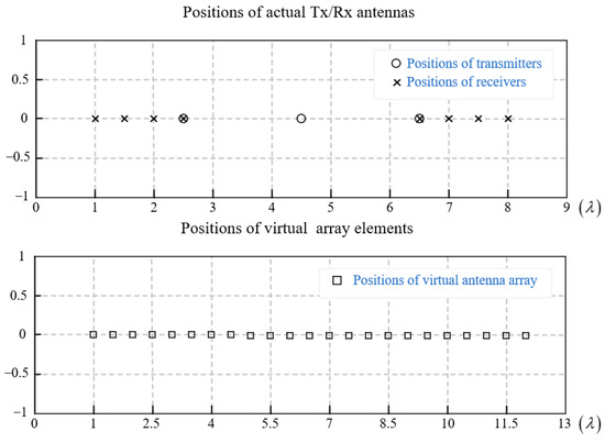
Figure 1.
The relationship between the real Tx/Rx antenna positions and the virtual array positions.
In Figure 1, the distances between the receivers and the transmitters are and , respectively. Using this special physical antenna configuration, we can generate a virtual linear array consisting of 23 elements with the interelement space . When the signal from the Tx antenna is reflected by an object at the angle with regard to the radar, the phase difference between elements is . Assuming that the aperture size of a single radar is w, then the signal of the ith element is
where
Taking the 2D-FFT along the t and i dimensions from Equation (4), we obtain
where u is the imaging result of . It is clear that Equation (7) includes both the distance and the angle information in a single radar, so we can image according to the formula. Furthermore, we expected that the angular resolution would be improved by using multiple radars. To build a distributed radar system, we put three radars in a line. The virtual array elements of the distributed radar system are shown in Figure 2, where is the virtual array length of a single radar and is the gap length between the radars. In particular, we set as equal to here. The virtual array is discontinuous because . Therefore, the traditional range-Doppler imaging method would result in problems, such as ghosting, grating lobes and side lobes, thereby reducing the image resolution.
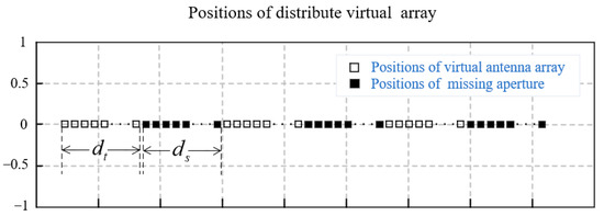
Figure 2.
The virtual array of the distributed FMCW MIMO radar system, with 86 virtual elements in and 86 missing virtual elements in .
The signal in Equation (4) is still continuous in the t dimension, which can be represented as below after range compression
For a distributed radar system, in Equation (8) can only complete the range compression if the FFT is used because y is discontinuous in the i dimension. Next, we tried to complete the azimuth compression. In matrix form, the relationship between the imaging result u and range compression result r can be rewritten as
where is the vector of the range compression and is the imaging result. denotes Gaussian noise with variance and is the discontinuous Fourier dictionary matrix related to i, which has the form below
where , and n is the number of radars.
In this context, the imaging problem can be converted into the problem of estimating u given r and H. For radar applications, the scene of interest is usually predominantly sparse. Due to the sparsity of u, the crux of the problem is to find a value for that satisfies Equation (9) and has as few non-zero elements as possible. By introducing the norm, can be estimated via the following optimization problem
where is the parameter to control the sparsity, and defines the number of non-zero elements in u.
2.2. Sparse Bayesian Learning Algorithm
Equation (9) is known as compressed sensing (CS) [27]. The problem to be solved with CS is that there exists a vector x and observation matrix H in advance, and we need to obtain u as accurately as possible. In this study, we needed to obtain the imaging vector u from the range compression vector r. Let M and N equal the number of rows and columns of H. Given the fact that M < N, Equation (9) is an ill-posed problem that has infinite solutions.
Sparse Bayesian learning has been widely used to solve CS reconstruction problems [38,39,40]. It assumes that r obeys a Gaussian likelihood , and is the variance in , so the problem is estimating the maximum likelihood of u and β. To avoid overfitting, a hierarchical Gaussian prior is applied to u, where is a vector of N hyperparameters corresponding to u. Next, let and have Gamma densities and . Through a series of transformations based on Bayesian theory, the solution can be obtained. The steps of the SBL algorithm are shown in Algorithm 1.
| Algorithm 1 Sparse Bayesian Learning (SBL algorithm) |
| 1: Input r, H, a, b, c and d. We set a = b =c = d = . Let M (N) equal the number of rows (columns) of H. 2: Initialize parameter . We set (), and Q and are determined according to Equations (12) and (13). 3: Set a threshold to determine if satisfies Equation (9). 4: while do 5: for i = 1: N do 6: 7: 8: end 9: 10: 11: (12) 12: (13) 13: (14) 14: end 15: Return |
From Algorithm 1, it is obvious that SBL needs a significant amount of computation owing to the iterative process. In particular, steps 12–14 account for almost all the computation and involve the inverse of the matrix Q.
3. LC-SBL Fast SBL Algorithm
Thanks to the Fourier matrix H, many of the multiplications of the matrices can be quickly figured out using the FFT process. Focusing on steps 12–14, we established a new decomposition of and developed LC-SBL algorithm.
In this section, we first give the equation for fast calculation of Q using the FFT. Next, we introduce the 2D Levinson–Durbin (L-D) algorithm to solve the linear system , where is a block vector for which the (i + 1)th element is the identity matrix I, while the rest of the elements are 0. Then, we reconstruct the inverse of Q by using x and s, where . Finally, the Vara algorithm and Wxper algorithm are employed to solve Equations (13) and (14) quickly.
3.1. Calculation Method for Matrix Q and 2D L-D Algorithm
Let , where . F is a Hermitian TBT matrix owing to the Fourier dictionary H, which has the following form:
Each submatrix is a w × w Toeplitz matrix
in can be computed as
where is the diagonal element of , . From Equation (20), we can see that can be quickly computed by using the N-points FFT with respect to the vector , so the matrix Q can be obtained directly through the FFT process. In addition, the main diagonal elements of Q are real numbers.
Let
satisfy these equations
Then, x, , y and have the following relationships
It is easy to conform Equations (25)–(27) by using the equation . We can obtain s and x efficiently using the 2D L-D algorithm. , y and can easily be obtained from x, and we can use them to decompose . The 2D L-D algorithm is summarized in Algorithm 2.
| Algorithm 2 Two-dimensional (2D) L-D algorithm |
| 1: Input and (similar to in F). 2: Initialize parameters W and Y as follows 3: for i = 2: w−1 do 4: 5: O is a zero matrix. 6: 7: end 8: 9: Return s, x |
3.2. Decomposition of Matrix
The 2D L-D algorithm can be used to efficiently calculate x and s, which means that , y and can also be obtained from x through Equations (25)–(27) without extra computation. Next, we use these block vectors to reconstruct the inverse of Q.
Let Z be the block cyclic lower shift matrix defined by
The cyclic displacement of [41] is given as
Since Q is a TBT matrix with a special structure, we can easily determine that
could be an arbitrary w × w matrix. It is easy to observe that if Q is a block circulant matrix. There exists a common relationship between the displacement of Q and the displacement of , and the connection is as follows
Moreover, Equation (31) and the cyclic displacement allow us to calculate the inverse of Q. We obtain the following theorem [42].
THEOREM: If the cyclic displacement of Q can be rewritten as the sum
where , are given block vectors, the following formula exists
Let . The matrix L(z) is a block lower triangular matrix, the form of which is defined by
C(z) is a circulant matrix with the form
is a circulant matrix that has the same last row as Q.
Let
satisfy the following equations
With the help of Equation (31), can be rewritten as
According to the previous theorem, the matrix can be represented as
where
Given the fact that
Equation (44) can be simplified as
Solving Equations (41) and (42) directly requires significant amounts of computation. A fast method to obtain and exists.
We obtain
Reference [42] provides the following property for any invertible TB matrix
As a consequence, and are the solutions for Equations (41) and (42). Furthermore, we obtain
and
Therefore, we can reconstruct the inverse of Q by using x, , y and . Due to the relationships between them, Equation (47) can be written as
3.3. Wxpet Algorithm
From the previous section, we know that the inverse of Q can be decomposed into the sum of products of block lower triangular Toeplitz matrices and block circulant matrices. With this method, we can calculate Equations (13) and (14) by using linear convolution and circulant convolution. Q is a n × n block matrix, the elements of which are a w × w square matrix. As , directly bringing Q into Equations (13) and (14) will lead to numerous FFT steps, and every vector operated with the FFT will be short. To reduce FFT operations and accelerate the algorithm, we can define the permutation matrix S by
where is the (i +1)th column of I. Let
Here, R is a w × w Hermitian TBT matrix, the elements of which are n × n square matrices. We can use the previous method to decompose it. According to Equation (53), R can be rewritten briefly as
Then, can be expressed as
We use to denote the ith column of and to denote the ith row of
The matrix can be rewritten as
where T represents the w × w lower triangular Toeplitz matrix
and M represents the w × w circulant matrix
T and M can be obtained from x and s using Equations (57)–(60). Consequently, the multiplication of the inverse of Q by r in Equation (14) can be computed as several T matrices multiplied by r and several M matrices multiplied by r
Linear convolution and circular convolution can be used to calculate v, which only requires the first rows of T and M. Additionally, due to the Fourier dictionary H, we can divide v into n equal segments and fill each segment with m zeros to perform the IFFT and obtain
The sizes of the zero vector and depend on and . The fast algorithm for the calculation of is summarized below (Algorithm 3).
| Algorithm 3 Compute (Wxpet algorithm) |
| 1: Input x, s and r. 2: for t = 1:2; (the first block column of ), (the first block column of ) 3: for i = 1:n 4: for j = 1:n 5: end 6: for j = 1:n discard redundant convolution results 7: end 8: 9: end 10: end 11: 12: 13: Return |
3.4. Vara Algorithm
For a block matrix, we define the sum of matrices on the diagonal of as , and the index c is 0 when the diagonal is the main diagonal and it is plus 1 when the diagonal moves up one step. The rule also applies to simple matrices. In this way, the number denotes the sum of the dth diagonal of the matrix .
As is a Hermitian matrix, we have
The sum of all diagonals in the upper half of matrix can be computed by
For matrix , the sums of all diagonals can be computed as
where has the form shown in Equation (61), the first column of which is , and q is a coefficient vector determined by k
Let
We need to pad zero in K, and then we can get
We just need to add one zero number in terms of = , and then h can be quickly computed using the FFT and IFFT
The Vara algorithm is shown below (Algorithm 4). Diag(b, a) means the diagonal elements of the multiplication of circulant matrix T and Toeplitz matrix M should be calculated according to Equations (67)–(71), in which the first row of T is b and the first row of M is a.
| Algorithm 4 Compute h (Vara Algorithm) |
| 1: Input x and s 2: for t = 1:2 the first block column of , the first block column of 3: for i = 1:n 4: for j = 1:n 5: end 6: for s = 1:n 7: += [zeros(2m−1, t−1) Diag ] 8: end 9: 10: end 11: 12: We obtain and by adding zeros in vector K 13: 14: Return h |
We focus on multiplication only because addition and subtraction operations are much faster than multiplication operations. We can calculate h and v directly by multiplying the matrices, requiring computations. In comparison, the 2D L-D algorithm, Wxpet algorithm and Vara algorithm need about computations in total. In the next section, we describe the simulation run with these methods, and we compare the number of calculations required and the computational time.
4. Simulation and Measured-Data Processing Results
We used simulation and measured data to demonstrate the advantages of LC-SBL in improving imaging resolution and saving computation time. In addition, the orthogonal matching pursuit (OMP) [26] algorithm, the fast IAA (FIAA) [24] algorithm and Student’s T prior-based efficient SBL (S-ESBL) [34] algorithm were emulated for comparison.
We defined normalized root mean square errors (nRMSE) to evaluate the reconstruction performance of the algorithms in simulation. The nRMSE is computed as
We simulated a radar system with 516 elements composed of six radars; each radar had 86 array elements and the spacing between adjacent elements was half the wavelength. We made the center of the 516 elements the origin. To obtain the gapped data, we manually abandoned the second, fourth and sixth radars’ data after collecting it. The radar parameters were as follows: the central frequency was 77 GHz, the bandwidth was 3 GHz, the sampling rate was 16,000 kHz, the number of ADC samples was 800 and the signal-to-noise ratio (SNR) was set to 15 dB.
4.1. Simulation of Angular Resolution of Several Algorithms
In the first simulation, all observed data were obtained from 4 sets of points 30 m away. The intervals between groups were 0.5 m, and the gapped distances between points in each group were 0.05 m, 0.1 m, 0.15 m and 0.2 m, respectively. For the SBL, S-ESBL and LCSBL algorithms, the hyperparameters were set as a = b = c = d = , and γ and β were initialized as and . The maximum number of iterations was set to 1000. For the SBL and LC-SBL algorithms, the convergence δ was set to 10−3. In particular, δ was set to 10−4 in the S-ESBL algorithms due to the slow convergence speed. Generally speaking, the FIAA algorithm converges to the best case when the number of iterations reaches 15 [24], so we set 15 iterations here.
Figure 3 shows three sets of simulation results obtained with conventional SBL to assess angular resolution. Figure 3b–g shows the images of the 86 elements, 516 elements and distributed radar system. In addition, the one-dimensional azimuth profiles of the 16 targets are displayed. Due to the small amount data for single radars, the resolution of Figure 3b is very poor, and the points of the fourth group cannot even be perfectly distinguished. In contrast, the data imaging effect of the 516 elements was excellent. It can also be seen that the points of each group were successfully identified, and even the points with a distance of 0.05 m can be distinguished accurately. In addition, the distributed radar system also identified every point successfully. With the conventional SBL algorithm, the angular resolution of the distributed radar system was comparable to that of a radar with 516 array elements.

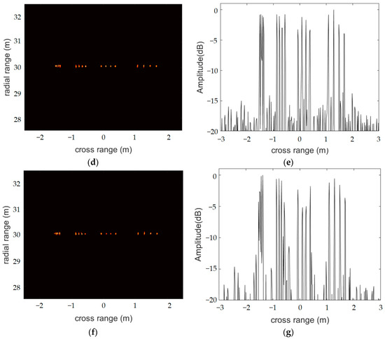
Figure 3.
(a) Image model. Imaging results and azimuth profiles of 86 element radar (b,c), 516 element radar (d,e) and distributed radar system (f,g) obtained by using conventional SBL algorithm.
In this experiment, we wanted to evaluate the imaging performance of the distributed radar system with the FIAA, OMP and S-ESBL algorithms. Figure 4 demonstrates the imaging results and the azimuth profiles. From Figure 4, we can see that the FIAA and S-ESBL algorithms achieved high accuracy. They clearly identified targets in both the second and third groups, but only three targets were displayed in the first group. This shows that their resolutions at 30 m were not as good as that of a 516 array element radar. Moreover, although the imaging result for the OMP algorithm had no side lobes, it was very unstable, and the target image with low sparsity was blurred. The LC-SBL algorithm is a fast version of the SBL algorithm, and the result shown in Figure 4g is as clear as that in Figure 3f.
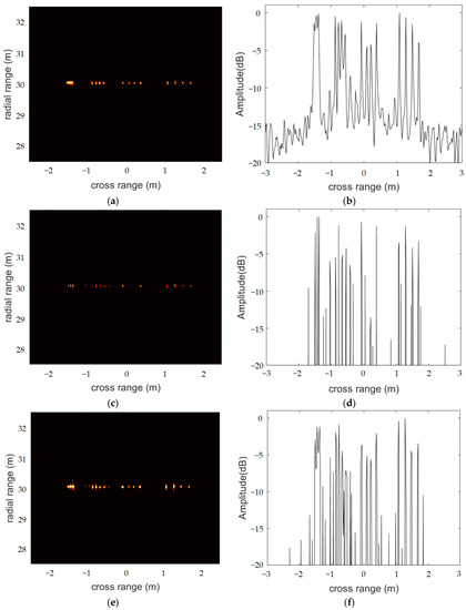
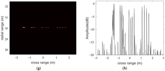
Figure 4.
Imaging results and azimuth profiles using the FIAA (a,b), OMP (c,d), S-ESBL (e,f) and LC-SBL (g,h) algorithms for a distributed radar system.
4.2. nRMSE Values and Running Times of the Algorithms
To determine the nRMSE and running time of each algorithm, we performed 1000 Monte Carlo experiments with different signal-to-noise ratios. Table 1 and Figure 5 illustrate the results. In this experiment, we randomly selected 30 random frequencies from 516 azimuth profiles in the same range profile and transformed the frequency domain data to the time domain to obtain the data collected by the distributed radar system.

Table 1.
The average computational times of the OMP, FIAA, SBL, S-ESBL and LC-SBL algorithms with a 10 dB SNR.
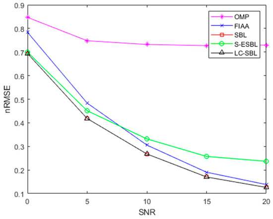
Figure 5.
The average nRMSE of the images obtained using the OMP, FIAA, SBL, S-ESBL and LC-SBL algorithms.
From Table 1 and Figure 5, we can see that the OMP algorithm was extremely fast, but its nRMSE value remained around 0.8 and hardly changed with different signal-to-noise ratios. Among the other algorithms, the LC-SBL algorithm not only had the lowest nRMSE but also required the shortest time. The FFD-SBL algorithm [43] is also a kind of fast SBL algorithm based on G-S decomposition of a TBT matrix without any approximations. It had the same nRMSE as the LC-SBL algorithm but took a little longer.
4.3. Measured Data Imaging
Finally, we used measured data from two scenes to demonstrate the performance of the LC-SBL algorithm in improving the angular resolution, with scene one being composed of five corner reflectors and scene two of town normal bikes. An inevitable millimeter-level error was expected in the placement of the radar, which would have caused a certain phase error for millimeter waves. Therefore, we applied the self-focus algorithm [44,45,46] after imaging. The distributed radar system consisted of three MMWAVCAS-RF-EVM development kits produced by Texas Instruments. The width of each radar was and the distance between radars was ; thus, we had = 17.2 cm. Each radar board had 9 transmitting antennas and 12 receiving antennas, forming 86 apertures in the azimuth direction. The size of each aperture equaled 0.5. We calculated the angular resolution as 1.35° using the formula
where is the wavelength and D is the length of the whole aperture array.
In the experiment, we set the start frequency as 77 GHz, the bandwidth as 1.5 GHz, the sampling frequency as 16,000 KHz and the number of sampling points for one chirp as 512. Figure 6a shows the distributed radar system, and Figure 6b shows the measurement targets for scene one. We measured five corner reflections, imaging at a distance of 35.5 m from the radar system, with an interval between pairs of corner reflectors of 14 cm. The resolution of the single radars at 35.5 m was about 80 cm. The virtual aperture array length of the distributed radar system was six times that of a single radar, so it could theoretically achieve a resolution of 13.4 cm. Figure 6c,e show the images of the whole scene and the targets imaged by the single-radar system. Figure 6e,f show the distributed radar system imaging results for the five corner reflections obtained with the FIAA, OMP, S-ESBL and LC-SBL algorithms. From Figure 6, we can see that the single-radar SBL could not distinguish corner reflectors at all. In the distributed radar system, the OMP algorithms could only image four targets, and the imaging results for the FIAA and S-ESBL algorithms were somewhat blurred; they could not clearly show the five targets. In contrast, the LC-SBL algorithm successfully identified every corner reflector in the same scene.
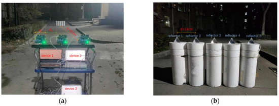
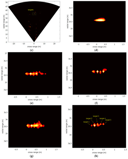
Figure 6.
Scene one: (a) photograph of distributed radar system, (b) photograph of five corner reflectors, (c) single-radar SBL imaging result. Zoomed-in imaging of targets with the single-radar system and SBL algorithm (d), the distributed radar system and FIAA algorithm (e), the distributed radar system and OMP algorithm (f), the distributed radar system and S-ESBL algorithm (g) and the distributed radar system and LC-SBL algorithm (h).
The next scene depicted two bikes next to each other, as shown in Figure 7b. The parameters of the radar were set the same as scene 1. From Figure 7, we can see that the imaging result of the single-radar SBL was very poor, and the number and shapes of the bicycles cannot be distinguished because of the low resolution. For the distributed radar system, the results displayed by the OMP algorithm were obviously not as good as the other algorithms. The FIAA algorithm displayed the image as clearly as the S-ESBL algorithm, and the performance of the LC-SBL algorithm was the best, the silhouettes of the two bikes being perfectly distinguished.
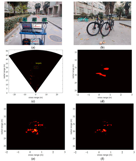
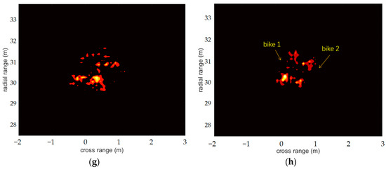
Figure 7.
Scene two: (a) photograph of distributed radar system, (b) photograph of two bikes, (c) single-radar SBL imaging result. Zoomed-in imaging of targets with the single-radar system and SBL algorithm (d), distributed radar system and FIAA algorithm (e), distributed radar system and OMP algorithm (f), distributed radar system and S-ESBL algorithm (g) and distributed radar system and LC-SBL algorithm (h).
5. Conclusions
In this study, a novel fast SBL algorithm, referred to as the LC-SBL algorithm, was developed for distributed FMCW MIMO radar system imaging to obtain high angular resolution. To address the problem of high computational complexity in SBL, we proposed a new decomposition method for the inverse of a TBT matrix. With this method, several important parameters can be quickly calculated using the FFT. The performance of the LC-SBL algorithm was much better than that of the OMP algorithm. Compared to the FIAA and S-ESBL algorithms, LC-SBL not only performed better but also required less time. Moreover, the LC-SBL algorithm was more efficient than the FFD-SBL algorithm.
Author Contributions
Conceptualization, F.D.; Data curation, Y.L.; Investigation, Y.L. and Y.W.; Methodology, F.D. and Y.L.; Project administration, F.D.; Software, Y.L.; Visualization, Y.L.; Supervision, H.C.; Resources, H.C.; Writing—original draft, Y.L.; Writing—review and editing, F.D. and Y.W. All authors have read and agreed to the published version of the manuscript.
Funding
This work was supported by the National Natural Science Foundation of China under grant no. 62271363.
Data Availability Statement
Not applicable.
Conflicts of Interest
The authors declare no conflict of interest.
References
- Wei, S.; Zhou, Z.; Wang, M.; Wei, J.; Liu, S.; Shi, J.; Zhang, X.; Fan, F. 3DRIED: A High-Resolution 3-D Millimeter-Wave Radar Dataset Dedicated to Imaging and Evaluation. Remote Sens. 2021, 13, 3366. [Google Scholar] [CrossRef]
- Gottinger, M.; Hoffmann, M.; Christmann, M. Coherent automotive radar networks: The next generation of radar-based im-aging and mapping. IEEE J. Microw. 2021, 1, 149–163. [Google Scholar] [CrossRef]
- Wang, Z.; Miao, X.; Huang, Z.; Luo, H. Research of Target Detection and Classification Techniques Using Millimeter-Wave Radar and Vision Sensors. Remote Sens. 2021, 13, 1064. [Google Scholar] [CrossRef]
- Munte, N.; Lazaro, A.; Villarino, R.; Girbau, D. Vehicle Occupancy Detector Based on FMCW mm-Wave Radar at 77 GHz. IEEE Sensors J. 2022, 22, 24504–24515. [Google Scholar] [CrossRef]
- Zhang, B.; Xu, G.; Zhou, R.; Zhang, H.; Hong, W. Multi-Channel Back-Projection Algorithm for Mmwave Automotive MIMO SAR Imaging with Doppler-Division Multiplexing. IEEE J. Sel. Top. Signal Process. 2022, PP, 1–13. [Google Scholar] [CrossRef]
- Schwarz, D.; Riese, N.; Dorsch, I.; Waldschmidt, C. System Performance of a 79 GHz High-Resolution 4D Imaging MIMO Radar with 1728 Virtual Channels. IEEE J. Microw. 2022, 2, 637–647. [Google Scholar] [CrossRef]
- Yang, B.; Zhang, H.; Chen, Y.; Zhou, Y.; Peng, Y. Urban Traffic Imaging Using Millimeter-Wave Radar. Remote Sens. 2022, 14, 5416. [Google Scholar] [CrossRef]
- Liu, P.; Yu, G.; Wang, Z.; Zhou, B.; Chen, P. Object Classification Based on Enhanced Evidence Theory: Radar–Vision Fusion Approach for Roadside Application. IEEE Trans. Instrum. Meas. 2022, 71, 5006412. [Google Scholar] [CrossRef]
- Huang, X.; Dong, X.; Ma, J.; Liu, K.; Ahmed, S.; Lin, J.; Qiu, B. The Improved A* Obstacle Avoidance Algorithm for the Plant Protection UAV with Millimeter Wave Radar and Monocular Camera Data Fusion. Remote Sens. 2021, 13, 3364. [Google Scholar] [CrossRef]
- Wilson, A.N.; Kumar, A.; Jha, A.; Cenkeramaddi, L.R. Embedded Sensors, Communication Technologies, Computing Platforms and Machine Learning for UAVs: A Review. IEEE Sensors J. 2021, 22, 1807–1826. [Google Scholar] [CrossRef]
- Zhao, Y.; Yarovoy, A.; Fioranelli, F. Angle-Insensitive Human Motion and Posture Recognition Based on 4D Imaging Radar and Deep Learning Classifiers. IEEE Sensors J. 2022, 22, 12173–12182. [Google Scholar] [CrossRef]
- Ando, T.; Kidera, S. Accurate Micro-Doppler Analysis by Doppler and $k$-Space Decomposition for Millimeter Wave Short-Range Radar. IEEE J. Sel. Top. Appl. Earth Obs. Remote. Sens. 2022, 15, 2503–2518. [Google Scholar] [CrossRef]
- Antolinos, E.; García-Rial, F.; Hernández, C.; Montesano, D.; Godino-Llorente, J.I.; Grajal, J. Cardiopulmonary Activity Mon-itoring Using Millimeter Wave Radars. Remote Sens. 2020, 12, 2265. [Google Scholar] [CrossRef]
- Li, G.; Ge, Y.; Wang, Y.; Chen, Q.; Wang, G. Detection of Human Breathing in Non-Line-of-Sight Region by Using mmWave FMCW Radar. IEEE Trans. Instrum. Meas. 2022, 71, 8006311. [Google Scholar] [CrossRef]
- Zhang, Q.; Zhang, Y.; Zhang, Y.; Huang, Y.; Yang, J. A Sparse Denoising-Based Super-Resolution Method for Scanning Radar Imaging. Remote Sens. 2021, 13, 2768. [Google Scholar] [CrossRef]
- Zhang, Q.; Zhang, Y.; Huang, Y.; Zhang, Y.; Pei, J.; Yi, Q.; Li, W.; Yang, J. TV-Sparse Super-Resolution Method for Radar Forward-Looking Imaging. IEEE Trans. Geosci. Remote. Sens. 2020, 58, 6534–6549. [Google Scholar] [CrossRef]
- Cong, J.; Wang, X.; Lan, X.; Huang, M.; Wan, L. Fast Target Localization Method for FMCW MIMO Radar via VDSR Neural Network. Remote Sens. 2021, 13, 1956. [Google Scholar] [CrossRef]
- Nanzer, J.A.; Mghabghab, S.R.; Ellison, S.M.; Schlegel, A. Distributed Phased Arrays: Challenges and Recent Advances. IEEE Trans. Microw. Theory Tech. 2021, 69, 4893–4907. [Google Scholar] [CrossRef]
- Coutts, S.; Cuomo, K.; McHarg, J. Distributed coherent aperture measurements for next generation BMD radar. In Proceedings of the Fourth IEEE Workshop on Sensor Array and Multichannel Processing, Waltham, MA, USA, 12–14 July 2006; pp. 390–393. [Google Scholar]
- Seo, J.; Hwang, S.; Hong, Y.-G.; Park, J.; Hwang, S.; Byun, W.-J. Bayesian Matching Pursuit-Based Distributed FMCW MIMO Radar Imaging. IEEE Syst. J. 2020, 15, 4623–4634. [Google Scholar] [CrossRef]
- Mansour, H.; Liu, D.; Kamilov, U.S.; Boufounos, P.T. Sparse Blind Deconvolution for Distributed Radar Autofocus Imaging. IEEE Trans. Comput. Imaging 2018, 4, 537–551. [Google Scholar] [CrossRef]
- Cuomo, K.M.; Piou, J.E.; Mayhan, J.T. Ultra-wideband coherent processing. Linc. Lab. J. 1997, 10, 203–222. [Google Scholar]
- Larsson, E.G.; Li, J. Spectral analysis of periodically gapped data. IEEE Trans. Aerosp. Electron. Syst. 2003, 39, 1089–1097. [Google Scholar] [CrossRef]
- Glentis, G.-O.; Jakobsson, A. Efficient Implementation of Iterative Adaptive Approach Spectral Estimation Techniques. IEEE Trans. Signal Process. 2011, 59, 4154–4167. [Google Scholar] [CrossRef]
- Kang, M.S.; Lee, S.J.; Lee, S.H. ISAR imaging of high-speed maneuvering target using gapped stepped-frequency waveform and compressive sensing. IEEE Trans. Image Process. 2017, 26, 5043–5056. [Google Scholar] [CrossRef] [PubMed]
- Tropp, J.A.; Gilbert, A.C. Signal Recovery from Random Measurements via Orthogonal Matching Pursuit. IEEE Trans. Inf. Theory 2007, 53, 4655–4666. [Google Scholar] [CrossRef]
- Donoho, D.L. Compressed sensing. IEEE Trans. Inf. Theory 2006, 52, 1289–1306. [Google Scholar] [CrossRef]
- Ji, S.; Xue, Y.; Carin, L. Bayesian compressive sensing. IEEE Trans. Signal Process. 2008, 56, 2346–2356. [Google Scholar] [CrossRef]
- Shutin, D.; Buchgraber, T.; Kulkarni, S.R.; Poor, H.V. Fast Variational Sparse Bayesian Learning with Automatic Relevance Determination for Superimposed Signals. IEEE Trans. Signal Process. 2011, 59, 6257–6261. [Google Scholar] [CrossRef]
- Tipping, M.E.; Faul, A.C. Fast marginal likelihood maximisation for sparse Bayesian models. In Proceedings of the International Workshop on Artificial Intelligence and Statistics, Key West, FL, USA, 3–6 January 2003; Volume 1, pp. 276–283. [Google Scholar]
- Al-Shoukairi, M.; Schniter, P.; Rao, B.D. A GAMP-Based Low Complexity Sparse Bayesian Learning Algorithm. IEEE Trans. Signal Process. 2017, 66, 294–308. [Google Scholar] [CrossRef]
- Tan, X.; Li, J. Computationally Efficient Sparse Bayesian Learning via Belief Propagation. IEEE Trans. Signal Process. 2010, 58, 2010–2021. [Google Scholar] [CrossRef]
- Duan, H.; Yang, L.; Fang, J.; Li, H. Fast Inverse-Free Sparse Bayesian Learning via Relaxed Evidence Lower Bound Maximization. IEEE Signal Process. Lett. 2017, 24, 774–778. [Google Scholar] [CrossRef]
- Zhou, W.; Zhang, H.-T.; Wang, J. An Efficient Sparse Bayesian Learning Algorithm Based on Gaussian-Scale Mixtures. IEEE Trans. Neural Netw. Learn. Syst. 2021, 33, 3065–3078. [Google Scholar] [CrossRef] [PubMed]
- Tang, Y.; Lu, Y. Single transceiver-based time division multiplexing multiple-input–multiple-output digital beamforming radar system: Concepts and experiments. IET Radar Sonar Navig. 2014, 8, 368–375. [Google Scholar] [CrossRef]
- Robey, F.C.; Coutts, S.; Weikle, D. MIMO radar theory and experimental results. Conf. Rec. Thirty-Eighth Asilomar Conf. Signals Syst. Comput. 2004, 1, 300–304. [Google Scholar]
- Sun, H.; Brigui, F.; Lesturgie, M. Analysis and comparison of MIMO radar waveforms. In Proceedings of the 2014 International Radar Conference, Lille, France, 13–17 October 2014; pp. 1–6. [Google Scholar] [CrossRef]
- Tipping, M.E. Sparse Bayesian learning and the relevance vector machine. J. Mach. Learn. Res. 2001, 1, 211–244. [Google Scholar]
- Zhang, Z.; Rao, B.D. Sparse Signal Recovery with Temporally Correlated Source Vectors Using Sparse Bayesian Learning. IEEE J. Sel. Top. Signal Process. 2011, 5, 912–926. [Google Scholar] [CrossRef]
- Wipf, D.; Rao, B. Sparse Bayesian Learning for Basis Selection. IEEE Trans. Signal Process. 2004, 52, 2153–2164. [Google Scholar] [CrossRef]
- Gohberg, I.; Olshevsky, V. Circulants, displacements and decompositions of matrices. Integral Equ. Oper. Theory 1992, 15, 730–743. [Google Scholar] [CrossRef]
- Lv, X.-G.; Huang, T.-Z. The Inverses of Block Toeplitz Matrices. J. Math. 2013, 2013, 207176. [Google Scholar] [CrossRef]
- Dai, F.; Wang, Y.; Hong, L. Gohberg-Semencul Factorization-Based Fast Implementation of Sparse Bayesian Learning with a Fourier Dictionary. IEEE Trans. Geosci. Remote. Sens. 2022, 60, 1–15. [Google Scholar] [CrossRef]
- Zhang, S.; Liu, Y.; Li, X. Autofocusing for Sparse Aperture ISAR Imaging Based on Joint Constraint of Sparsity and Minimum Entropy. IEEE J. Sel. Top. Appl. Earth Obs. Remote. Sens. 2016, 10, 998–1011. [Google Scholar] [CrossRef]
- Xi, L.; Guosui, L.; Ni, J. Autofocusing of ISAR images based on entropy minimization. IEEE Trans. Aerosp. Electron. Syst. 1999, 35, 1240–1252. [Google Scholar] [CrossRef]
- Kang, M.-S.; Bae, J.-H.; Lee, S.-H.; Kim, K.-T. Efficient ISAR autofocus via minimization of Tsallis Entropy. IEEE Trans. Aerosp. Electron. Syst. 2017, 52, 2950–2960. [Google Scholar] [CrossRef]


Disclaimer/Publisher’s Note: The statements, opinions and data contained in all publications are solely those of the individual author(s) and contributor(s) and not of MDPI and/or the editor(s). MDPI and/or the editor(s) disclaim responsibility for any injury to people or property resulting from any ideas, methods, instructions or products referred to in the content. |
© 2023 by the authors. Licensee MDPI, Basel, Switzerland. This article is an open access article distributed under the terms and conditions of the Creative Commons Attribution (CC BY) license (https://creativecommons.org/licenses/by/4.0/).