Article

Integrating UAV-Derived Information and WorldView-3 Imagery for Mapping Wetland Plants in the Old Woman Creek Estuary, USA

1
School of Earth, Environment and Society, Bowling Green State University, Bowling Green, OH 43403, USA
2
Department of Environmental Health Science, University of Michigan, Ann Arbor, MI 48109, USA
3
Equifax, 11432 Lackland Rd., St. Louis, MO 63146, USA
4
Department of Computer Science, Bowling Green State University, Bowling Green, OH 43403, USA
*
Author to whom correspondence should be addressed.
Remote Sens. 2023, 15(4), 1090; https://doi.org/10.3390/rs15041090
Submission received: 3 December 2022 / Revised: 11 February 2023 / Accepted: 14 February 2023 / Published: 16 February 2023

Abstract

:
The classification of wetland plants using unmanned aerial vehicle (UAV) and satellite synergies has received increasing attention in recent years. In this study, UAV-derived training and validation data and WorldView-3 satellite imagery are integrated in the classification of five dominant wetland plants in the Old Woman Creek (OWC) estuary, USA. Several classifiers are explored: (1) pixel-based methods: maximum likelihood (ML), support vector machine (SVM), and neural network (NN), and (2) object-based methods: Naïve Bayes (NB), support vector machine (SVM), and k-nearest neighbors (k-NN). The study evaluates the performance of the classifiers for different image feature combinations such as single bands, vegetation indices, principal components (PCs), and texture information. The results showed that all classifiers reached high overall accuracy (>85%). Pixel-based SVM and object-based NB exhibited the best performance with overall accuracies of 93.76% and 93.30%, respectively. Insignificantly lower overall accuracy was achieved with ML (92.29), followed by NN (90.95) and object-oriented SVM (90.61). The k-NN method showed the lowest (but still high) accuracy of 86.74%. All classifiers except for the pixel-based SVM required additional input features. The pixel-based SVM achieved low errors of commission and omission, and unlike the other classifiers, exhibited low variability and low sensitivity to additional image features. Our study shows the efficacy of combining very high spatial resolution UAV-derived information and the super spectral observation capabilities of WorldView-3 in machine learning for mapping wetland vegetation.

1. Introduction

Freshwater estuaries and wetlands are among the most productive and biodiverse ecosystems that provide beneficial services for people and wildlife. Along with socio-economic contributions to society such as fishing and recreation, wetlands improve the water quality of nearby water bodies, mitigate floods in coastal areas, sequestrate carbon, and maintain nutrient cycling from nearby agriculture areas [1]. In recent decades, a dramatic decline in wetlands has been observed due to the combined effects of climate change and human influence [2,3]. Wetland plants play one of the most important roles in the food chain and energy flow of wetlands. They provide critical habitat to diverse communities from bacteria to fish and birds, and they are seen as a biological indicator of wetlands’ health [4]. As a result of major hydrological changes, human interaction, urbanization, and the increase in agricultural areas, urban wetlands’ native species are often replaced with invasive plants, which have negative implications on the ecosystem conditions [5]. Therefore, a better understanding of the spatial distribution of wetland plants and their classification is critical for wetland monitoring and their sustainable development.
Satellite and airborne multispectral imagery have been widely used to collect spatial and temporal information about wetland ecosystems at different scales. While the use of Landsat [6,7,8] and Sentinel-2 imagery [9,10] is common and considered a standard approach in mapping wetland vegetation [11], their relatively coarse spatial resolution remains a challenge. Thus, high-resolution images (≤5 m spatial resolution) are attracting interest from geospatial scientists who have recognized the advantages of their spectral information for detecting small features [12]. To use the advantage of high-resolution satellite sensors, the Commercial Small-satellite (Smallsat) Data Acquisition (CSDA) program ensures a cost-effective means of monitoring wetlands [13]. Ref. [14] used RapidEye images to classify wetland vegetation communities in iSimangaliso Wetland Park with a high overall accuracy of 86%. Refs. [15,16] showed the great potential of high-resolution QuickBird and IKONOS imagery in mapping plant communities and monitoring invasive plants in the Hudson River estuary by achieving the overall accuracy ranges of 64.9–73.6% and 45–77%, respectively. High classification accuracies were reached in several studies where WorldView-2 was used [17,18]. Ref. [19] used WorldView-3 to classify wetland vegetation from the Millrace Flats Wildlife Management Area with a high overall accuracy of 93.33%. High accuracies were achieved with WorldView-3 in studies conducted by [20] over the Mai Po Nature Reserve of Hong Kong (up to 94.4%), and by [21] over the Akgol wetland area of Konya, Turkey (up to 96%).
In recent years, the use of an unmanned aerial vehicle (UAV) for mapping and monitoring wetland plants is seen as an economical way of obtaining remote sensing images at any desired time, and as a great addition to remote sensing research due to very high (sub-meter) spatial resolution [22,23,24]. UAVs are also seen as an alternative to the tedious fieldwork required to conduct and assess supervised classification. Due to on-demand remote sensing capabilities and very high spatial resolution, UAV images can be used to validate airborne and satellite data with a minimal disturbance to ecosystems [12,25]. With the development of UAV technology, a new idea of fusing and combining satellite imagery with UAV data or UAV-derived information using different strategies has been steadily emerging since 2008. In the scientific literature review, ref. [25] identified four main strategies of synergy between UAV and satellite imagery used in more than a hundred peer-reviewed articles across different fields: data comparison, multiscale explanation, data fusion, and model calibration. In the ‘data comparison’ strategy, the complementary natures of UAV and satellite data, such as a larger extent of satellite and very fine spatial resolution of UAV imagery, are exploited for the identification of features. The ‘multiscale explanation’ strategy combines information acquired at different scales to interpret data by capturing regional spatial and temporal trends with satellites and extracting fine features with UAVs. The strongest synergy between UAV and satellite data is obtained in ‘data fusion’, where different spatial, spectra, and temporal information of each data source are used to derive a new dataset. In the ‘model calibration’ strategy, UAV imagery is used to calibrate and validate satellite data, for instance, in the process of supervised classification. Furthermore, the study of [25] found that the synergy between UAV and satellite imagery was largely utilized in studies related to agriculture [26,27], forest [28], or land cover [29], and that the concept is under-exploited in wetland-related studies. Classification of wetland vegetation is mainly performed by combining WorldView-2 imagery and LiDAR data [30] or Landsat 8 OLI, ALOS-1 PALSAR, Sentinel-1, and LiDAR-derived topographic metrics [31,32], and only a handful of wetland-related studies have considered the UAV and satellite synergy. The approach was shown to be promising in the studies of [12,33], where UAV-derived information was combined with the WorldView-3 and RapidEye or fused with the sub-meter wideband multispectral satellite JL101K imagery, respectively. It is expected that UAV imagery will be progressively used in the process of data fusion with satellite data and/or for their calibration and validation.
The importance of machine learning techniques in the classification of wetland vegetation has been recognized for some time already. Machine learning techniques can handle non-linearity and complex training data that are typical for wetlands as well as complex relations between multi-source input data and estimation of parameters [25]. However, their performance cannot be easily generalized as the results depend on training data, input features, and number of classes. Methods such as random forest and decision trees [30,34], rule-based [21,35], support vector machine [12,18,20,21,36,37], k-Nearest Neighbor [17], and neural network [19,22] are now commonly used for different combinations of input features. For instance, ref. [12] considered texture, normalized difference vegetation index, LiDAR, and digital elevation model (DEM) to improve classification accuracy in the UAV-WorldView-3 integrated approach using the SVM while [19] reported that the principal component analysis (PC)-based feature selection technique and vegetation indices were effective in improving classification accuracy using the rule-based method and SVM classifiers to classify WorldView-3 imagery.
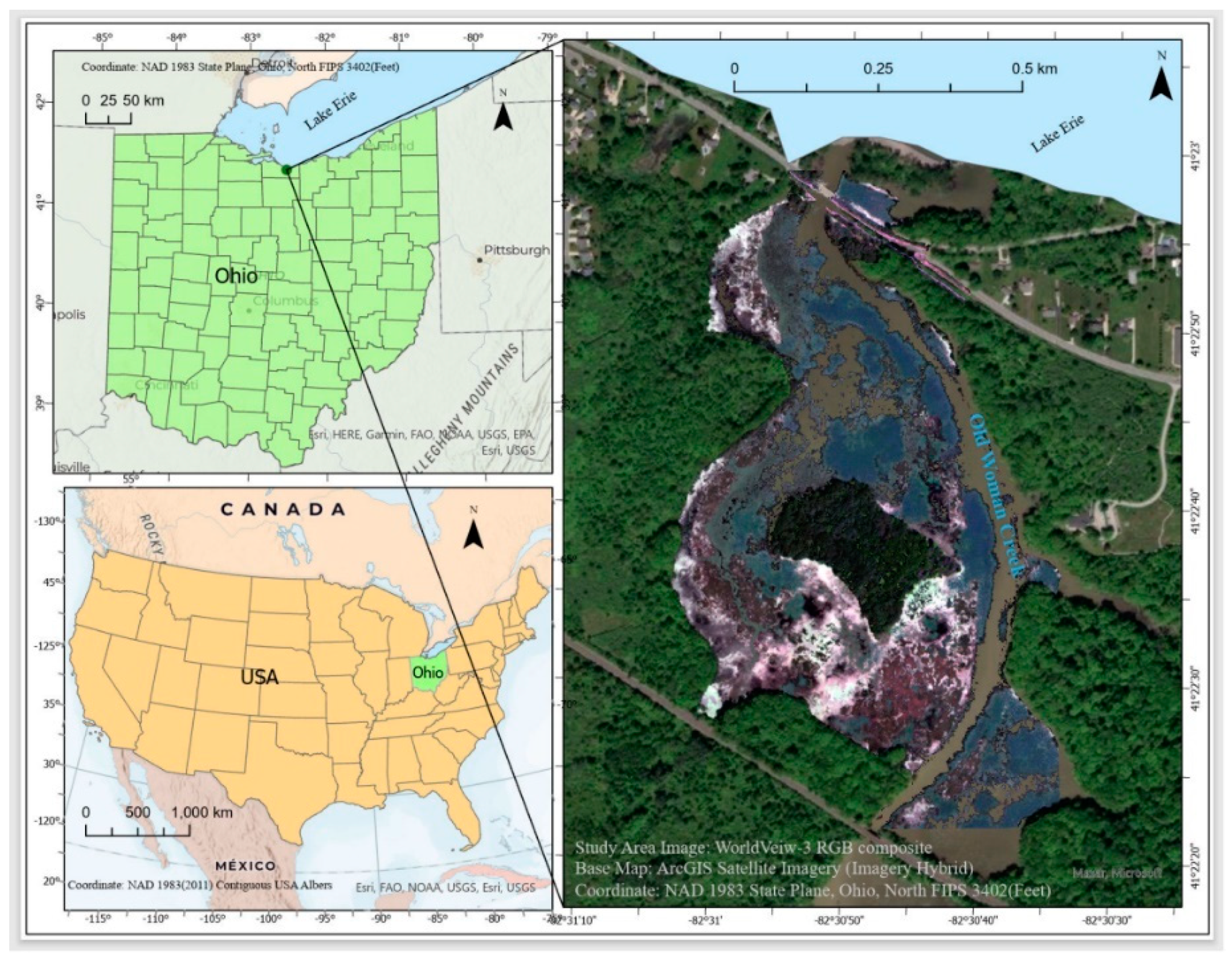
To demonstrate the ability of the very high spatial resolution of UAV-derived information in providing complementary information to the super spectral observation capabilities of WorldView-3, the current study underlines the importance of classifying wetland plants using machine learning techniques and the UAV-WorldView-3 integrated approach. The focus is on mapping five dominant wetland plants in the Old Woman Creek (OWC) estuary, USA, while using a UAV image to train and validate an array of input features and machine learning algorithms to classify WorldView-3 satellite imagery. The goal is to contribute toward filling research gaps in the classification of wetland plants based on the integration of UAV and high-resolution satellite imagery while selecting the best combinations of spectral information, including single bands, vegetation indices, and statistical features such as texture and principal components (PCs). Two classification approaches used in this study are: (1) pixel-based classification using maximum likelihood (ML), support vector machine (SVM), and neural network (NN) classifiers, and (2) object-based classification using naïve Bayes (NB), support vector machine (SVM), and k-nearest neighbors (k-NN) classifiers. The aim is to compare the performance of parametric (ML, NN, NB) and nonparametric classifiers (SVM, k-NN), and to compare the performance of the same classifier (SVM) for both the pixel- and object-based approaches.

2. Data and Methods

2.1. Study Area

The Old Woman Creek (OWC) estuary is located at the drowned mouth of a small tributary (41°22′34″N, 82°30′42″W) to Lake Erie (Figure 1) and was designated as the national estuarine research reserve in 1980. The estuary covers an area of approximately 42.81 km [38]. The water depth is less than 0.5 m in most of the estuary, although it can reach up to 3.6 m in the inlet channel. Because of its shallow water level, the estuary has also been categorized as a wetland. The estuary’s narrow barrier beach is periodically closed; otherwise, it has a free connection with the lake when the flows level off and water chemistry exchanges between the creek and the lake [39]. Several publications reported changes in aquatic flora due to the fluctuations in water levels in the estuary [40]. A major shift in vegetation species composition occurred during the year 2000 when Lake Erie experienced a decline in the water level. Native vegetation species were becoming replaced by invasive species, changing the trend from open-water floating-leaf plant communities to emergent communities often dominated by the invasive perennial grass, common reed (Phragmites australis). Phragmites australis is dense and sturdy, and its rapid growth and spread present a major threat to native plants. Large areas covered by this grass reduce the heterogeneity of the area, and the loss of native plants reduces suitable habitat for waterfowl and other wetland birds [39]. In the study area, there are five major types of wetland plants: common reed (Phragmites australis), American water lotus (Nelumbo lutea), white water lily (Nymphaea odorata), lesser duckweed (Lemna minor), and cattail (Typha), hereafter named Phragmites, lotus, lily, duckweed, and cattail, respectively. Phragmites and cattail are emergent plants that can suitably grow in a waterlogged area with the help of their adventitious roots, rhizomes, and exposed leaves. Waxy or oily leaves with upper surfaced stomata and flexible stems are the main characteristics of lotus, lily, and duckweed as they are floating-leaved plants [40].

2.2. Data

2.2.1. Worldview-3 Satellite Image

The WorldView-3 satellite was launched on 13 August 2014. It is the first multi-payload, super-spectral, high-resolution satellite, launched by the National Oceanic and Atmospheric Administration (NOAA) and owned by DigitalGlobe/Maxar Technologies. WorldView-3 imagery commonly consists of one panchromatic band of 0.31 m spatial resolution, eight multispectral bands of 1.24 m spatial resolution, infrequently available eight shortwave infrared (SWIR) bands of 3.7 m resolution, and 12 CAVIS (Clouds, Aerosols, Vapors, Ice, and Snow) bands of 30 m spatial resolution [41]. The multispectral data used in this study incorporate four standard bands: red (R), green (G), blue (B), near-infrared-1 (N1), and four additional bands: coastal (C), yellow (Y), red edge (Re), and another near-infrared-2 band (N2) (DigitalGlobe, 2016). The high number of multispectral bands and their high spatial resolution make WorldView-3 imagery great for many different applications. The WorldView-3 data used in this study were collected over the OWC estuary on 20 August 2017, and the satellite overpass occurred concurrently with the collection of field measurements and selection of in-situ regions of interest (ROIs) (Figure 2).

2.2.2. UAV-Derived Training and Validation Samples

The sample design of the in-situ training and validation sites (i.e., regions of interest or ROIs), selected from 31 July 2017 to 21 August 2017, was explained in detail in [22]. The intention was to keep the same data sets in the current research to facilitate a comparison between the studies. The sample design followed a stratified random sampling design as proposed by [42]. From homogenous patches occupied by each plant type, ROIs were chosen randomly around the sampling points selected in the center of each homogenous strata (Figure 3). Delineation of each ROI on the UAV image started with one pixel, which matched the corresponding in-situ sampling point, and the rest of the pixels were calculated using the ‘Grow ROIs’ function, a spatially smooth technique derived from the neighboring pixels. Each ROI, which consisted of at least four UAV pixels and a maximum of nine UAV pixels after applying the Grow ROIs function, was carefully examined to be sure that all pixels overlay the homogenous in-situ sampling sites. The sampling points were also selected to be at least 1.5–2 m from the edge of each patch, allowing the same ROIs to remain homogenous when scaled up and used in the classification of the WorldView-3 image. The number of ROIs was selected proportionally to the area coverage of each plant type. Forty-eight (48) ROIs were selected for each plant type of lotus, lily, and cattail. The number of ROIs selected for duckweed and Phragmites were 39 and 33, respectively. The UAV data over the study site were collected on 8 August 2017. A Parrot Sequoia camera attached to the UAV, with green (530–570 nm), red (640–680 nm), red edge (730–740 nm) and near-infrared (770–810 nm) spectral bands, was used to acquire the image. The spatial resolution of the image was 13.90 cm.
Following the method used in the study of [12], the UAV-derived ROIs were manually located as one or two pixels on the WorldView-3 image after a careful adjustment of spatial resolution and georeferencing using the UAV image as a reference (Figure 4). The pixels were used as ROIs in the pixel-based classification of the WorldView-3 image. When these WorldView-3-derived ROIs were placed over segments within the object-oriented classifications, the segments with the greatest area of overlap with each ROI was identified and used as training samples for each object-based classification (Figure 4). Each vegetated area with a height over 4 m was masked to exclude trees and tall vegetation. The masking was based on the UAV-derived canopy height model (CHM), as explained in the study of [22]. Among the selected wetland plant types, Phragmites are the tallest plant type in the estuary, growing up to maximum heights of 3–3.5 m.
Based on the visual interpretation of spectral signatures extracted from the WorldView-3 image and averaged over ROIs for each class, the most separability was observed in the near-infrared spectrum between lotus, having the highest, and duckweed, having the lowest values (Figure 5). Similar spectral information in the near-infrared and visible spectra was observed between cattail and Phragmites. Within the visible spectrum, duckweed had the highest while Phragmites and cattail had the lowest values. The most variability within the spectral signatures was observed within the near-infrared spectral region.

2.3. Methods

2.3.1. Image Pre-Processing

Radiometric and atmospheric corrections of the image were completed in ENVI 5.5 using the Fast Line-of-sight Atmospheric Analysis of Spectral Hypercubes (FLAASH) module [43]. The geometric correction of the WorldView-3 image was obtained to align with the UAV image, and the UAV-derived CHM was resampled to match the image spatial resolution. Additional features (vegetation indices, principal components, and textural information) were generated using ENVI 5.5 [43]. Masking of water areas was based on the normalized difference vegetation index (NDVI), and its threshold of 0.22 was selected based on the UAV image masking proposed in [22] and visual inspection. There were no urban areas within the study site.

2.3.2. WorldView-3-Derived Features

Vegetation Indices

In this study, several vegetation indices found in the literature were derived from the WorldView-3 image and used in combination with single bands in the classification processes (Table 1). The effort was expanded to integrate the average image of the N1 and N2 bands (N) in calculations of the vegetation indices and texture data (Table 1) to improve the classification methods.

Principal Components and Image Texture

Principal Component Analysis (PCA) was performed with the forward rotation tool in the ENVI 5.5 software [43]. Principal components PC1 and PC2 were used as input features in the classification process in combination with single bands, vegetation indices, and texture information. The texture information based on the near-infrared band is very effective for vegetation classification [22]. The grey level co-occurrence matrix (GLCM) tool within the ENVI 5.5 software was used to calculate eight GLCM measures: mean, contrast, homogeneity, second moment, correlation, dissimilarity, entropy, and variance using kernel-size 3 × 3 pixels. These measures represent the texture of ground features and as such refer to the spatial variation of image greyscale levels as a function of scale. Texture provides additional information to the spectral information of pixels for interpreting features in pixel-based classification [20,43,52].

2.3.3. Supervised Classification Workflow

Classifications were performed using the pixel-based approach with maximum likelihood (ML), support vector machine (SVM), and neural network (NN) classifiers, and using the object-based approach with k-nearest neighbors (k-NN), support vector machine (SVM) and naïve Bayes (NB) classifiers. While pixel-based classification is based on spectral values of each pixel rather than considering spatial or contextual information of surrounding pixels [53], object-based classification typically includes the image segmentation process during which an image is segmented into homogeneous objects and classified using object features (e.g., spectral, geometric, and textual information) [54,55]. For the object-based approach, the best scale parameter for the image segmentation in this study was set to 10. The compactness parameter of 0.5 was found to create the most realistic shapes of segment boundaries. As the selection of a high shape parameter decreased the importance of spectral information during segmentation, a lower shape parameter of 0.1 was selected. The weight values for each image layer were set to 1 to consider all the bands as equally important in the classification.
The classifiers were selected based on their different statistical assumptions and their complexity. Both traditional ML and NB are parametric techniques that relate to Bayes’ theory. The difference is that in NB, different feature dimensions are assumed to be independent [56]. SVM is a supervised nonparametric technique that has a good generalization power even with limited training data [57]. It uses kernel functions to classify non-linear data [58]. Proper selection of kernel function and parameters is important for classification accuracy [59] (Table 2). The performance of a NN is particularly sensitive to hyperparameter settings [60] (Table 2). In this study, to find the best hyperparameter combinations, the grid search strategy was adopted as described in [61]. In other words, we chose a set of possible values for each hyperparameter and kept the one that led to the best validation results. After classifying the image with several sets of hyperparameters, such as training threshold contribution (TTC), training rate (TR), training momentum (TM), root mean square exit criteria (RMSEC), number of hidden layers (NHL), number of iterations (NI) and different image band combinations, the accuracy matrix was produced. Comparing the results, we identified (Table 2) which to use for the NN analysis of other band/layer combinations. k-NN does not involve a complicated training phase like other machine learning algorithms, but rather it classifies new data using a distance function [62,63] (Table 2).
The ENVI 5.5 software package was used to run the pixel-based classifications, and Trimble eCognition Developer 10.2 was used to implement the object-based classifications. The workflow for automated data processing and classification was set and run in Jupyter Notebook with Python 3.7. Each process was initiated with the standard RGB bands and continued by adding and removing the additional bands and derived features. This trial-and-error approach included the following features: (1) single bands; (2) vegetation indices; (3) principal components (PCs), and (4) texture information (Figure 6). The image was classified into five classes of wetland plants (Phragmites, cattail, lotus, lily, and duckweed). Particular attention was given to Phragmites, as they were invasive plants, and low errors of omission would benefit its ongoing eradication in the OWC estuary.
Confusion matrices were used to show the classification performance. To minimize the possible uncertainties due to a somewhat lower number of ROIs, and ultimately possible overfitting of each model, the three-fold cross-validation approach was used to assign ROIs to the classification and validation processes. The ROI dataset was equally split into three randomly selected subsets for each plant type. Two subsets of ROIs were used as training data and the remaining subset as validation data. The process was repeated three times in an iterative fashion and overall classification accuracy was reported as an average of the three outcomes. Although the k-fold cross-validation is computationally extensive, it can provide more accurate error rates for the classification methods.

3. Results

3.1. Pixel-Based Classification

Although overall accuracies (OA) commonly improve with spectral information, the values in this study vary across each classifier for each combination. All classifiers reach a relatively high overall accuracy (>85%) but with different combinations of features. The best performance was achieved with the SVM for the eight band combination ‘RGBReN1N2CY’ with no additional information (OA = 93.76), followed by ML (OA = 92.29) and NN (OA = 90.95%) for the ‘RGBReN1N2CY + NDVI + variance’ and ‘RGBReN1N2CY+NDVI’ combinations, respectively (Table 3).
Based on the single band combinations, the six band combination ‘RGBReN1N2’ shows similar overall accuracies for ML, SVM, and NN (OA = 89.84%, OA = 89.32%, and OA = 88.75%, respectively), while the best seven band combination ‘RGBReN1N2C’ slightly improves the results only for the SVM. The eight band combination ‘RGBReN1N2CY’ works best for all three classifiers, especially for the SVM (OA = 90.48% for ML, OA = 93.76% for SVM, and OA = 89.02% for NN). It is suggested that the combinations of the N1 and N2 bands and the combination of the C and Y bands contribute to the results. In other words, the Y band does not improve the results on its own when added to the six band input combination. ANOVA (significance level of 0.05) and Tukey-Kramer tests suggest that, among the three classifiers, only the SVM and NN are significantly different (p-value = 0.015) for the selected combinations. While the overall accuracies do not notably increase for ML and NN when input data change from six to eight bands, a substantial increase is observed for the SVM (OA = 93.76%) (Table 3).
Several additional features, which were sequentially added to the single bands, contribute to the results for all classifiers except for SVM (Table 3). The best overall results are reached when these features are combined with (a) six or (b) eight bands, depending on the classifier and combination of the input features. As both near-infrared bands N1 and N2 have a similar impact on classification results in this study, their combination and averaging into one band (denoted as N) have been additionally incorporated in the calculations of vegetation indices. In most of the iterations the N band improves the results. After adding and combining all texture images in the classification (variance, dissimilarity, mean, homogeneity, contrast, entropy, second moment, and correlation), only the variance image derived from the N band improves the results. It should be noted that even variance does not improve classification for all combinations nor for all classifiers, rather it performs well with certain combinations for a given classifier.
Among the simple band ratios (SR1–SR6), when they are added one by one to the combinations of six bands (RGBReN1N2), no significant improvement has been observed for any of the classifiers. For the normalized indices, the ‘RGBReN1N2 + NDVI’ combination produces the best results with a somewhat higher overall accuracy for ML (91.68%) (Table 3). A small improvement is observed for NN (89.45%) for the same combination; however, the SVM performance decreases for all combinations when additional features are added to six bands. Among the combination of eight bands with additional features, the most improvement is observed when the normalized indices and variance information are added to ML (OA = 92.29%) and normalized indices to NN (OA = 90.25%). Once again, the SVM’s overall accuracy decreases to 93.39% with the additional features (Table 3). No improvement has been observed when PCs are added.
Figure 7 shows the classified images generated using the best combinations of input features that yield the highest overall accuracies for each classifier (ML, SVM, NN).
The classifiers perform inconsistently for each plant type. For the eight band combination, the SVM exhibits predominantly small errors of omission (OE) and commission (CE) except for Phragmites. Additionally, the NN exhibits a slightly lower OE for duckweed and cattail than other classifiers. All classifiers produce large errors for Phragmites and somewhat larger errors for cattail (Table 4).
The additional features generally improve the accuracy of each plant type class for all classifiers except for SVM. For instance, overall accuracy for ML noticeably improves for Phragmites, lily, and duckweed (OE = 15.60% for Phragmites for the ‘RGBReN1N2 + NDVI’ combination and sporadically improves for the ‘RGBReN1N2CY + NDVI + variance’ combination (Table 5) when compared with the values in Table 4. The SVM carried out with just eight bands without any additional feature (Table 4) exhibits the lowest errors for the plant types, aside from ML with ‘RGBReN1N2 + NDVI’ combination used to classify Phragmites (Table 5).
The confusion matrix in Table 6 shows that 15.8% of Phragmites were misclassified as cattail and 2.64% as lily for SVM (Figure 8). Relatively small percentages of confusion are observed for lily, lotus, and duckweeds for the SVM classifier as well.

3.2. Object-Based Classification

Similar to the pixel-based classifiers, all object-based classifiers reach an overall accuracy of over 85%. Out of all object-based classification methods used in this study, the NB classifier produces the best results with the ‘RGBReN1N2CY + variance’ combination (OA = 93.30) (Table 7). For the six band combinations with and without additional image features, NB outperforms SVM and k-NN (e.g., OA = 91.14%, OA = 86.15, and OA = 86.74%, respectively (Table 7). The band combination ‘RGBReN1N2 + NDVI + PC2’ yields the best results for all three classifiers, suggesting the importance of NDVI and PC2 when combined with six single bands. Similarly, for the eight band combination with and without additional features, the NB classifier produces the best results for the ‘RGBReN1N2CY + variance’ combination (OA = 93.30%). The second-best results are reached with SVM (OA = 90.61%) and then with k-NN (OA = 86.04%) when normalized indices are added (Figure 9).
It should be noted that the best performing object-based NB classifier produces insignificantly lower overall accuracy (OA = 93.30) (Table 7) than the best-performing pixel-based SVM classifier (OA = 93.76%) (Table 3). Pixel-based SVM (OA = 93.76%) (Table 3) performs better than object-based SVM (OA = 90.61) (Table 7).
Figure 8 shows classified images based on the input features that produce the highest overall accuracies for each object-based classification using k-NN, SVM, and NB.
The NB classifier exhibits considerably lower classification errors for each plant type with the eight band-based combination ‘RGBReN1N2CY + variance’ than with the best six band-based combination ‘RGBReN1N2 + NDVI + PC2’. The omission error for Phragmites improves from OE = 16.06% to OE = 12.43%, and the commission error improves from CE = 27.29% to CE = 15.76%. For duckweed and cattail both the errors of omission and commission are substantially reduced (e.g., the omission error for duckweed decreases from OE = 35.38% to OE = 4.77%) (Table 8). Overall, the additional features improve the performances of all three object-based classification methods.

4. Discussion

In this study, an array of machine learning classifiers in combination with different features is used to demonstrate the advantage of the integration of UAV and WorldView-3 imagery in mapping dominant plants in the OWC estuary. All classifiers perform well with an overall accuracy of over 85% (Figure 9). In general, the best results are achieved with the eight bands with or without additional features. The best-performing classifiers are pixel-based SVM and object-based NB with an overall accuracy of over 93% (93.76% and 93.30%, respectively). The performance of the traditional ML classifier is also strong with an overall accuracy of 92.29%; it exhibits an inconsiderably lower overall accuracy than pixel-based SVM and NB. The k-NN classifier demonstrates the weakest performance of all, while the NN and object-based SVM classifier produce good results with overall accuracy being slightly over 90% (Figure 10).
Our results are consistent with the study of [12], where the same UAV-WorldView-3 integration concept was used in the classification of nine habitat classes in estuarine environments of the Rachel Carson Reserve in North Carolina, USA. Their results showed a classification accuracy of 93% for the integration of UAV with WorldView-3. In their approach ROIs were directly derived from UAV imagery, in which case they had to perform a validation of UAV-derived ROIs, while we used field training and validation samples to create UAV-derived ROIs. Similarly, ref. [33] found that the combination of UAV and JK101K multispectral imagery achieved a higher overall accuracy (82.8%) than the original JK101K image itself in the classification of vegetation communities of the karst wetland in Guilin, China, using various machine learning algorithms. To validate the UAV-WorldView-3 integration approach, we compared our results with the study of [64] who classified vegetation plants in the Old Woman Creek estuary based on the same WorldView-3 dataset. The UAV-WorldView-3 integration in our study has yielded a considerably higher overall accuracy for all classifiers when compared with the study of [64] who reported an overall accuracy of <78% for SVM for a smaller number of classes. Ref. [64] also found that the best overall accuracy in the classification of wetland plants in the Old Woman Creek was reached by using eight bands of WorldView-3. When compared with the study of [22], where UAV-derived classifications were conducted over the Old Woman Creek estuary in 2017 for the same number of plant classes, our pixel-based classification results suggest that the fine spectral information of WorldView-3 imagery in combination with the UAV data produces higher overall accuracies than the UAV itself based on single bands. In other words, additional information, such as time series of NDVI and CHM must be used in the UAV-driven classifications to exceed the overall accuracies reached in the current study. Both studies suggest that additional features are needed to improve object-based classification. Ref. [18] demonstrated that ML and SVM exhibited somewhat lower overall accuracy (75% and 71%, respectively) than observed in our study when single bands of WorldView-2 were used to detect 17 classes of freshwater marsh species/land-cover classes in the Wax Lake delta. As in the current study, ML and SVM did not perform significantly differently, and the errors of omission and commission were varied vastly for different combinations of single bands. Ref. [37] reported an overall accuracy of 75.77% for SVM when used over several Lake Erie wetlands in classification of land cover and plant species such as Phragmites. Generally, the classification of plant species represents a greater challenge than the classification of land cover in a complex wetland environment, suggesting that the overall accuracies achieved in our study are highly satisfactory.
Performance of pixel-based and object-based classifications for wetland vegetation classification varies in the literature [65,66,67]. However, the overall accuracy can be considerably affected by segmentation scale selection and thus pixel-based results are generally accepted as more reliable [67]. Based on our observation of the iteration results, we suggest that pixel-based classifiers reach a higher overall accuracy with less input features. This generally aligns with the study of [68]. It is worth mentioning that pixel-based SVM reaches its best performance with the radial basis function (RBF) kernel while object-based SVM performs best with the linear kernel in this study. The radial biased kernel function performed best for pixel-based SVM, and the linear kernel function performed best for the object-based classification. For the radial biased kernel function, C = 100 and gamma = 0.001 were defined as parameters, while for the linear kernel function C = 2 was chosen. Several studies used the RBF kernel effectively for both pixel-based and object-based classification in their studies [22,69].
There is not a consistent trend found in this study with respect to which additional features significantly improve the overall accuracy of the classifiers. PC1 and PC2 do not make any major impact on the pixel-based classifications, while, for the object-based classifications, PC2 contributes to the results when combined with six bands. The importance of vegetation indices, NDVI in particular, is obvious for almost all classifiers. Several studies demonstrated the effectiveness of NDVI derived from WorldView-3/2 near-infrared bands. Each near-infrared band of WorldView-3 (N1 and N2) contains a wide spectral range (135 nm and 182 nm, respectively) that is essential in providing useful information in classification [17,70]. While some researchers used only the N2 band for calculating NDVI and found it effective for improving classification accuracy [71,72,73], Refs. [70] and [17] calculated two NDVIs using N1 and N2 bands separately and found both of them effectively increased the classification accuracy. In this study, the best performance of classifiers was reached when NDVI and variance images are based on the N band (average of N1 and N2). Variance is an important input for both ML and NB. Given that both ML and NB are parametric and Bayesian classifiers, this common feature may be related to their statistical structure. No other GLCM information improved classification. Any increase in the number of features beyond those shown in the tables resulted in reduced overall accuracy, which is consistent with some other studies [74]. Perhaps a higher number of features makes the classification process complex for classifiers to perform at their best [75].
In the current study, pixel-based SVM exhibits relatively low errors of omission and commission for most of the plant types, except for Phragmites. We surmise that the small size of Phragmites patches contributes to their low separability. Phragmites are mainly misclassified as cattail, most likely due to the similarity of their spectral signatures (Figure 5). It is suggested that a very high spatial resolution of UAV is required to detect this plant in the OWC estuary where the error of omission was found to be as low as 1.59% [22,76]. The use of temporal data was also found to be important to map Phragmites. Several studies confirmed that Phragmites reflect radiation that is distinguishable from other species during the end of the summer or early summer, which helps in detecting Phragmites and other invasive species [17,76,77].
The final point to strengthen the recommendation of pixel-based SVM to map wetland plants in a setting similar to the OWC estuary while using the UAV-WorldView-3 integration approach is that this classification method (1) exhibits the best overall performance based on eight bands with no other additional features, (2) generally produces the lowest OEs and CEs for most of the plant types, (3) is the least variable over different combinations of input features, and (4) is time and effort efficient when compared with the object-based classification methods [78]. Overall, the results demonstrate that UAV can be highly effective in training and validating satellite imagery in the classification of wetland vegetation using various classifiers. We anticipate that the approach will become widely used in the future and that this study produces solid results to encourage further research.
Although the in-situ sampling points were placed within the relatively homogeneous strata (Figure 3 and Figure 4), species identification of dominant plants in ROIs of the UAV and WorldView-3 images resulted in some uncertainties due to the variability of spectral information acquired over each ROI. In particular, the process of clustering of UAV pixels (the Grow ROIs function) used in this study does not have to necessarily match with the real distribution of each dominant species. As the function is based on a similar spectral signal, the automatic detection may select different species that share similar biochemical properties [79]. However, given that each cluster was relatively small (maximum nine UAV pixels) and clearly visible in the field and on the UAV image, the errors introduced by the function are minor in our study. The selecting process of WorldView-3 ROIs over the UAV clustered pixels, however, may impact the species identifications to a somewhat greater extent, as each WorldView-3 pixel covers a larger area. Combining the two processes, several factors are expected to alter the ROI’s reflectance of a selected plant species acquired over a complex wetland ecosystem such as the OWC estuary, and they are mainly related to: (1) the presence of a certain percentage of water, soil, and/or other-than-dominant plant species, as observed in some sampling areas; (2) the slight differences in the health status of plants from the same species, as observed in some locations; (3) the flowering stage of some individual plants; (4) differences in intrinsic properties and genotype of each individual plant; and (5) ill-posed surface reflectance retrieval where some individuals of different species may have the same or a very similar spectral signature [79]. The leaf spectral information, collected during the field campaign for each dominant plant species, confirms our observations and expectations; the variability of spectral reflectance within the same species is relatively high for all plant types (Figure 5). Some uncertainties in this study may be related to the inability to identify hidden thin patches of Phragmites under the dense tree canopies near the estuary, and to some shadows created by tree canopies despite the masking of forested area. We do not expect any major uncertainties related to the field sampling design of ROIs or delineation of ROIs on the UAV image as the in-situ sampling points were placed with the homogeneous strata where the spectral variability of a given plant type was not considerable and soil exposure was minimal [79]. The segmentation process, although carefully parametrized, could cause some minor errors and confusion of Phragmites and cattail due to their similar spectral signatures. The selections of segmentation scale and parameters have an impact on the image-object identification for subsequent input into a model [67], and thus we suggest to further explore the impacts of segmentation scale and parameters on model performance. The cross-validation method, applied to compensate for the relatively low (but still sufficient) number of samples per class, minimize the potential uncertainties of the results due to the sampling design. Despite the fact that the UAV technology has numerous advantages such as high spatial resolution, the ability to acquire UAV imagery at a time specified by a user, low-labor intensity, cost-effectiveness, and reduced data variability due to the human factor, more work has to be performed in data standardization, processing, and results interpretation to better evaluate the classification and change detection processes [80,81,82]. While satellite data assure standardized data formats and the reliable pre-processing and inter-comparison of satellite products, protocols for acquisition and pre-processing of UAV imagery are user specific and are not consistent among users. Common causes of errors such as misregistration and inconsistency of reflectance measurements between different UAV sensors, and measurement uncertainties caused by different qualities of UAV sensors are some major limitations related to the interoperability and intercalibration that scientists are facing.

5. Conclusions

This study presented a comprehensive assessment of the UAV-WorldView-3 integration approach and demonstrated that the very high spatial resolution of UAV imagery provided complementary information to the super spectral observation capabilities of WorldView-3 in mapping dominant wetland plants in the Old Woman Creek (OWC) estuary. It was demonstrated that the traditional (maximum likelihood) and machine learning classifiers used in the study reached a high classification accuracy for both the pixel- and object-based approaches (>85). Pixel-based support vector machine (SVM) and object-based naïve Bayes (NB) exhibited the best overall performances with an overall accuracy of >93% and relatively low classification errors for each plant class. While pixel-based SVM reached the highest accuracy based on the eight original WorldView-3 bands with no additional features, the results suggested that the N band (calculated as an average of the N1 and N2 bands) used to derive vegetation indices and variance, considerably improved overall accuracy for other classifiers. It was suggested that the pixel-based techniques were more reliable and more appropriate to map plants in the estuary, and that further research should be conducted to confirm the performance of object-based classifiers. The findings showed considerably higher accuracies than those reported in similar studies where mapping did not consider the integration of UAV-derived information. In the study, the regions of interest (ROIs) or training/validation data were derived from UAV imagery based on field observations and careful delineation; thus, no additional validation between the field and UAV-derived ROIs was necessary. ROIs collected by using UAVs may increase the number of sampling points and contribute to a higher accuracy of satellite image classification with minimal or no disturbances to wetland resources. Thus, the integration of UAV-derived information and high-resolution satellite imagery such as WorldView-3 is expected to become the standard for future classifications of wetland plants; using more sophisticated machine learning and fuzzy assessment approach to further improve classification accuracies.

Author Contributions

Conceptualization, M.K.I. and A.S.M.; methodology, formal analysis, and writing—original draft preparation, M.K.I.; writing—review and editing, and supervision, A.S.M.; field data collection and UAV-derived data processing, T.A.; suggestions in research methodology and writing—review and editing, Q.T. All authors have read and agreed to the published version of the manuscript.

Funding

This research was funded by AmericaView/USGS grant number AV18-OH-01.

Data Availability Statement

The data are not publicly available due to ongoing research.

Acknowledgments

Support from the staff of the Old Woman Creek National Estuarine Research Reserve is gratefully acknowledged.

Conflicts of Interest

The authors declare no conflict of interest.

References

  1. Kingsford, R.T.; Basset, A.; Jackson, L. Wetlands: Conservation’s poor cousins. Aquat. Conserv. Mar. Freshw. Ecosyst. 2016, 26, 892–916. [Google Scholar] [CrossRef] [Green Version]
  2. IPBES. The Global Assessment Report on Biodiversity and Ecosystem Services. 2019. Available online: https://zenodo.org/record/3553579#.Y4lBU3bMIi4 (accessed on 11 November 2022).
  3. Kingsford, R.T.; Bino, G.; Finlayson, C.M.; Falster, D.; Fitzsimons, J.; Gawlik, D.E.; Murray, N.J.; Grillas, P.; Gardner, R.C.; Regan, T.J.; et al. Ramsar Wetlands of International Importance–Improving Conservation Outcomes. Front. Environ. Sci. 2021, 9, 53. [Google Scholar] [CrossRef]
  4. Cronk, J.K.; Fennessy, M.S. Wetland Plants. In Encyclopedia of Inland Waters; Academic Press: Cambridge, MA, USA, 2009; pp. 590–598. Available online: https://www.sciencedirect.com/science/article/pii/B9780123706263000600 (accessed on 10 September 2022).
  5. Ehrenfeld, J.G. Exotic invasive species in urban wetlands: Environmental correlates and implications for wetland management. J. Appl. Ecol. 2008, 45, 1160–1169. [Google Scholar] [CrossRef]
  6. Cai, Y.; Liu, S.; Lin, H. Monitoring the Vegetation Dynamics in the Dongting Lake Wetland from 2000 to 2019 Using the BEAST Algorithm Based on Dense Landsat Time Series. Appl. Sci. 2020, 10, 4209. [Google Scholar] [CrossRef]
  7. Ngwenya, K.; Marambanyika, T. Trends in use of remotely sensed data in wetlands assessment and monitoring in Zimbabwe. Afr. J. Ecol. 2021, 59, 676–686. [Google Scholar] [CrossRef]
  8. Zhang, M.; Lin, H.; Long, X.; Cai, Y. Analyzing the spatiotemporal pattern and driving factors of wetland vegetation changes using 2000-2019 time-series Landsat data. Sci. Total. Environ. 2021, 780, 146615. [Google Scholar] [CrossRef] [PubMed]
  9. Bhatnagar, S.; Gill, L.; Regan, S.; Naughton, O.; Johnston, P.; Waldren, S.; Ghosh, B. MAPPING VEGETATION COMMUNITIES INSIDE WETLANDS USING SENTINEL-2 IMAGERY IN IRELAND. Int. J. Appl. Earth Obs. Geoinf. 2020, 88, 102083. [Google Scholar] [CrossRef]
  10. Ruiz, L.F.C.; Guasselli, L.A.; Simioni, J.P.D.; Belloli, T.F.; Fernandes, P.C.B. Object-based classification of vegetation species in a subtropical wetland using Sentinel-1 and Sentinel-2A images. Sci. Remote Sens. 2021, 3, 100017. [Google Scholar] [CrossRef]
  11. Judah, A.; Hu, B. The Integration of Multi-source Remotely-Sensed Data in Support of the Classification of Wetlands. Remote Sens. 2019, 11, 1537. [Google Scholar] [CrossRef] [Green Version]
  12. Gray, P.C.; Ridge, J.T.; Poulin, S.K.; Seymour, A.C.; Schwantes, A.M.; Swenson, J.J.; Johnston, D.W. Integrating Drone Imagery into High Resolution Satellite Remote Sensing Assessments of Estuarine Environments. Remote Sens. 2018, 10, 1257. [Google Scholar] [CrossRef] [Green Version]
  13. NASA. Commercial Smallsat Data Acquisition (CSDA) Program. 2022. Available online: https://www.earthdata.nasa.gov/esds/csda (accessed on 2 September 2022).
  14. van Deventer, H.; Linström, A.; Naidoo, L.; Job, N.; Sieben, E.; Cho, M. Comparison between Sentinel-2 and WorldView-3 sensors in mapping wetland vegetation communities of the Grassland Biome of South Africa, for monitoring under climate change. Remote Sens. Appl. Soc. Environ. 2022, 28, 100875. [Google Scholar] [CrossRef]
  15. Laba, M.; Downs, R.; Smith, S.; Welsh, S.; Neider, C.; White, S.; Richmond, M.; Philpot, W.; Baveye, P. Mapping invasive wetland plants in the Hudson River National Estuarine Research Reserve using quickbird satellite imagery. Remote Sens. Environ. 2008, 112, 286–300. [Google Scholar] [CrossRef]
  16. Laba, M.; Blair, B.; Downs, R.; Monger, B.; Philpot, W.; Smith, S.; Sullivan, P.; Baveye, P.C. Use of textural measurements to map invasive wetland plants in the Hudson River National Estuarine Research Reserve with IKONOS satellite imagery. Remote Sens. Environ. 2010, 114, 876–886. [Google Scholar] [CrossRef]
  17. Lantz, N.J.; Wang, J. Object-based classification of Worldview-2 imagery for mapping invasive common reed, Phragmites australis. Can. J. Remote Sens. 2013, 39, 328–340. [Google Scholar] [CrossRef]
  18. Carle, M.; Wang, L.; Sasser, C.E. Mapping freshwater marsh species distributions using WorldView-2 high-resolution multispectral satellite imagery. Int. J. Remote Sens. 2014, 35, 4698–4716. [Google Scholar] [CrossRef]
  19. Martins, V.S.; Kaleita, A.L.; Gelder, B.K.; Nagel, G.W.; Maciel, D.A. Deep neural network for complex open-water wetland mapping using high-resolution WorldView-3 and airborne LiDAR data. Int. J. Appl. Earth Obs. Geoinf. 2020, 93, 102215. [Google Scholar] [CrossRef]
  20. Wang, T.; Zhang, H.; Lin, H.; Fang, C. Textural–Spectral Feature-Based Species Classification of Mangroves in Mai Po Nature Reserve from Worldview-3 Imagery. Remote Sens. 2015, 8, 24. [Google Scholar] [CrossRef] [Green Version]
  21. Tuzcu, A.; Taskin, G.; Musaoğlu, N. Comparison of Object Based Machine Learning Classifications of Planetscope and WORLDVIEW-3 Satellite Images for Land Use/Cover. Int. Arch. Photogramm. Remote Sens. Spat. Inf. Sci. 2019, 42, 1887–1892. [Google Scholar] [CrossRef] [Green Version]
  22. Abeysinghe, T.; Simic Milas, A.; Arend, K.; Hohman, B.; Reil, P.; Gregory, A.; Vázquez-Ortega, A. Mapping Invasive Phragmites australis in the Old Woman Creek Estuary Using UAV Remote Sensing and Machine Learning Classifiers. Remote Sens. 2019, 11, 1380. [Google Scholar] [CrossRef] [Green Version]
  23. Du, L.; McCarty, G.W.; Zhang, X.; Lang, M.W.; Vanderhoof, M.K.; Li, X.; Huang, C.; Lee, S.; Zou, Z. Mapping Forested Wetland Inundation in the Delmarva Peninsula, USA Using Deep Convolutional Neural Networks. Remote Sens. 2020, 12, 644. [Google Scholar] [CrossRef] [Green Version]
  24. Zhu, L.; Suomalainen, J.; Liu, J.; Hyyppä, J.; Kaartinen, H.; Haggren, H. A review: Remote sensing sensors. In Multi-Purposeful Application of Geospatial Data; IntechOpen: London, UK, 2018; pp. 19–42. [Google Scholar]
  25. Emilien, A.-V.; Thomas, H.; Thomas, C. Corrigendum to ‘UAV & satellite synergies for optical remote sensing applications: A literature review’. Sci. Remote. Sens. 2021, 4, 100022. [Google Scholar] [CrossRef]
  26. Zhao, L.; Shi, Y.; Liu, B.; Hovis, C.; Duan, Y.; Shi, Z. Finer Classification of Crops by Fusing UAV Images and Sentinel-2A Data. Remote Sens. 2019, 11, 3012. [Google Scholar] [CrossRef] [Green Version]
  27. Malamiri, H.R.G.; Aliabad, F.A.; Shojaei, S.; Morad, M.; Band, S.S. A study on the use of UAV images to improve the separation accuracy of agricultural land areas. Comput. Electron. Agric. 2021, 184, 106079. [Google Scholar] [CrossRef]
  28. Sankey, T.; Donager, J.; McVay, J.; Sankey, J.B. UAV lidar and hyperspectral fusion for forest monitoring in the southwestern USA. Remote Sens. Environ. 2017, 195, 30–43. [Google Scholar] [CrossRef]
  29. Wu, Q.; Zhong, R.; Zhao, W.; Song, K.; Du, L. Land-cover classification using GF-2 images and airborne lidar data based on Random Forest. Int. J. Remote Sens. 2019, 40, 2410–2426. [Google Scholar] [CrossRef]
  30. Whiteside, T.G.; Bartolo, R.E. Mapping Aquatic Vegetation in a Tropical Wetland Using High Spatial Resolution Multispectral Satellite Imagery. Remote Sens. 2015, 7, 11664–11694. [Google Scholar] [CrossRef] [Green Version]
  31. Rapinel, S.; Hubert-Moy, L.; Clément, B. Combined use of LiDAR data and multispectral earth observation imagery for wetland habitat mapping. Int. J. Appl. Earth Obs. Geoinf. 2015, 37, 56–64. [Google Scholar] [CrossRef]
  32. LaRocque, A.; Phiri, C.; Leblon, B.; Pirotti, F.; Connor, K.; Hanson, A. Wetland Mapping with Landsat 8 OLI, Sentinel-1, ALOS-1 PALSAR, and LiDAR Data in Southern New Brunswick, Canada. Remote Sens. 2020, 12, 2095. [Google Scholar] [CrossRef]
  33. Fu, B.; Zuo, P.; Liu, M.; Lan, G.; He, H.; Lao, Z.; Zhang, Y.; Fan, D.; Gao, E. Classifying vegetation communities karst wetland synergistic use of image fusion and object-based machine learning algorithm with Jilin-1 and UAV multispectral images. Ecol. Indic. 2022, 140, 108989. [Google Scholar] [CrossRef]
  34. Balogun, A.-L.; Yekeen, S.T.; Pradhan, B.; Althuwaynee, O.F. Spatio-Temporal Analysis of Oil Spill Impact and Recovery Pattern of Coastal Vegetation and Wetland Using Multispectral Satellite Landsat 8-OLI Imagery and Machine Learning Models. Remote Sens. 2020, 12, 1225. [Google Scholar] [CrossRef] [Green Version]
  35. Berhane, T.M.; Lane, C.R.; Wu, Q.; Autrey, B.C.; Anenkhonov, O.A.; Chepinoga, V.V.; Liu, H. Decision-tree, rule-based, and random forest classification of high-resolution multispectral imagery for wetland mapping and inventory. Remote Sens. 2018, 10, 580. [Google Scholar] [CrossRef] [Green Version]
  36. Han, Y.; Jung, S.; Park, H.; Choi, J. Effect Analysis of Worldview-3 SWIR Bands for Wetland Classification in Suncheon Bay, South Korea. J. Korean Soc. Surv. Geod. Photogramm. Cartogr. 2018, 36, 371–379. [Google Scholar]
  37. Rupasinghe, P.A.; Chow-Fraser, P. Mapping Phragmites cover using WorldView 2/3 and Sentinel 2 images at Lake Erie Wetlands, Canada. Biol. Invasions 2021, 23, 1231–1247. [Google Scholar] [CrossRef]
  38. Yeo, I.-Y.; Lang, M.; Vermote, E. Improved Understanding of Suspended Sediment Transport Process Using Multi-Temporal Landsat Data: A Case Study From the Old Woman Creek Estuary (Ohio). IEEE J. Sel. Top. Appl. Earth Obs. Remote Sens. 2013, 7, 636–647. [Google Scholar] [CrossRef]
  39. Whyte, R.S.; Trexel-Kroll, D.; Klarer, D.M.; Shields, R.; Francko, D.A. The Invasion and Spread of Phragmites australis during a Period of Low Water in a Lake Erie Coastal Wetland. J. Coast. Res. 2008, 10055, 111–120. [Google Scholar] [CrossRef] [Green Version]
  40. Herdendorf, C.E.; Klarer, D.M.; Herdendorf, R.C. The Ecology of Old Woman Creek, Ohio: An Estuarine and Watershed Profile, 2nd ed.; Ohio Department of Natural Resources, Division of Wildlife: Columbus, OH, USA, 2006; p. 452. Available online: https://coast.noaa.gov/data/docs/nerrs/Reserves_OWC_SiteProfile.pdf (accessed on 20 September 2021).
  41. DigitalGlobe. Technical Note—Radiometric Use of WorldView-3 Imagery. Available online: https://dg-cms-uploads-production.s3.amazonaws.com/uploads/document/file/207/Radiometric_Use_of_WorldView-3_v2.pdf (accessed on 15 August 2022).
  42. Stehman, S.V.; Czaplewski, R.L. Design and analysis for thematic map accuracy assessment: Fundamental principles. Remote Sens. Environ. 1998, 64, 331–344. [Google Scholar] [CrossRef]
  43. L3Harris Geospatial. (n.d.) Fast Line-of-sight Atmospheric Analysis of Hypercubes (FLAASH). Available online: https://www.l3harrisgeospatial.com/docs/flaash.html (accessed on 2 December 2022).
  44. Rouse, J.W., Jr.; Haas, R.; Schell, J.; Deering, D. Monitoring vegetation systems in the great plains with erts. NASA Spec. Publ. 1974, 351, 309. [Google Scholar]
  45. Barnes, E.M.; Clarke, T.R.; Richards, S.E.; Colaizzi, P.D.; Haberland, J.; Kostrzewski, M.; Waller, P.; Choi, C.; Riley, E.; Thompson, T. Coincident detection of crop water stress, nitrogen status and canopy density using ground based multispectral data. In Proceedings of the Fifth International Conference on Precision Agriculture 2000, Bloomington, MN, USA, 16–19 July 2000. [Google Scholar]
  46. Gitelson, A.A.; Kaufman, Y.J.; Merzlyak, M.N. Use of a green channel in remote sensing of global vegetation from EOS-MODIS. Remote Sens. Environ. 1996, 58, 289–298. [Google Scholar] [CrossRef]
  47. Jordan, C.F. Derivation of Leaf-Area Index from Quality of Light on the Forest Floor. Ecology 1969, 50, 663–666. [Google Scholar] [CrossRef]
  48. Buschmann, C.; Nagel, E. In vivo spectroscopy and internal optics of leaves as basis for remote sensing of vegetation. Int. J. Remote Sens. 1993, 14, 711–722. [Google Scholar] [CrossRef]
  49. Ehammer, A.; Fritsch, S.; Conrad, C.; Lamers, J.; Dech, S. Statistical derivation of fPAR and LAI for irrigated cotton and rice in arid Uzbekistan by combining multi-temporal RapidEye data and ground measurements. In Remote Sensing for Agriculture, Ecosystems, and Hydrology XII; SPIE: Bellingham, WA, USA, 2010; Volume 7824, pp. 66–75. [Google Scholar] [CrossRef]
  50. Gitelson, A.A.; Merzlyak, M.N. Signature Analysis of Leaf Reflectance Spectra: Algorithm Development for Remote Sensing of Chlorophyll. J. Plant Physiol. 1996, 148, 494–500. [Google Scholar] [CrossRef]
  51. Gamon, J.A.; Surfus, J.S. Assessing leaf pigment content and activity with a reflectometer. New Phytol. 1999, 143, 105–117. [Google Scholar] [CrossRef]
  52. Guo, M.; Li, J.; Sheng, C.; Xu, J.; Wu, L. A Review of Wetland Remote Sensing. Sensors 2017, 17, 777. [Google Scholar] [CrossRef] [PubMed] [Green Version]
  53. Mahdavi, S.; Salehi, B.; Granger, J.; Amani, M.; Brisco, B.; Huang, W. Remote sensing for wetland classification: A com-prehensive review. GISci. Remote Sens. 2018, 55, 623–658. [Google Scholar] [CrossRef]
  54. Blaschke, T.; Hay, G.J.; Kelly, M.; Lang, S.; Hofmann, P.; Addink, E.; Feitosa, R.Q.; van der Meer, F.; van der Werff, H.; van Coillie, F.; et al. Geographic Object-Based Image Analysis—Towards a new paradigm. ISPRS J. Photogramm. Remote Sens. 2014, 87, 180–191. [Google Scholar] [CrossRef] [PubMed] [Green Version]
  55. Liu, T.; Abd-Elrahman, A. Multi-view object-based classification of wetland land covers using unmanned aircraft system images. Remote Sens. Environ. 2018, 216, 122–138. [Google Scholar] [CrossRef]
  56. Choi, A.; Tavabi, N.; Darwiche, A. Structured features in naive Bayes classification. In Proceedings of the AAAI Conference on Artificial Intelligence 2016, Phoenix, AZ, USA, 12–17 February 2016. [Google Scholar]
  57. Mountrakis, G.; Im, J.; Ogole, C. Support vector machines in remote sensing: A review. ISPRS J. Photogramm. Remote Sens. 2011, 66, 247–259. [Google Scholar] [CrossRef]
  58. Cortes, C.; Vapnik, V. Support-vector networks. Mach. Learn. 1995, 20, 273–297. [Google Scholar] [CrossRef]
  59. Li, C.-H.; Lin, C.-T.; Kuo, B.-C.; Chu, H.-S. An automatic method for selecting the parameter of the RBF kernel function to support vector machines. In Proceedings of the 2010 IEEE International Geoscience and Remote Sensing Symposium, Honolulu, HI, USA, 25–30 July 2010; pp. 836–839. [Google Scholar] [CrossRef]
  60. Wang, C.-I.; Joanito, I.; Lan, C.-F.; Hsu, C.-P. Artificial neural networks for predicting charge transfer coupling. J. Chem. Phys. 2020, 153, 214113. [Google Scholar] [CrossRef]
  61. Bergstra, J.; Bengio, Y. Random search for hyper-parameter optimization. J. Mach. Learn. Res. 2012, 13, 281–305. [Google Scholar]
  62. Cunningham, P.; Delany, S.J. K-Nearest neighbour classifiers-A Tutorial. ACM Comput. Surv. (CSUR) 2021, 54, 1–25. [Google Scholar] [CrossRef]
  63. Pal, M.; Charan, T.B.; Poriya, A. K-nearest neighbour-based feature selection using hyperspectral data. Remote Sens. Lett. 2021, 12, 132–141. [Google Scholar] [CrossRef]
  64. Ju, Y.; Bohrer, G. Classification of Wetland Vegetation Based on NDVI Time Series from the HLS Dataset. Remote Sens. 2022, 14, 2107. [Google Scholar] [CrossRef]
  65. Trang, N.T.Q.; Ai, T.T.H.; Giang, N.V.; Hoa, P.V. Object-based vs. Pixel-based classification of mangrove forest mapping in Vien An Dong Commune, Ngoc Hien District, Ca Mau Province using VNREDSat-1 images. Adv. Remote Sens. 2016, 5, 284–295. [Google Scholar] [CrossRef] [Green Version]
  66. Fu, B.; Wang, Y.; Campbell, A.; Li, Y.; Zhang, B.; Yin, S.; Xing, Z.; Jin, X. Comparison of object-based and pixel-based Random Forest algorithm for wetland vegetation mapping using high spatial resolution GF-1 and SAR data. Ecol. Indic. 2017, 73, 105–117. [Google Scholar] [CrossRef]
  67. Berhane, T.M.; Lane, C.R.; Wu, Q.; Anenkhonov, O.A.; Chepinoga, V.V.; Autrey, B.C.; Liu, H. Comparing Pixel- and Object-Based Approaches in Effectively Classifying Wetland-Dominated Landscapes. Remote Sens. 2017, 10, 46. [Google Scholar] [CrossRef] [Green Version]
  68. Lane, C.R.; Liu, H.; Autrey, B.C.; Anenkhonov, O.A.; Chepinoga, V.V.; Wu, Q. Improved Wetland Classification Using Eight-Band High Resolution Satellite Imagery and a Hybrid Approach. Remote Sens. 2014, 6, 12187–12216. [Google Scholar] [CrossRef] [Green Version]
  69. Sibaruddin, H.I.; Shafri, H.Z.; Pradhan, B.; Haron, N.A. Comparison of pixel-based and object-based image classification techniques in extracting information from UAV imagery data. IOP Conf. Ser. Earth Environ. Sci. 2018, 169, 012098. [Google Scholar] [CrossRef]
  70. Solano, F.; Di Fazio, S.; Modica, G. A methodology based on GEOBIA and WorldView-3 imagery to derive vegetation indices at tree crown detail in olive orchards. Int. J. Appl. Earth Obs. Geoinf. 2019, 83, 101912. [Google Scholar] [CrossRef]
  71. Wolf, A.F. Using WorldView-2 Vis-NIR multispectral imagery to support land mapping and feature extraction using nor-malized difference index ratios. In Algorithms and Technologies for Multispectral, Hyperspectral, and Ultraspectral Imagery XVIII; SPIE: Bellingham, WA, USA, 2012; Volume 8390, pp. 188–195. [Google Scholar]
  72. Maglione, P.; Parente, C.; Vallario, A. Coastline extraction using high resolution WorldView-2 satellite imagery. Eur. J. Remote Sens. 2014, 47, 685–699. [Google Scholar] [CrossRef]
  73. Shojanoori, R.; Shafri, H.Z.; Mansor, S.; Ismail, M.H. The use of WorldView-2 satellite data in urban tree species mapping by object-based image analysis technique. Sains Malays. 2016, 45, 1025–1034. [Google Scholar]
  74. Price, K.P.; Guo, X.; Stiles, J.M. Optimal Landsat TM band combinations and vegetation indices for discrimination of six grassland types in eastern Kansas. Int. J. Remote Sens. 2002, 23, 5031–5042. [Google Scholar] [CrossRef]
  75. De Backer, S.; Kempeneers, P.; Debruyn, W.; Scheunders, P. A Band Selection Technique for Spectral Classification. IEEE Geosci. Remote Sens. Lett. 2005, 2, 319–323. [Google Scholar] [CrossRef]
  76. Samiappan, S.; Turnage, G.; Hathcock, L.; Casagrande, L.; Stinson, P.; Moorhead, R. Using unmanned aerial vehicles for high-resolution remote sensing to map invasive Phragmites australis in coastal wetlands. Int. J. Remote Sens. 2017, 38, 2199–2217. [Google Scholar] [CrossRef]
  77. Bradley, B.A. Remote detection of invasive plants: A review of spectral, textural and phenological approaches. Biol. Invasions 2013, 16, 1411–1425. [Google Scholar] [CrossRef]
  78. Pande-Chhetri, R.; Abd-Elrahman, A.; Liu, T.; Morton, J.; Wilhelm, V.L. Object-based classification of wetland vegetation using very high-resolution unmanned air system imagery. Eur. J. Remote Sens. 2017, 50, 564–576. [Google Scholar] [CrossRef] [Green Version]
  79. Rocchini, D.; Santos, M.J.; Ustin, S.L.; Féret, J.B.; Asner, G.P.; Beierkuhnlein, C.; Dalponte, M.; Feilhauer, H.; Foody, G.M.; Geller, G.N.; et al. The spectral species concept in living color. J. Geophys. Res. Biogeosci. 2022, 127, e2022JG007026. [Google Scholar] [CrossRef]
  80. Milas, A.S.; Sousa, J.J.; Warner, T.A.; Teodoro, A.C.; Peres, E.; Gonçalves, J.A.; Delgado-García, J.; Bento, R.; Phinn, S.; Woodget, A. Unmanned Aerial Systems (UAS) for environmental applications special issue preface. Int. J. Remote Sens. 2019, 39, 4845–4851. [Google Scholar] [CrossRef]
  81. Witczuk, J.; Pagacz, S.; Zmarz, A.; Cypel, M. Exploring the feasibility of unmanned aerial vehicles and thermal imaging for ungulate surveys in forests—Preliminary results. Int. J. Remote Sens. 2018, 39, 5504–5521. [Google Scholar] [CrossRef]
  82. Yao, H.; Qin, R.; Chen, X. Unmanned Aerial Vehicle for Remote Sensing Applications—A Review. Remote Sens. 2019, 11, 1443. [Google Scholar] [CrossRef] [Green Version]
Figure 1. Study area: The Old Woman Creek (OWC) estuary located along the Lake Erie shoreline in Ohio, USA.
Remotesensing 15 01090 g001
Figure 2. The WorldView-3 image of the Old Woman Creek (OWC) estuary, which is masked for water: (a) true color image: red (R), green (G), and blue (B) bands shown in red, green, and blue (RGB) colors, respectively; (b) false color image: near-infrared-1 (N1), G, and B bands shown in RGB, respectively.
Remotesensing 15 01090 g002
Figure 3. Photographs of selected areas of the OWC estuary collected during the field campaign in 2017 where regions of interest (ROIs) were sampled for each dominant vegetation plant type. Clockwise from top left: lotus, Phragmites, cattail, duckweed, and lily.
Remotesensing 15 01090 g003
Figure 4. Corresponding WorldView-3 image-derived regions of interest (ROIs) (see Figure 3) for each dominant plant species. Scheme 3. images. Note: the left figure (1) represents the UAV image with marked sampling areas; the middle figure (2) represents enlarged sampling patches with WorldView-3 image-derived ROIs; the right figure (3) further magnifies the selected WorldView-3 image-derived ROIs over (a) UAV image, (b) WorldView-3 image used in the pixel-based approach, and (c) WorldView-3 segmented image used in the object-based approach, for each dominant species.
Remotesensing 15 01090 g004
Figure 5. Averaged spectral information for each plant type extracted from regions of interest (ROIs) of the WorldView-3 image with error bars that represent the standard deviation of dataset. Note: the bands’ bandwidths are (nm): Coastal Blue (400–450); Blue (450–510); Green (510–580); Yellow (585–625); Red (630–690); Red edge (705–745); Near-infrared-1 (770–895); Near-infrared-2 (860–1040).
Remotesensing 15 01090 g005
Figure 6. Workflow of the study: unmanned aerial vehicle (UAV); canopy height model (CHM); normalized difference vegetation index (NDVI); region of interest (ROI).
Remotesensing 15 01090 g006
Figure 7. Classified images based on the best outcomes of the pixel-based classification methods using maximum likelihood (ML), support vector machine (SVM), and neural network (NN).
Remotesensing 15 01090 g007
Figure 8. Misclassification of Phragmites for pixel-based SVM with two input feature combinations: (a) eight band and (b) six band input combination with no additional information observed in (c) one location of the study area.
Remotesensing 15 01090 g008
Figure 9. Classified images based on the best outcomes of the object-based classification methods using k-nearest neighbors (k-NN), support vector machine (SVM), and naïve Bayes (NB).
Remotesensing 15 01090 g009
Figure 10. Comparison of the best classification methods based on their overall accuracy: (a) Pixel-based classification using maximum likelihood (ML), support vector machine (SVM), and neural network (NN) classifiers, and (b) Object-based classification using k-nearest neighbors (k-NN), support vector machine (SVM), and naïve Bayes (NB) classifiers.
Remotesensing 15 01090 g010
Table 1. Vegetation indices from the literature based on multispectral bands: green (G); red (R); red edge (Re); near-infrared-1 (N1); near-infrared-2 (N2); averaged near-infrared (N). Note: N = (N1 + N2)/2 and NDVI2 = (N2 − R)/(N2 + R).
Vegetation IndexEquationReference
NDVI(N − R)/(N + R)[44]
NDRE(N − Re)/(N + Re)[45]
NDGI(N + G)/(N − G)[46]
SR1N/R[47]
SR2N/G[48]
SR3N/Re[49]
SR4Re/R[50]
SR5G/Re[50]
SR6R/G[51]
Table 2. Input parameters for the pixel- and object-based classifications used in this study: Regularization parameter (C); training threshold contribution (TTC); training rate (TR); training momentum (TM); root mean square exit criteria (RMSEC); number of hidden layers (NHL); number of iterations (NI). Pixel-based: support vector machine (SVM); neural network (NN); object-based: SVM and k-nearest neighbors (k-NN).
MethodClassifierParameterValue
Pixel-basedSVM (kernel = radial base function)C100
SVM (kernel = radial base function)Gamma0.0001
TTC0.90
TR0.20
NNTM0.90
RMSEC0.1
NHL1
NI1000
Object-basedSVM (kernel = linear)C2
k-NNK2
Table 3. Overall accuracy and selected Kappa values of the three pixel-based classification methods using maximum likelihood (ML), support vector machine (SVM), and neural networking (NN), and using various arrays of input features: (1) single bands; (2) six bands ‘RGBReN1N2’ with additional features; and (3) eight bands ‘RGBReN1N2CY’ with additional features. Note: N = (N1 + N2)/2 is used to calculate variance, NDVI, NDGI, NDRE, and near-infrared-based SRs.
Single bands (total bands)ML (OA %)SVM (OA %)NN (OA %)
RGReN1 (4)86.2287.8386.13
RGReN2 (4)85.1487.4986.60
RGBReN1 (5)89.7687.8082.84
RGBReN2 (5)90.2589.1082.84
RGBReN1N2 (6)89.8489.3288.75
RGBReN1N2C (7)89.6591.9587.18
RGBReN1N2CY (8)90.48 *93.76 *89.02 *
Six bands and additional featuresML (OA %)SVM (OA %)NN (OA %)
RGBReN1N2 + SR1 89.5189.1085.81
RGBReN1N2 + SR2 90.8989.1086.61
RGBReN1N2 + SR3 91.2389.1086.60
RGBReN1N2 + SR490.2389.1085.10
RGBReN1N2 + SR589.5189.1385.84
RGBReN1N2 + SR689.5189.1085.84
RGBReN1N2 + NDVI290.5989.0687.29
RGBReN1N2 + NDVI 91.68 ** 89.43 89.45 **
RGBReN1N2 + NDGI 90.9388.9986.17
RGBReN1N2 + NDRE 90.9589.3988.75
RGBReN1N2 + variance90.9389.6983.44
RGBReN1N2 + NDVI2 + PC190.5786.9288.98
RGBReN1N2 + NDVI2 + PC289.7889.0086.69
RGBReN1N2 + NDVI + PC2 91.3689.78 **88.81
RGBReN1N2 + NDVI + PC2 + variance 90.5588.3084.35
Eight bands and additional featuresML (OA %)SVM (OA %)NN (OA %)
RGBReN1N2CY + NDVI **92.0093.39 ***90.95 ***
RGBReN1N2CY + NDGI 92.0093.3990.20
RGBReN1N2CY + NDRE 91.6193.3990.24
RGBReN1N2CY + NDVI + PC1 88.7491.9187.33
RGBReN1N2CY + NDVI + PC287.9992.3086.88
RGBReN1N2CY + NDVI + PC1 + variance 89.0191.9189.54
RGBReN1N2CY + NDVI + variance92.29 ***92.6688.40
RGBReN1N2CY + variance91.0293.0589.43
* Kappa values of maximum overall accuracies (OA) (shown in bold): κ = 0.8800 for ML; κ = 0.9208 for SVM; κ =0.8614 for NN. ** Kappa values: κ = 0.8949 for ML; κ = 0.8710 for SVM; κ = 0.8662 for NN. *** Kappa values: κ = 0.8899 for ML; κ = 0.9166 for SVM; κ = 0.8769 for NN.
Table 4. The class accuracy (CA) and errors of omission (OE) and commission (CE) for different plant types using the combination of eight bands ‘RGBReN1N2CY’ as input features (Maximum likelihood (ML); support vector machine (SVM); neural network (NN)).
RGBReN1N2CY
ML SVM NN
CA (%)OE (%)CE (%)CA (%)OE (%)CE (%)CA (%)OE (%)CE (%)
Phragmites82.4218.1617.6286.6518.388.3375.0439.1010.82
Lotus97.663.101.5997.694.620.0092.976.287.79
Lily94.667.653.0395.250.009.5093.177.526.15
Duckweed88.768.7813.7096.584.462.3895.764.314.17
Cattail86.3912.6814.5591.337.809.5486.246.2121.31
Table 5. The class accuracy (CA) and errors of omission (OE) and commission (CE) for different plant types using the maximum likelihood (ML) classifier with (a) six bands plus NDVI ‘RGBReN1N2 + NDVI’ and (b) eight bands plus NDVI and variance ‘RGBReN1N2CY + NDVI + variance’ combinations.
RGBReN1N2 + NDVIRGBReN1N2CY + NDVI + Variance
CE (%)OE (%)CE (%)CE (%)OE (%)CE (%)
Phragmites82.0815.6020.2483.2518.1015.40
Lotus98.454.621.5997.713.101.49
Lily94.135.815.9395.587.321.52
Duckweed94.772.228.2492.182.2213.43
Cattail87.8114.659.7388.6411.0911.64
Table 6. The confusion matrix with misclassified plants in percentage for Phragmites using SVM with the eight band ‘RGBReN1N2CY’ combination.
PhragmitesLotusLilyDuckweedCattail
Phragmites81.560.000.000.004.76
Lotus0.0095.240.000.000.00
Lily2.644.761004.651.59
Duckweed0.000.000.0095.351.59
Cattail15.800.000.000.0092.06
Note: Columns indicate the true class values (%) and rows indicate the predicted class values (%).
Table 7. Overall accuracy (OA) for all object-based classification methods using k-nearest neighbors (k-NN), support vector machine (SVM), and naïve Bayes (NB) for the six-band ‘RGBReN1N2’ and eight-band ‘RGBReN1N2CY’ combination with and without the additional feature combinations.
Six bands and additional featuresk-NN (% OA)SVM (% OA)NB (% OA)
RGBReN1N284.6082.190.24
RGBReN1N2 + NDVI284.5081.5387.67
RGBReN1N2 + NDVI83.5574.690.31
RGBReN1N2 + NDVI2 + PC186.2783.7790.26
RGBReN1N2 + NDVI + PC286.74 *86.15 *91.14 *
RGBReN1N2 + NDVI2 + PC282.7981.1788.68
Eight bands and additional featuresk-NN (% OA)SVM (% OA)NB (% OA)
RGBReN1N2CY 84.6684.2090.36
RGBReN1N2CY + NDVI **85.4290.61 **90.50
RGBReN1N2CY + NDRE86.04 **90.2989.74
RGBReN1N2CY + variance *85.1590.2593.30 **
RGBReN1N2CY + NDVI + PC282.2387.6292.33
* Kappa values for maximum overall accuracies (OA) (shown in bold): κ = 0.8344 for k-NN; κ = 0.8228 for SVM; κ = 0.8882 for NB. ** Kappa values: κ = 0.8246 for k-NN; κ = 0.8814 for SVM; κ =0.9157 for NB.
Table 8. Confusion matrix of the ‘RGBReN1N2 + NDVI + PC2’ and ‘RGBReN1N2CY + variance’ combinations for the naïve Bayes (NB) classifier.
RGBReN1N2 + NDVI + PC2RGBReN1N2CY + Variance
OE (%)CE (%)OE (%)CE (%)
Phragmites16.0627.2912.4315.76
Lotus8.701.963.330.12
Lily5.467.023.714.76
Duckweed35.3812.014.779.88
Cattail22.2710.7211.346.20
Disclaimer/Publisher’s Note: The statements, opinions and data contained in all publications are solely those of the individual author(s) and contributor(s) and not of MDPI and/or the editor(s). MDPI and/or the editor(s) disclaim responsibility for any injury to people or property resulting from any ideas, methods, instructions or products referred to in the content.

