Abstract
This paper presents the CRBeDaSet—a new benchmark dataset designed for evaluating close range, image-based 3D modeling and reconstruction techniques, and the first empirical experiences of its use. The test object is a medium-sized building. Diverse textures characterize the surface of elevations. The dataset contains: the geodetic spatial control network (12 stabilized ground points determined using iterative multi-observation parametric adjustment) and the photogrammetric network (32 artificial signalized and 18 defined natural control points), measured using Leica TS30 total station and 36 terrestrial, mainly convergent photos, acquired from elevated camera standpoints with non-metric digital single-lens reflex Nikon D5100 camera (ground sample distance approx. 3 mm), the complex results of the bundle block adjustment with simultaneous camera calibration performed in the Pictran software package, and the colored point clouds (ca. 250 million points) from terrestrial laser scanning acquired using the Leica ScanStation C10 and post-processed in the Leica Cyclone™ SCAN software (ver. 2022.1.1) which were denoized, filtered, and classified using LoD3 standard (ca. 62 million points). The existing datasets and benchmarks were also described and evaluated in the paper. The proposed photogrammetric dataset was experimentally tested in the open-source application GRAPHOS and the commercial suites ContextCapture, Metashape, PhotoScan, Pix4Dmapper, and RealityCapture. As the first experience in its evaluation, the difficulties and errors that occurred in the software used during dataset digital processing were shown and discussed. The proposed CRBeDaSet benchmark dataset allows obtaining high accuracy (“mm” range) of the photogrammetric 3D object reconstruction in close range, based on a multi-image view uncalibrated imagery, dense image matching techniques, and generated dense point clouds.
1. Introduction
The photogrammetric reconstruction of 3D objects in a wide spectrum of applications in close range is currently performed based on point clouds generated by dense image-matching techniques. Some of the most commonly implemented methods are the commercial structure from motion (SfM), the scalable multi-view stereo (MVS) approach, and semi-global matching (SGM).
Photogrammetric approaches enable a highly redundant bundle block adjustment (BBA), simultaneous digital camera self-calibration, and automatic scene geometry reconstruction using image matching. The dense point clouds and advanced data processing allow recognition and complete reconstruction of 3D objects and then measuring and extracting geometric and semantic information [1]. In recent years, a large number of fully automated photogrammetric software for georeferenced digital 3D reconstruction have been developed [2,3,4,5,6,7] These applications allow even non-expert users to generate 3D models for various purposes [8]. with just a few mouse clicks. Despite remarkable progress in the “black-box” image-based processing pipeline, image preprocessing [9], key points detection [10,11,12,13,14] and description [10,11,12,13,14,15,16,17], matching [18,19], bundle adjustment (BA) [20,21,22], and dense point clouds generation [23,24,25], the accuracy of computation results still remains challenging.
In this connection, an important research objective concerns the evaluation of the quality and accuracy of image-based dense point cloud generation and processing aimed at 3D object reconstruction in close range. The applicability of image-based point clouds for the geometrical measuring of various objects is also very significant. Due to the properties of software and their hidden computing algorithms, researchers have been using many datasets for application evaluation [4,5,6,26] with regard to the merits and demerits of different case studies [27,28,29]. Over the years, different datasets have been published [30,31,32,33,34,35,36,37,38,39].
The benchmark datasets used up to now have the following errors and deficiencies:
- The omission of precise geodetic hardware and measuring and adjustment methods for the reference control network (control points and check points) determination.
- Shortages in ground truth information in a range of use terrestrial laser scanning (TLS) point clouds without the description of the root mean square error (RMSE) of merging multiple scans.
- Insufficient accuracy of 2D and 3D data information of the existing publicly available datasets.
- The use of simplified descriptions in terms of processing and computation accuracy; in spite of the fact that the standard terms and metrics do exist [40,41,42], they are not always correctly employed by all software packages, and researchers have been using them in benchmarks, what was highlighted by Remondino et al. [5].
According to the authors’ knowledge, a publicly available close range dataset that allows a comprehensive and advanced software evaluation does not exist at present.
The proposed photogrammetric Close Range Benchmark DataSet, named CRBeDaSet, was thus designed to investigate the radiometric quality and geometric accuracy of a photogrammetric 3D reconstruction of a medium-size spatial object in close range, using dense point clouds generated from terrestrial multi-images.
The main contributions of this paper are as follows:
- We provide an extensive review of the state-of-the-art datasets for 3D object reconstruction, ranging from datasets dedicated to algorithm evaluation to recently published special case studies.
- We construct a new CRBeDaSet benchmark dataset, which consists of the geodetic, photogrammetric, and terrestrial laser scanning real measurement data; the CRBeDaSet (see Data Availability Statement) is publicly available and advanced in terms of high accuracy of measurement of data and adjustment, with a higher possibility of its use in evaluation than the currently existing and shared datasets.
- We evaluate some applications for 3D modeling, reconstruction, and mapping on the CRBeDaSet under consistent experimental conditions for showing the assets of this dataset in software evaluation; this provides the literature with extensive baseline results for future research on digital processing in close range tasks.
- We provide a comprehensive analysis of image matching of outdoor objects (4 elevations) with weak texture using multiple detectors and descriptors.
- We prepared the real TLS point cloud, which is denoized, filtered, and classified using the level of detail 3 (LoD3) standard. It represents the extension of publicly available datasets (e.g., Semantic3D) used for machine and deep learning purposes related to point cloud classification and segmentation.
- Furthermore, because of extended metadata about the acquired point cloud, the provided data may be used in TLS registration algorithms evaluations.
2. Existing Datasets and Benchmarks
Vision Middlebury (vision.middlebury.edu, accessed on 30 November 2022) [33] should be acknowledged at the beginning of the publicly available data set analyses for algorithms and application evaluation. These data allowed researchers to perform the first attempts to evaluate MVS on equal grounds. The data sets are based on two small objects, each below 0.15 m in height. Both are covered by more than 300 low-resolution (640 × 480 pixels) images acquired by a controlled robotic arm. The interior and exterior orientations are included. The ground truth models were performed using a laser stripe scanner with a resolution of 0.25 mm. The relative accuracy, which is understood as the quotient of measurement error and the object diameter, obtained in the laboratory test was ca. 1/1000 for the temple object and ca. 1/600 for the dino object. The main problems with these data were unrealistic scenes and low image geometric resolution.
To eliminate these shortages, the CVLAB published three samples of building façades [35,43,44]. The photos were taken outside the lab using Canon D60 digital camera with a higher resolution (3072 × 2028 pixels) than Middlebury. The images were supplemented by TLS (Zoller + Fröhlich IMAGER 5003 scanner) colored point cloud as ground truth data. This benchmark supported the development and validation of advanced reconstruction algorithms [37,38], but the small number of 3D scenes and variability of endeavors limit their scope of analysis and the conclusions that can be investigated from them. Furthermore, these datasets do not provide information that would allow calculating the relative adjustment accuracy.
To support further development within the MVS method, Aanæs et al. [45] cover a data set with a wide range of indoor and outdoor scene types. All of the objects were captured with a tabletop and under controlled lighting. Eighty different objects with sequences of different luminous conditions, acquired from 119 positions, have been delivered with ground truth camera poses (controlled by the precise robotic arm) and TLS ground truth. The obtained relative accuracy was ca. 1/3300. Due to the limitations in the total number of objects, objects per scene, and the total number of scenes, the DTU Robot Image Data Sets were improved two times in 2014 [30] and 2016 [34]. Because the datasets are laboratory prepared, they provide mostly geometrically-ideal objects with a large number of simple details and are captured with still low resolution (1200 × 1600 pixels) and relative accuracy ca. 1/2000. In terms of application for 3D reconstruction evaluation, datasets are insufficient.
In case of accuracy assessment, the photogrammetric products obtained using remotely piloted aircraft systems (RPAS) should be noted. Most of the current studies related to this topic are realized in incomparable technical project conditions and using various statistical parameters for results evaluation [46,47] relating to the particular stages of the processing [48,49,50,51]. The most commonly used statistical information accuracy was the RMSE on ground control and check points (GCPs, ChPs), which characterized the BBA results. Mostafa, in his research [52], states that changing the side overlap in the image block from q% = 80% to q% = 40% resulted in the same accuracy within the measurement noise. Furthermore, he indicated that ground object positioning accuracy is about 2 ÷ 3 ground sample distance (GSD) value, and height accuracy is about 4 ÷ 5 GSD value [52]. Oniga et al. [53] compared results with TLS data. Wierzbicki and Nienaltowski [51] created the triangulated irregular network (TIN) model based on points measured using the Global Navigation Satellite System (GNSS) and real-time kinematic (RTK) technique, and they compared the results by looking for height differences.
For describing the accuracy of orthomosaics, the BBA results [49,54] are used mainly by researchers. Hung et al. [55] and James et al. [48] also analyzed the directions and length of deviation vectors for GCPs and ChPs from the BBA. In their study, Gabara and Sawicki [56] present the procedure for the complex accuracy assessment, which includes all computation stages (feature descriptor extraction and matching, the bundle block adjustment with camera self-calibration supported by SfM, densification using MVS, meshing, and orthorectification).
Traditionally, photogrammetry has always focused on the evaluation of the accuracy and precision of the mapping. For this purpose, researchers created test fields, which allow comparing different measurement techniques. One of them is the test field created by the Institute for Photogrammetry of the University of Stuttgart [57,58] under the auspices of the German Society of Photogrammetry, Remote Sensing, and Geoinformation (DGPF). The objective of this test was to evaluate the sensor’s technical attributes and their relevance to the specific applications and investigate the software processing chain in the preparation process of photogrammetric products. Depending on the unmanned aerial vehicle (UAV) imagery target processing type and purpose, different types and configurations of test fields have been used to study.
A thorough calibration of the camera system mounted onboard RPAS platforms is significant and is performed most often in the laboratory using a small volumetric test field and planar pattern [59] or the 3D test field [60], which consists of spatially distributed, coded, and non-coded targets [61]. In the data collection or mapping case, the test fields are mainly characterized by a small area and homogeneous surface [62] or differentiated topographical terrain [61,63] with evenly located GCPs and ChPs. Due to the limited scope of field surveys, the used approaches usually had a small number of GCPs and ChPs [46,63,64]. The test fields with an area of several square kilometers and varying terrain elevation and topography, as well as dense GCPs network requiring a large number of surveys, are, in practice, very rarely realized. A phenomenon is the test area presented in the work of Haala et al. [65].
Inspired by these activities, the International Society for Photogrammetry and Remote Sensing (ISPRS), in collaboration with European Spatial Data Research (EuroSDR), provides cofounding for developing and managing a new image dataset, which was presented by Nex et al. [66] at the ISPRS conference. The dataset is in three large test areas. It contains terrestrial and UAV imagery, nadir and oblique aerial photos, TLS, airborne laser scanning (ALS), and ground control network information. Since the aim of the datasets was not to compare the software or algorithms but to assess the accuracy and reliability of different measuring methods, the number of check points and theoretical precision of bundle adjustment does not allow for 3D reconstruction with high accuracy in the “mm” range. Additionally, the clear and unambiguously recognizable structure is not difficult to match by software dedicated to 3D reconstruction. The dataset was used and extended by Haala and Cavegn [67] with an additional building scenario. They concluded that it is possible to derive point clouds at accuracy and resolution corresponding to the GSD of the original images (GSD ≅ 0.05 m).
Furthermore, for deep learning purposes (which is one of the main topics in case of accuracy), the main issue was also related to the specificity of high-resolution aerial images and the size of photographed objects, thus limiting data augmentation. The usage of image resizing, reshaping, blurring, and increasing noise is not allowed. Moreover, Mittal et al. [68] have also pointed out the high number of occlusions, large-scale variations, and class imbalance.
At the Conference on Computer Vision and Pattern Recognition in 2017, Schöps et al. [32] released the ETH3D Benchmark Dataset (www.eth3d.net, accessed on 27 July 2022). It contains high and low-resolution training data (13 real indoor and outdoor scenes), test data (12 real indoor and outdoor scenes) taken by a digital single-lens reflex (DSLR) camera, and ground truth information acquired with TLS. The ETH3D covers general solutions that prevent overfitting of algorithms and give the first benchmark for hand-held MVS with consumer-grade cameras, but does not provide a ground control network for analysis of adjustment accuracy. At the same time as ETH3D, Knapitsch et al. [69] were working with the Tanks and Temples Dataset (www.tanksandtemples.org, accessed on 10 July 2022) and evaluating 15 reconstruction pipelines. For this purpose, the authors provide training (7 scenarios) and testing data (intermediate—8 scenarios, advanced—6 scenarios) of sculptures, large vehicles, house-scale buildings with outside-looking-in camera trajectories, large indoor scenes imaged from within and large outdoor scenes with complex geometric layouts, and camera trajectories. The included scenes are intended to stimulate the development of new approaches to 3D reconstruction and robust broad-competence systems.
In terms of surveying and photogrammetry, the dataset’s lack of accuracy, adjustment, and reliable information is evident. Besides, there is also a lack of datasets for machine and deep learning purposes. The researchers tried to get around this issue by using Google Earth images to feed artificial neural networks (ANN). However, because of the GSD and previous preprocessing stages of images, they cannot replace authentic images. Due to this, Gabara and Sawicki [70] have recently prepared the test field Kortowo. The test area of about 2 square km was designed for an accuracy assessment on low-altitude-based photogrammetric data collection, with particular emphasis on evaluating respective stages of digital image processing and computation. Additionally, in 2021, the Institute for Photogrammetry (IfP) research team from Stuttgart University, in cooperation with international scientists [71], published the first stage of a new benchmark (Hessigheim 3D—H3D) which is designed for 3D data analysis and evaluation, and ranks existing and emerging approaches for semantic segmentation. It provides a fully annotated dataset of a part of Hessigheim village in Germany acquired using an unmanned aerial system (UAS). The online repository contains low-altitude oblique images acquired simultaneously with LiDAR data and nadir images acquired with a couple-hour time shift.
There are more datasets focused on machine learning and deep learning purposes. However, in these cases, the dataset accuracy is not described, and their main aim is to provide the annotated, classified point clouds and meshes to scientists. The most known and used dataset is Semantic3D, proposed by Hackel et al. [72]. The dataset contains over a billion points in 15 training and 15 testing sets, where one set is a real single scan station. The point clouds are classified using eight general classes. The main issues related to this kind of data are deficiency in denoizing (e.g., cars in a move) multiple single scans from different locations, and the representation of the objects is jagged. It is related to obstacles and moving objects. Furthermore, the density of points depends on the distance between the object and the sensor.
The Paris-Lille-3D dataset [73] is acquired using mobile laser scanning, and it is focused on urban 3D point clouds. It contains three sections (Lille 1, Lille 2, Paris) with a total of about 143.1 million points and 2479 objects, divided into 50 (manualy labeled). Some classes are very similar, e.g., parked car and stopped car, scooter and motorbike, and some classes present the same object but in motion, e.g., mobile car and stopped car. Some of the classes are underrepresented (they occur only once) or have a low number of representations (fewer than 10). It should be pointed out that there is a description of how point clouds were processed, but the preprocessing results (accuracies) are not available.
Some datasets were performed using UAV imagery. The Campus3D dataset provided by Li et al. [74] should be mentioned, as it is focused on the outdoor scene’s hierarchical understanding. The dataset contains a dense classified point cloud of 1.58 km2 localized over the National University of Singapore campus. The 937.1 million points are divided into 14 classes using hierarchical and instance-based annotations. However, the accuracies of the image processing are also not available. A similar approach in data acquisition is presented in the SensatUrban Dataset [75] where point clouds from three UK cities (about 7.6 square km of city landscapes) were computed using UAV imagery. The part of the dataset (4.4 square km, related to Birmingham and Cambridge cities) was manually labeled using 13 semantic classes. The labeled point clouds contain about 0.570 billion (Birmingham) and 2.279 billion (Cambridge) 3D points. The authors concluded that the BBA was made using direct georeferencing by RTK GNSS measurements, and ground control points validated the resulting coordinates acquired by surveyors using high-precision GNSS equipment. As the dataset aims to prepare possibilities of urban-scale 3D semantic segmentation, the accuracy of the photogrammetric processing of the data is not available.
Recently, Gao et al. [76] developed a benchmark dataset of semantic urban meshes. The 3D reconstruction of about 12 square km based on oblique aerial images with a GSD of about 7.5 cm was processed using ContextCapture commercial off-the-shelf (COTS) software. The presented dataset contains over 19 million triangle faces labeled into seven classes. While the main description of the dataset is focused on semantic labeling purposes and automatic classification accuracy, the information about BBA is not presented.
The issue related to large-scale heritage point cloud semantic segmentation is covered by the ArCH benchmark dataset prepared by Matrone et al. [77]. In the case of the detail representation, it is the most extensive and deep semantic segmentation described as LoD 3/4 in CityGML, which means an indoor and outdoor representation of cultural heritage buildings. The data were acquired using an integration of TLS and terrestrial and UAV imagery. They were labeled using historic building information modeling (HBIM) class topology (10 classes related to the historic buildings). Due to further processing by users, the ArCH benchmark dataset was subsampled (1 ÷ 1.5 cm distance between points), and shared data contains 103 million points (15 objects) for training and validation purposes and 32 million points (2 objects) for testing purposes. However, the data acquisition accuracy also is not mentioned in the study.
Special case study datasets for evaluating simultaneous localization and mapping (SLAM) systems, road detecting, and remote sensing image retrieval have also been developed. The accuracy estimation in SLAM is realized by two approaches: open-loop tests, which check the system’s performance in isolation, and closed-loop tests, used for the evaluation of the overall performance of the system. Both approaches are complementary for evaluating the accuracy of SLAM systems. Zhao et al. [78] compared both SLAM tests considering their accuracy, robustness, and computational efficiency. The benchmarking of different types of SLAM algorithms [79] using the measurements of the error of the corrected trajectory was proposed by Kümmerle et al. [80]. The datasets with the most significant influence on research works are TUM RGB-D SLAM [36], KITTI-ROAD [31], and PatternNet [39]. The freeware applications, commercial, and open-source multi-view software solutions were compared and evaluated for different aspects, but only for small artifacts and objects [6,26,33,81,82,83,84].
In the case of medium and large sized objects, the efficiency of the matching techniques that detect and conform to structural regularities while simultaneously recovering 3D geometry was researched by Ceylan et al. [85] and Grussenmeyer and Khalil [3]. The accuracy and effectiveness of the 3D reconstruction of large objects using the photogrammetric approach were realized and evaluated using TLS data by Gagliolo et al. [28], Koutsoudis et al. [86], and Strecha et al. [87]. The application purposes for monitoring in the context of geomorphological research were described using UAV by Gabara and Sawicki [88] and Jaud et al. [4].
The evaluation of the accuracy of multifaceted 3D building reconstruction with a focus on the level of detail and error sources that occurred during the modeling process was described using different validation datasets in publication [89].
Depending on the authors’ aim, datasets focus on different sensors, a larger number of evaluated applications, a combination of different measurement techniques, and different reconstruction pipelines. In some dedicated scenarios, however, authors have drawn attention to the accuracy [28,56,90] and inconvenient conditions [27]. All the mentioned benchmarks showed the strengths and weaknesses of applications depending on the scenario and tools used for measurements. Due to this research, the computation pipelines implemented in photogrammetric software have been constantly upgraded. Simultaneously, the knowledge in a range of photogrammetry of non-expert users is increasing.
In the reviewed benchmarks, there are certainly deficits in terms of publicly available datasets and information about the theoretical precision of object coordinates and TLS station merging errors. The ISPRS Benchmark Dataset [66], research of Gagliolo et al. [28], Hessigheim 3D [71], and Kortowo test area [70] are perhaps closest to our CRBeDaSet in motivation: they focus on high-quality geometric data acquired in real conditions, and in the case of scale representation (LoD), the ArCH [77] dataset is the closest to the presented dataset.
3. CRBeDaSet Data Acquisition
For the study of digital processing and 3D reconstruction process on the test object CRBeDaSet, the following assumptions were consciously and deliberately used:
- Only one sensor, a non-metric medium-resolution DSLR camera, is used for photo block acquisition.
- Similar geometric conditions and external lighting for photogrammetric imagery are preferred.
- The minimum necessary number of digital images to perform a complete successful image matching under challenging conditions (lack of redundancy photos).
- The localization of the optimal number of control and check points regarding the texture and spatial object shape was planned.
- However, UAV and strong elevated camera station imagery were not used to check the performance of detectors and descriptors on inclined structural roof planes.
3.1. Test Object and Digital Image Acquisition
The test object is a medium size (16 m × 10 m × 6 m) building (Figure 1) in Olsztyn (B = 53.755434, L = 20.466847), Kortowo district. Diverse textures characterize the surface of elevations. The elevations of the building have large surfaces with a microporous texture. 32 artificial signalized (targeted) control points and additionally defined 18 natural control points are uniformly located on the building elevations (see CRBeDaSet_Signalized Points.pdf file of the CRBeDaSet online repository).
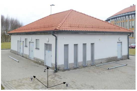
Figure 1.
The test object in the defined coordinate system.
In all possible combinations, the multiple measurements of the geodetic and photogrammetric network points were performed using Leica TS30 total station (angle horizontal Hz/vertical V measurement accuracy 0.5″, pinpoint EDM precise accuracy 0.6 mm + 1 ppm to a prism) in the global object coordinate system. The spatial geodetic control network of 12 stabilized ground points by iterative multi-observation parametric adjustment was carried out. In practice, the task was realized with the model of observation equations:
where K is the direction to the unknown point, V is the residual, Az is the azimuth, and Z is the station orientation constant. Equation (1) is linearized by Taylor series expansion:
and bearing coefficients:
Variation function φ based on Equation (2) is derived using a direct approach and is obtained by the least squares criterion: , and is given as:
where (P) is the weight matrix , A is the matrix of the partial derivatives of the parametric equations, L is the misclosure vector, X—unknown. The resulting equation after finding the partial derivatives of the variation function is:
Using basic matrix algebra, the least squares normal equation system is given:
The solution from the normal equation system is solved as follows:
The solution of the elevation network is realized by the parametric model where are the adjusted observations and are the unknown parameters . The parametric equations are formulated as follows:
where HI is the measured distance between a horizontal line of sight of the total station instrument and point i, HT is the distance between the target and point j, is the slope distance between points ij, is the measured zenith angle, and is the height difference between points ij.
The design matrix A is given as partial derivatives of parametric equations . The formed misclosure vector L was realized by substituting the approximate values of point elevation and original observations l:
The weight matrix (P) of elevation differences is given:
where and s is the standard deviation. The solution of vector X is described in Equation (6). The parameters used and obtained during adjustment are presented in Table 1.

Table 1.
Control network adjustment parameters.
The coordinates of the photogrammetric control network (targets) were computed using the multiple spatial angular–linear intersections (see Figure 2).
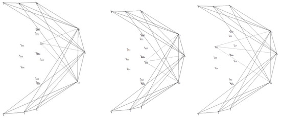
Figure 2.
An example of photogrammetric control network measurement schema (multiple spatial angular-linear intersections for points 407, 408, 453).
For image acquisition, the DSLR Nikon D5100 camera, equipped with the CMOS sensor (23.6 × 15.6 mm size, resolution 4928 × 3264, the pixel size p’xy = 4.78 µm) and the lens with optical stabilization (the zoom lens f = 18 ÷ 55 mm), focused (focal f = 18 mm) on the imaging distance approx. YI = 10.0 m (GSD ≅ 3 mm) was used. A total of 104 terrestrial, mainly convergent photos were taken from elevated camera standpoints. The maximum enhancement of the base/distance ratio υ and the longitudinal overlap enhanced the geometry of the photos block. Depending on the local imaging scale, the diameter of targeted control and check points on the images varied between 5÷15 pixels.
In the datasets adopted for digital processing and 3D reconstruction, only 36 images (see CRBeDaSet_Images.pdf file of the CRBeDaSet online repository) were included, the best ones in geometric and radiometric quality aspects from a photogrammetric point of view. The block of 28 photos for analytical bundle adjustment was applied.
3.2. Bundle Adjustment and Camera Calibration
In order to determine the additional check points for the study of the geometric accuracy of the 3D models and to create the benchmark data set, the digital image measurements and combined bundle block adjustment with simultaneous camera calibration in the Pictran software package were performed. The simultaneous on-the-job calibration method most accurately corresponds to the real conditions of image acquisition and provides the optimal functional model of the solution by bundle method.
The initial camera calibration model was included. It contains basic elements of the interior orientation cK, x’0, y’0, and additional parameters modeling the systematic lens errors: radial symmetric distortion A1 and A2, tangential (decentering) distortion B1 and B2, and affinity C1 and shear error C2 of the digital sensor array (Table 2).
Table 2.
Calibration parameters of the DSLR Nikon D5100 camera.
The control points were applied to the adjustment as observations with errors (weighted). The a priori estimated accuracy of signalized points was SXYZ = 1 mm, whereas natural points of SXYZ = 3 mm. The elements of spatial orientation of all photos were unavailable (not observed) and were not added as estimated observations to the adjustment. The bundle block adjustment conditions were: number of observations—1995 and number of unknowns—1039. In the automatic elimination of errors, the parameters were: normalized residual termination—0.4000 × 10, and the maximum number of data-snooping—5.
The spatial coordinates of the 24 photogrammetrically-computed new points (photogrammetric new check points) were obtained with mean standard deviations of SX = 0.84 mm, SY = 0.83 mm, and SZ = 0.61 mm, respectively. The configuration of convergent photos has ensured the homogeneous accuracy of the calculated point coordinates. The results of the optimal variant of the adjustment were used for further digital processing and analyses.
3.3. Terrestrial Laser Scanning
For the acquisition of ground truth information and accuracy comparison purposes, the test object CRBeDaSet was scanned using the Leica ScanStation C10. It is a compact, pulsed, dual-axis compensated, high-speed laser scanner. The accuracy parameters of a single measurement at 1 ÷ 50 m range (one sigma) are: position—6 mm, distance—4 mm, angle Hz/V—12″, modeled surface precision/noise—2 m, and target acquisition—2 mm standard deviation.
The four scan stations were located in the distance YS ≈ 10.0 m from each elevation. A single scan was performed in the local coordinates system with a maximal resolution of 1 mm (Figure 3 shows the density of the TLS point cloud). For scan fusion, 8 HDS scan targets were applied. Figure 4a shows the scanned test object CRBeDaSet with the position of 4 scan stations and 8 HDS scan targets.
Figure 3.
TLS point cloud density.
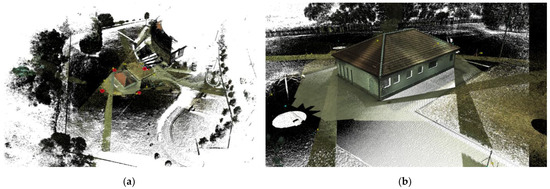
Figure 4.
Colored point cloud obtained from merged 4 TLS scans. (a) Test object CRBeDaSet with the position of 4 scan stations and 8 HDS scan targets. (b) The detailed view on the main test object.
The point clouds merging fusion and data processing were carried out in the Leica Cyclone™ SCAN software. The global filtered point cloud for the test object CRBeDaSet consisted of ca. 250 million points (17.2 GB saved in *.pts file). The Leica ScanStation C10 is equipped with an auto-adjusting, integrated digital camera with a zoom video. In the project, each point was matched with the pixel color of a digital image. The visualization of the point cloud is presented in Figure 4a,b.
Then, the point cloud was manually denoised. All points which were acquired on humans, cars, and other objects in the move were removed. Additionally, points that represent the interior of the building (measured through the holes, windows, or glass) were removed. After that, to change the density of the points, the point cloud was filtered using the minimum space between points. The raw space between points (0.0001 m) was changed to 0.003 m, as it is enough to recognize even small objects, and the point cloud is not too large for machine and deep learning purposes. In the last step, the point cloud of the main object (building) and its surroundings were manually classified using the LoD3 standard, and 18 classes were specified. Semantic segmentation was performed in the pointly.ai web app. Due to this and the numbers of the classes being related to the ASPRS *.las format (http://www.asprs.org/wp-content/uploads/2019/03/LAS_1_4_r14.pdf, accessed on 22 April 2022) which also contains classes reserved for ASPRS definitions, the respective classes were used in this study:
- 0—unclassified (this class is empty, but in many machines and deep learning models, it is defined as not used),
- 2—ground (in this class, the bare ground is included),
- 3—low vegetation (this class contains grass and other vegetation which was mowed),
- 4—medium vegetation (this class is related to the bushes, shrubs, and plants which are not trees),
- 5—high vegetation (this class contains the whole trees: trunks, branches, and leaves)
- 12—paved terrains (because of the same material, which was used to prepare the sidewalks, roads, and parking lots, they were merged into one class),
- 19—building façades (the exterior walls of buildings—from ground to the roof, excluding windows, sills, doors, vents, drainpipes, and technical infrastructure localized on building walls),
- 20—tiles (building roofs and elements above roofs were divided into three classes. The tile class shows the material of the external cover (roofing),
- 21—roof construction (this is the second class of roof elements, which contains all roof parts which cannot be bracketed together with tiles, e.g., wooden and steel eaves, steel construction elements),
- 22—windows (the points which show the plane of the windows (window frames) are included; both windowpane and glass bricks planes are contained in this class),
- 23—vehicles (parked vehicles are included in this class; the points which belong to vehicles in the move were filtered out before classification),
- 24—drainpipe (this class contains all elements of rain infrastructure localized on the buildings, including, e.g., drainpipes, rain gutters, downspouts, branches, and socket bends),
- 25—sill (this class contains all points registered on window sills, including different materials from which they were designed, e.g., steel, PVC, aluminum),
- 26—doors and vents (door and vents were accumulated into one class because the main test object is an electric room building where some parts of doors are very similar or even identical to steel vents, e.g., see Figure 1),
- 27—urban furniture (in this class, all points registered on infrastructure signs, e.g., safety, construction, and property signs; fence; snow fence for roof tiles; sidewalk barriers, entrance gate, and carpet hanger are included),
- 28—technical infrastructure (this class contains all technical infrastructure that belongs to the buildings and their environments, including street and external building lamps, electric boxes, manholes, and other technical items),
- 29—surveying equipment (all points registered on surveying equipment like TLS targets, surveying poles, and bipods),
- 30—chimney (this class contains chimney and chimney pot).
Due to the high number of points and the web app user interaction processing possibilities, the semantic segmentation process was verified and corrected in Arena4D software (ver. 9.5.0.13890). The final product has ca. 62 million points classified into 18 classes and is presented in Figure 5. The point distribution in 18 classes is presented in Figure 6. Due to the special case study of a low-rise building, class 20 (tiles) in the typical city scene might be overrepresented. It is recommended that the proposed data should be adapted to the semantic segmentation scenario by class weighting.
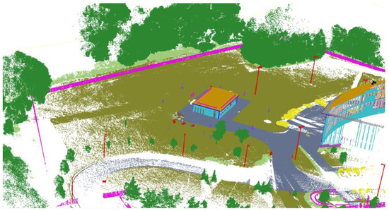
Figure 5.
The overview of the manually classified TLS point cloud.
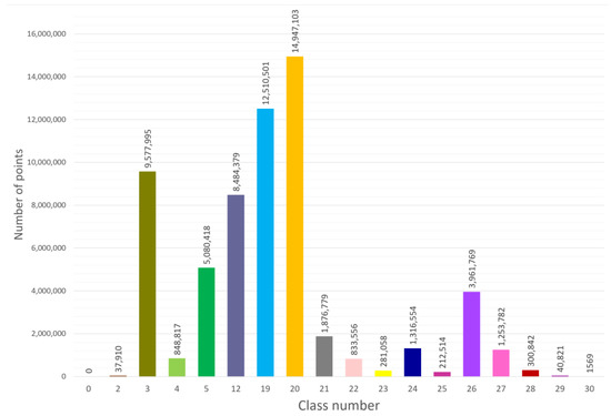
Figure 6.
The distribution of different semantic classes in our CRBeDaSet. Note that a small number of points are annotated as class 30 due to only having one chimney. Additionally, note that authors do not divide the dataset into train and test parts. Because of that, users may decide which objects are needed (delete not necessary objects) for the research and then cut parts of the object for validation and test purposes.
4. CRBeDaSet—Test and Analysis
The presented experiment scenario was designed to prepare the assessment of quality and geometric accuracy of a medium-size building 3D reconstruction based on photogrammetric, multi-image view, uncalibrated imagery. The second aspect of this dataset was to allow researchers to objectively compare the accuracy, functionality, and reliability of photogrammetric applications for 3D object reconstruction. Our test and analysis were divided into three stages:
- The tests of the CRBeDaSet in applications dedicated to 3D object modeling and reconstruction.
- The accuracy analysis of the image-based and TLS point clouds.
- The evaluation of detectors and descriptors on the object with a homogenous structure.
4.1. Dataset Processing
For verification of the dataset, we used one open-source application: inteGRAted PHOtogrammetric Suite (GRAPHOS, ver. 1.0.35) and four well-known and very popular commercial suites: ContextCapture (ver. 10.19.00.122), Metashape (ver. 1.8.4.14856 and PhotoScan ver. 1.4.5.7354), Pix4Dmapper (ver. 4.7.5), and RealityCapture (ver. 1.2.1.116295). Due to changes in the computation algorithms in Agisoft software (ver. 1.5.0), both versions (Metashape and PhotoScan) were included in the tests. The workflow for this stage of analysis is presented in Figure 7.
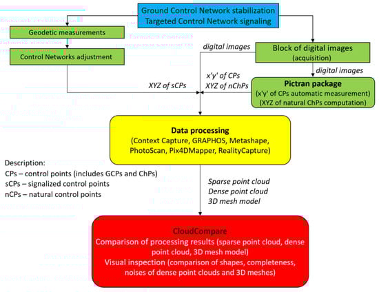
Figure 7.
The workflow for CRBeDaSet tests in different applications dedicated to 3D object modeling and reconstruction.
The digital processing in the tested software was performed using preprepared batch files to prepare a similar computation environment. These files contain image pixel coordinates of all points measured automatically in the external Pictran DE software (ver. 4.3) and photogrammetric control network (artificially signalized and natural points) ground coordinates. All computations were performed with minimal user participation with similar and possible-to-use computing parameters. The results of three computation stages (image-matching, densification, and meshing) were compared using visualizations and descriptions (in the form of tables) to show computation differences. The results of the image matching stage and BBA of CRBeDaSet processing in five applications dedicated to photogrammetric purposes are presented in Figure 8. While in the case of ContextCapture and PhotoScan, most of the tie points are localized on the main object, in the case of Pix4DMapper and RealityCapture, many tie points are background points (visible noise) containing grass, shrubs, trees, cars, and steel-glass elevation of the second building, which is also visible on GRAPHOS and Metashape results.
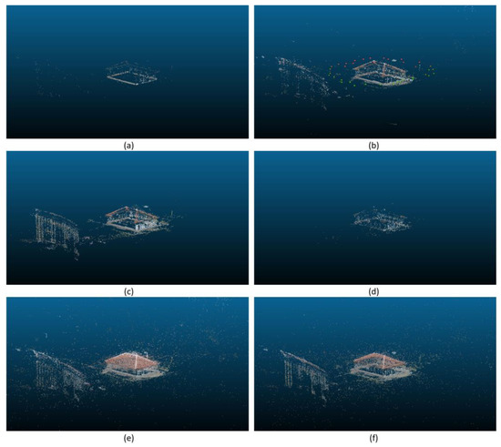
Figure 8.
Sparse point clouds generated in: (a) ContextCapture; (b) GRAPHOS; (c) Metashape; (d) PhotoScan; (e) Pix4DMapper; (f) RealityCapture.
Figure 9 shows the results of point cloud densification (based on the ContextCapture example). The first image shows the general look of the reconstructed region. The next images present detailed views on roof and façade geometry and point distribution.
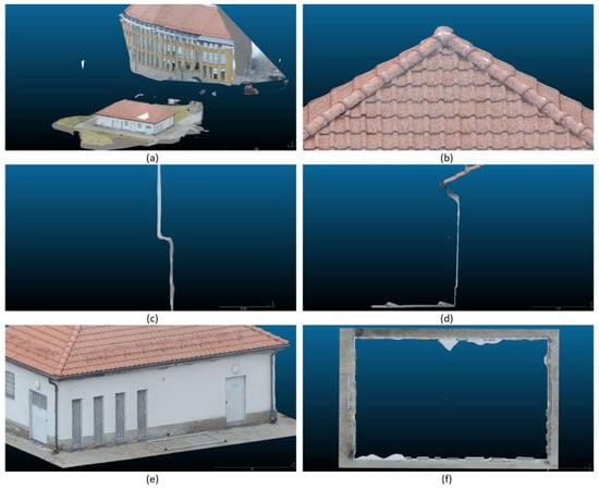
Figure 9.
ContextCapture dense point cloud: (a) general look on generated point cloud; (b) roof geometry reconstruction; (c) place where clinker tiles contact wall without visible texture; (d) vertical section of elevation 1; (e) closer look at the corner of the building; (f) top view on the building without a roof.
The comparison of all software results is presented in Figure A1 (Appendix A). The fulfillment of the points in the reconstructed region (presented in row 1) is different, from dense point clouds with visible holes (GRAPHOS case) to fully covered objects (ContextCapture case). Pix4DMapper results look unusual—all regions without visible texture were not reconstructed in the densification step using high resolution (it is also possible to obtain these regions by using the user’s dedicated parameters). The roof reconstruction shows how the application can handle the sky registered on images and how such points are filtered in the final product. Rows 3 and 4 show how applications reconstruct places where the intersection of two planes occurs if the corners are rounded or present a proper 90-degree shape and how much noise is generated. Row 5 deals with the connection between different elevation objects and shows how not fully visible objects are reconstructed (based on snow fences for roof tiles). The last row (6) presents what the geometry of reconstructed walls is (including places without visible texture).
Figure 10 shows the results of mesh model generation (based on the ContextCapture example). The detailed comparison of the results from used application is presented in Figure A2 (Appendix A). Due to the fact that GRAPHOS does not have a built-in feature to generate mesh geometry, it is not included in the collation. All generated mesh 3D models filled up holes presented on dense point clouds. In the case of Metashape, PhotoScan, and Pix4DMapper, some visible parts of the sky on the roof which were not filtered occurred. On all models, the clinker tiles’ shape and wall texture are visible; however, in the case of Metashape and PhotoScan, the microporous geometry of the mesh model is visible. The place where roof and wall planes meet is generating issues in every application, from a slight rounding of the corner (ContextCapture, RealityCapture) through some noise production (PhotoScan) and generation of extrapolated geometry (Metashape and Pix4DMapper). The Pix4DMapper fulfilled holes in walls without the visible texture of the mesh model; however, because of the variation of Poisson surface reconstruction algorithm [91], they are not straight, but rounded. Avoiding such issues (using planar constraints) is possible, but it requires the user’s manual interference. The geometry of walls show that the ContextCapture issue related to the wrong reconstruction of bigger parts of the wall without visible texture (extrapolating objects—cleating craters on walls in the direction to inside the building) is not filtered out during mesh model computation. Due to the good texture of the mesh model, the geometry imperfections appear to be hidden in other visual presentations.
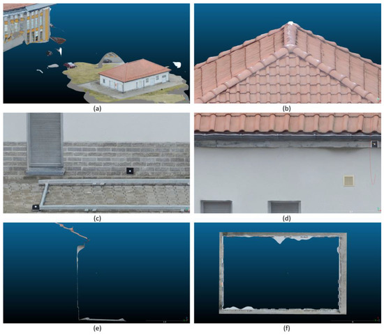
Figure 10.
ContextCapture 3D mesh model: (a) general look on generated mesh 3D model; (b) roof geometry reconstruction; (c) façade with clinker tiles and wall without visible texture; (d) corners of the building roof and wall without visible texture; (e) vertical section of elevation 1; (f) top view on the building without a roof.
The summary of the generated products is presented in Table 3. As the computations were performed on two workstations (laptop MSI Titan GT77 12UHS and desktop described in [56]), the computation time is not compared.
Table 3.
Characteristics of generated products in used software.
4.2. Accuracy Analysis of CRBeDaSet Digital Processing
The analytical study on the geometric accuracy of the generated image-based point clouds includes the analysis of deviations (coordinates differences) between the control point coordinates of the photogrammetric network, measured directly by means of the Leica TS30 total station (the input dataset) and the results (the final software log files) of digital processing and bundle adjustment using the tested software. The geometric analysis workflow is presented in Figure 11.
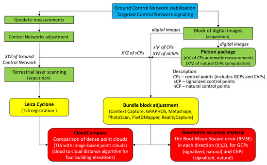
Figure 11.
The workflow for image-based and TLS point clouds accuracy analysis.
The summary of bundle block adjustment computed in tested software is performed by the comparison of the RMS values on GCPs (presented in Table 4) and ChPs (presented in Table 5), considering targeted and natural points separately and together.
Table 4.
The RMSE values on GCPs obtained in tested software after BBA.
Table 5.
The ChPs RMS values obtained in tested software after BBA.
The tested COTS software allowed point matching on all control points with the subpixel accuracy—the mean standard deviation sx’y’ < 0.50 pixel was obtained. The average root mean square errors on control points RMSE (XYZ) GCPs = 3 mm and check points RMSE (XYZ) ChPs < 3 mm were determined, which is equivalent to a relative accuracy of ca. 1/6600 in object space. Considering the applied functional model of digital processing, the obtained results can be accepted as sufficient. In the case of the GRAPHOS suite, the obtained results were higher. It is related to the computation chain because the coordinates of GCPs and ChPs are used in BBA after matching and camera calibration procedures to scale the model. While in the COTS software it is possible to compute the whole model based on provided GCPs and ChPs, in the GRAPHOS suite, their influence on the model is less, and correct automatic tie points must be computed.
In the second part of the geometric analysis, TLS point cloud was used. The root mean square errors obtained in the Leica Cyclone application during the registration using targeted points localized on the geodetic control network were the following: RMSE(X) = 2.0 mm, RMSE(Y) = 3.8 mm, and RMSE(Z) = 1.8 mm. The accuracy of the TLS point cloud was also evaluated using manual measurements of signalized photogrammetric control network points centers and natural ChPs localized in the corners of ventilation niches and doorways (measured using elevation planes cut from the point cloud, see Figure 12a). Figure 12b shows how the signalized targets were registered in TLS point cloud, and Table 6 contains the RMSE values for measured points.
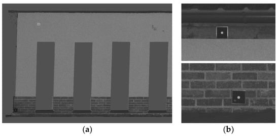
Figure 12.
The measurements of sCPs and nChPs on TLS point cloud: (a) elevation plane cut from the model for nChPs measurements; (b) sCPs visualization on TLS point cloud.
Table 6.
The analysis of manual measurements of sCPs and nChPs on TLS point cloud.
While TLS scan stations were registered with high density, which was very time-consuming, it may be observed that one target used for merging scans moved and influenced the elevation 2. The target was eliminated from registration; however, the merged point cloud had bigger registration errors on the elevation 2 (E2) scan. Due to that, the target measurements were divided into two groups with elevation two and without. Considering the manual measurement error and TLS point cloud density, the obtained RMSE values on sCPs and nChPs (excluding E2) are acceptable for geometric analysis purposes.
Then, the obtained image-based point clouds were compared to the TLS point cloud using the cloud-to-cloud distance algorithm [47,92,93]. Figure 13 shows the obtained differences for ContextCapture, and the comparison of tested software outputs is included in Figure A3, Figure A4, Figure A5, Figure A6 and Figure A7 (Appendix A).
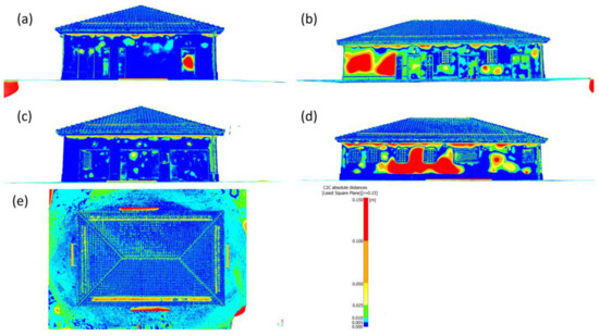
Figure 13.
The comparison between TLS and image-based point cloud (ContextCapture): (a) elevation 1; (b) elevation 2; (c) elevation 3; (d) elevation 4; (e) top view on the study area.
Because additional structures with signalized ground control points were used for image acquisition, on all comparisons with the TLS point cloud, these objects (localized near the building) are signalized as a gross error. Elevation 2 shows distances between point clouds which are similar to the TLS registration error. Because of the shape and size, the snow fence for roof tiles is reconstructed with errors in all applications. Additionally, the shape of the roof tiles creates different issues in reconstruction. In all applications, the drainpipes’ correct shape is an issue; however, the errors in the areas near vertical drainpipes are mainly caused by laser-beam slipping. In the case of ContextCapture, the results showed large deformations in bigger parts of the façade where no visible structure is localized. The places where walls stitch with the roof (90-degree corners) look rounded. The repeated shape of the ventilation grate showed reconstruction errors below 25 mm. The GRAPHOS case shows issues related to the side parts of the façades. While in the center parts, distances to TLS are below 5 mm, on the sides, they rise to more than 50 mm in the case of elevation 3 and 25 mm for elevation 4. Analyzing Metashape and PhotoScan, the noise filtering should be pointed out. It is visible that some efforts were made to cut off the points, which are reconstructed using images where clouds are registered near the roof. Still, there are some issues with rounding corners, which are mainly visible on elevation 4. The Pix4DMapper case shows that the neighborhood of the building is more deformed than in other applications, but it is below 25 mm. Due to the reconstruction being limited to the visible features and shapes of the façade, the deformation of glass brick windows has not occurred. Some changes are visible on ventilation grates, i.e., elevation 1 (errors below 25 mm) and 3 (errors rise to more than 100 mm). The roof of the building consists of slightly higher deformations than in other applications. The RealityCapture case shows good performance on walls without visible features and roof structure; however, ventilation grates and glass brick windows showed deformations below 50 mm (elevation 4).
4.3. Evaluation of Detectors and Descriptors on CRBeDaSet
While the microporous texture could be recognized in the terrain, the image registration shows that it should be treated as a surface without visible texture for matching purposes. Due to that, the third part of the evaluation is related to different detectors and descriptors. Tests were performed for four elevations (two more extended and two shorter) which contain different characteristics. The selection of images on which the tests were carried out was related to the simulation of real measurement conditions in which 100% longitudinal overlap does not occur. The workflow for this part of the study is presented in Figure 14.
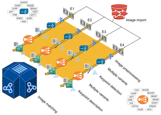
Figure 14.
Image matching evaluation workflow.
In case 1, the surface of the wall of elevation 1 (E1) without visible texture is limited by four big rectangular ventilation grates with repeated shapes, a door with a small information board, drain pipes, and some small objects (technical infrastructure) with visible shapes. The down part of the façade is covered by clinker tiles. Besides, on the images are registered ceramic roof tiles (repeated shape), snow fences for roof tiles, paved terrain, trees, and technical infrastructure. The second elevation (E2) contains less wall surface without texture than E1 and includes more doors with information boards, more small technical infrastructure, and two glass brick windows. The third elevation (E3) has many objects with visible shapes, i.e., three double doors with information boards and rectangular ventilation grates (down and central part of doors), a big rectangular ventilation grate near doors, and technical infrastructure. The wall surface without visible texture is very limited. The fourth elevation (E4) includes four glass block windows and two windows with closed built-in roller shutters and more technical infrastructure, as well as more surface without visible texture. The tests were performed using 12 detectors and 14 descriptors (all to all method) using the GRAPHOS suite [7], PhotoMatch software [19], and our own implementation of Python.
The results of different detectors are presented in Figure A8 and Tables S1–S4 of supplementary files (for four elevations), while a short description is presented in Table A1, Table A2, Table A3 and Table A4. The images in high resolution are included in the CRBeDaSet_tests online repository.
The outcome of the different detectors and descriptors was divided into three groups based on the number of errors during the matching. The groups were defined as follows (Equation (10)):
where is number of matched points, is number of wrongly matched points, and is a matching result. The results of matching tests are presented in Table S5 of the supplementary file in the form of images with marked points and in the form of tables (Table A1, Table A2, Table A3 and Table A4 of Appendix B) using the description from Equation (10). Furthermore, the detection and description time, number of keypoints, and number of matched points for short (E3) and long (E4) elevations are presented in Tables S6–S7 of the supplementary file. Based on the division of matching results from four elevations (Table A1, Table A2, Table A3 and Table A4 of Appendix B), the analysis showed which descriptors and detectors might be used in the case of buildings with large parts of walls with no visible features (Table 7).
Table 7.
The results of matching performed for four elevations. The description is performed according to Equation (10), and the “*” symbol means a descriptor not available, and the places where the “xxxx” symbol appears mean different results for different elevations. The abbreviations of detectors and descriptors are used as they were proposed by authors of these algorithms.
Furthermore, based on the number of matches, the detectors (including all used descriptors for which the matching result is positive) might be classified into three main groups:
- Below 20 matched points (GFTT, MSD, ORB, SIFT, STAR).
- Between 20 and 100 matched points (BRISK, KAZE).
- Under 100 matched points (AGAST, SURF).
In the case of FAST, AKAZE, the results depend on the object features registered on images and due to that, both are between groups 2 and 3. The MSER detector is classified between groups 1 and 2. While for group 3, most of the points are localized on clinker bricks, for group 1, points are mainly localized on information boards, corners of ventilation, and window and door niches. An interesting case is the MSD detector with VGG and SIFT descriptors, which show matched points mainly near artificially signalized ground control points. Considering descriptors, the case of BOOST shows a visible smaller number of matched points, and usage of the LSS is the most time-consuming.
5. Discussion
A new CRBeDaSet benchmark dataset is presented for evaluating image-based 3D modeling and reconstruction techniques. The high-accuracy survey measurement instruments, as well as geodetic and photogrammetric professional software, were used to prepare the analytical data of the CRBeDaSet because only high-quality and accurately-input data provides a reliable evaluation of the algorithms and applications’ quality.
The first practical experiences of using the CRBeDaSet to assess the accuracy and reliability of tested applications (ContextCapture, GRAPHOS, Metashape, PhotoScan, Pix4Dmapper, and RealityCapture) confirmed the usefulness of the prepared real data. The CRBeDaSet has a number of characteristics that can support the development of new approaches to the high-accuracy 3D reconstruction of medium sized objects (object shape with a volume ca 1000 m3) in close range. The development of applications dedicated to photogrammetric reconstruction is still in high demand. Based on the presented results and previous works [26], it can be seen that developers in recent years put some effort into noise filtering, smoothing of the reconstructed surfaces, and computation time. Still, some computation errors might occur during the matching part, which could be caused by imperfections of software, e.g., the ineffectiveness of algorithms or their incorrect implementation.
Due to the presented test object in CRBeDaSet being composed of paving, walls covered partially with bricks, multiplicated objects with sharp shapes (ventilation grates), and homogenous texture of a wall and roofing tiles, there should be enough features to process the data. However, during the processing of the presented dataset, the following difficulties occurred:
- Faulty matching of tie points is related to a brute force approach where all possible image pairs are evaluated (Figure 15a).
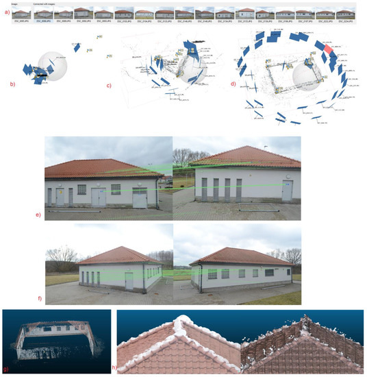 Figure 15. Software problems in processing the CRBeDaSet: (a) faulty matching of tie points; (b–d) the examples of the problems with optimal selection of tie points and weight assignment; matching problems related to (e) repeated regular shapes and color of roofing tiles and (f) localization of windows and vent holes near homogenous texture of wall; (g) shortages in point clouds; (h) difficulty with correct automatic filtering of dense point clouds during the mesh generation.
 - Problems with the optimal selection of tie points and weight assignment in the adjustment process (Figure 15b–d).
- Shortages in point clouds (Figure 15g) and mesh discontinuities on projection distorted regular parts of the roof.
- Some of the tested software has difficulty with the correct automatic filtering of dense point clouds during the mesh generation (Figure 15h).
The first three errors could be resolved by using different matching algorithms, and due to that, we have prepared a comparison of the detectors and descriptors. Based on the tables (Table A1, Table A2, Table A3, Table A4 and Table S6) and images (Tables S1–S5), it is possible to choose algorithms that cover developers’ assumptions. The process deals with a large number of tie points which might result in errors, as presented in Figure 15b–d), or a limited number of tie points to acquire shorter computation time with a smaller number of matches. In our study, to perform tests without manual tuning of detectors’ and descriptors’ parameters (i.e., feature number, octave layers, thresholds), the standard values were used. By tuning these factors, different results might be obtained.
The second part of the dataset is related to TLS point cloud registration and semantic segmentation of point clouds. The presented CRBeDaset contains a complex photogrammetric control network, which might also be used for scan station registration. In recent years, the topic of TLS point clouds registration has been explored, and according to Li et al. [94], there are three ways to increase the accuracy of the computation. Firstly, by improving filtering algorithms; secondly, by developing or enhancing feature descriptors; and thirdly, by making progress in 3D surface matching. Our CRBeDaSet allows scientists to work with the first two mentioned ways, and already-performed computations might be used as a reference. Based on our proposed dataset, other researchers might train their machine learning algorithms (i.e., self-organizing maps or K-means) to filter noisy point clouds and reach better accuracy of the final 3D model [95], which is very important, especially in cultural heritage studies.
Furthermore, in the second part of our dataset, the LoD3 classification topology of the 3D outdoor point cloud was used. It is important for future development of the semantic segmentation algorithms because the indoor scenes in LoD3 class topology are available; however, there is a deficit of outdoor scene availability.
The dataset can be accessed via the DOI repository website, CRBeDaSet: http://dx.doi.org/10.17632/9nvn27yw62.2 (images, coordinates, and raw merged TLS point cloud) and CRBeDaSet_tests: http://dx.doi.org/10.5281/zenodo.7496481 (raw scan stations, filtered point cloud in control network coordinate systems, annotated point clouds, high-resolution images, analyses of point clouds obtained using COTS software, TLS to image-based point cloud distance results, and matching parts).
Future investigations will be focused on developing and increasing the CRBeDaSet by dedicating scenarios for the highest geometric accuracy 3D object reconstruction using precise geodesy surveying for control networks and direct georeferencing, multi-view terrestrial and UAV imagery, corridor mapping on GPS-denied areas, and, additionally, more TLS scan stations.
Supplementary Materials
The following supporting information can be downloaded at: https://www.mdpi.com/article/10.3390/rs15041116/s1, Table S1: The results of using different detectors in the E1 images; Table S2: The results of using different detectors in the E2 images; Table S3: The results of using different detectors in the E3 images; Table S4: The results of using different detectors in the E4 images; Table S5: The image matching results of elevation 1–4 using different detectors and descriptors; Table S6: The results of image matching for shorter elevation; Table S7: The results of image matching for longer elevation.
Author Contributions
Conceptualization, G.G. and P.S.; methodology, G.G.; software, G.G. and P.S; validation, G.G.; formal analysis, G.G.; investigation, G.G.; resources, G.G. and P.S; data curation, G.G. and P.S; writing—original draft preparation, G.G.; writing—review and editing, G.G. and P.S; visualization, G.G.; supervision, P.S.; funding acquisition, G.G. All authors have read and agreed to the published version of the manuscript.
Funding
This research was partially funded by the Polish National Agency for Academic Exchange (NAWA), grant number BPN/BEK/2021/1/00246/U/00001, and the APC was covered by the G.G.
Data Availability Statement
While the data presented in this study are openly available in CRBeDaSet at http://dx.doi.org/10.17632/9nvn27yw62.2, the test part of the data will be available in CRBeDaSet_tests at http://dx.doi.org/10.5281/zenodo.7496481 from the date of publication.
Acknowledgments
We thank Andrzej Dumalski for his technical support with TLS data acquisition. Additionally, we thank Veesus company for the possibility of using their software (Arena4D) for research purposes.
Conflicts of Interest
The authors declare no conflict of interest.
Appendix A. The Results of the CRBeDaSet Processing


Figure A1.
Comparison of the dense point clouds generated in used software: (a) ContextCapture; (b) GRAPHOS; (c) Metashape; (d) PhotoScan; (e) Pix4DMapper; (f) RealityCapture.
Figure A1.
Comparison of the dense point clouds generated in used software: (a) ContextCapture; (b) GRAPHOS; (c) Metashape; (d) PhotoScan; (e) Pix4DMapper; (f) RealityCapture.


Figure A2.
Comparison of the 3D mesh models generated in used software: (a) ContextCapture; (b) Metashape; (c) PhotoScan; (d) Pix4DMapper; (e) RealityCapture.
Figure A2.
Comparison of the 3D mesh models generated in used software: (a) ContextCapture; (b) Metashape; (c) PhotoScan; (d) Pix4DMapper; (e) RealityCapture.


Figure A3.
Comparison of TLS and image-based point clouds of elevation 1: (a) ContextCapture; (b) GRAPHOS; (c) Metashape; (d) PhotoScan; (e) Pix4DMapper; (f) RealityCapture.
Figure A3.
Comparison of TLS and image-based point clouds of elevation 1: (a) ContextCapture; (b) GRAPHOS; (c) Metashape; (d) PhotoScan; (e) Pix4DMapper; (f) RealityCapture.


Figure A4.
Comparison of TLS and image-based point clouds of elevation 2: (a) ContextCapture; (b) GRAPHOS; (c) Metashape; (d) PhotoScan; (e) Pix4DMapper; (f) RealityCapture.
Figure A4.
Comparison of TLS and image-based point clouds of elevation 2: (a) ContextCapture; (b) GRAPHOS; (c) Metashape; (d) PhotoScan; (e) Pix4DMapper; (f) RealityCapture.


Figure A5.
Comparison of TLS and image-based point clouds of elevation 3: (a) ContextCapture; (b) GRAPHOS; (c) Metashape; (d) PhotoScan; (e) Pix4DMapper; (f) RealityCapture.
Figure A5.
Comparison of TLS and image-based point clouds of elevation 3: (a) ContextCapture; (b) GRAPHOS; (c) Metashape; (d) PhotoScan; (e) Pix4DMapper; (f) RealityCapture.


Figure A6.
Comparison of TLS and image-based point clouds of elevation 4: (a) ContextCapture; (b) GRAPHOS; (c) Metashape; (d) PhotoScan; (e) Pix4DMapper; (f) RealityCapture.
Figure A6.
Comparison of TLS and image-based point clouds of elevation 4: (a) ContextCapture; (b) GRAPHOS; (c) Metashape; (d) PhotoScan; (e) Pix4DMapper; (f) RealityCapture.


Figure A7.
Comparison of TLS and image-based point clouds of the test object (top view): (a) ContextCapture; (b) GRAPHOS; (c) Metashape; (d) PhotoScan; (e) Pix4DMapper; (f) RealityCapture.
Figure A7.
Comparison of TLS and image-based point clouds of the test object (top view): (a) ContextCapture; (b) GRAPHOS; (c) Metashape; (d) PhotoScan; (e) Pix4DMapper; (f) RealityCapture.

Appendix B. The Results of Image Matching Using Different Detectors and Descriptors

Figure A8.
Differences between keypoints detection using tested detectors for one image of CRBeDaSet. The presentations of keypoint detection for four elevations (4 × 2 images) are included in supplementary files.
Figure A8.
Differences between keypoints detection using tested detectors for one image of CRBeDaSet. The presentations of keypoint detection for four elevations (4 × 2 images) are included in supplementary files.

Table A1.
The results of matching performed for elevation 1. The description is performed according to Equation (10), and the “*” symbol means descriptor not available.
Table A1.
The results of matching performed for elevation 1. The description is performed according to Equation (10), and the “*” symbol means descriptor not available.
| Detectors | E1 | ||||||||||||
|---|---|---|---|---|---|---|---|---|---|---|---|---|---|
| Descriptors | AGAST | AKAZE | BRISK | FAST | GFTT | KAZE | MSD | MSER | ORB | SIFT | STAR | SURF | |
| AKAZE | * | OK | * | * | * | OK | * | * | * | * | * | * | |
| BOOST | OK | H | ERR | OK | ERR | ERR | ERR | H | ERR | ERR | OK | OK | |
| BRIEF | OK | OK | OK | OK | OK | OK | ERR | OK | H | ERR | H | OK | |
| BRISK | OK | OK | OK | OK | OK | OK | ERR | OK | OK | H | H | OK | |
| DAISY | OK | OK | OK | OK | OK | OK | H | OK | OK | OK | OK | OK | |
| FREAK | OK | OK | OK | OK | OK | OK | ERR | OK | OK | ERR | ERR | OK | |
| HOG | ERR | ERR | * | ERR | ERR | ERR | H | OK | OK | ERR | ERR | OK | |
| KAZE | * | H | * | * | * | OK | * | * | * | * | * | * | |
| LATCH | OK | OK | OK | OK | OK | OK | H | H | OK | OK | OK | OK | |
| LSS | OK | OK | H | OK | OK | OK | H | OK | ERR | ERR | OK | OK | |
| ORB | OK | OK | OK | OK | OK | OK | ERR | OK | OK | * | OK | OK | |
| VGG | OK | OK | OK | OK | OK | OK | OK | OK | OK | OK | OK | OK | |
| SIFT | OK | OK | OK | OK | OK | OK | OK | OK | OK | OK | OK | OK | |
| SURF | OK | H | OK | OK | ERR | OK | ERR | OK | OK | ERR | ERR | OK | |
Table A2.
The results of matching performed for elevation 2. The description is performed according to Equation (10), and the “*” symbol means descriptor not available.
Table A2.
The results of matching performed for elevation 2. The description is performed according to Equation (10), and the “*” symbol means descriptor not available.
| Detectors | E2 | ||||||||||||
|---|---|---|---|---|---|---|---|---|---|---|---|---|---|
| Descriptors | AGAST | AKAZE | BRISK | FAST | GFTT | KAZE | MSD | MSER | ORB | SIFT | STAR | SURF | |
| AKAZE | * | OK | * | * | * | OK | * | * | * | * | * | * | |
| BOOST | H | H | H | OK | ERR | H | ERR | OK | ERR | ERR | OK | OK | |
| BRIEF | OK | OK | ERR | OK | OK | OK | H | ERR | OK | OK | OK | OK | |
| BRISK | OK | OK | OK | OK | OK | OK | ERR | OK | H | ERR | OK | OK | |
| DAISY | OK | OK | OK | OK | OK | OK | H | ERR | OK | OK | OK | OK | |
| FREAK | OK | OK | OK | OK | OK | OK | ERR | OK | OK | ERR | ERR | OK | |
| HOG | ERR | ERR | * | ERR | ERR | H | ERR | ERR | OK | ERR | ERR | OK | |
| KAZE | * | OK | * | * | * | OK | * | * | * | * | * | * | |
| LATCH | OK | OK | ERR | OK | OK | OK | ERR | ERR | OK | OK | OK | OK | |
| LSS | OK | OK | ERR | OK | ERR | OK | ERR | ERR | ERR | ERR | H | OK | |
| ORB | OK | OK | H | OK | OK | OK | ERR | ERR | OK | * | OK | OK | |
| VGG | OK | OK | OK | OK | OK | OK | OK | OK | OK | OK | OK | OK | |
| SIFT | OK | OK | OK | OK | OK | OK | OK | ERR | OK | OK | OK | OK | |
| SURF | OK | OK | OK | ERR | ERR | OK | ERR | OK | OK | ERR | ERR | OK | |
Table A3.
The results of matching performed for elevation 3. The description is performed according to Equation (10), and the “*” symbol means descriptor not available.
Table A3.
The results of matching performed for elevation 3. The description is performed according to Equation (10), and the “*” symbol means descriptor not available.
| Detectors | E3 | ||||||||||||
|---|---|---|---|---|---|---|---|---|---|---|---|---|---|
| Descriptors | AGAST | AKAZE | BRISK | FAST | GFTT | KAZE | MSD | MSER | ORB | SIFT | STAR | SURF | |
| AKAZE | * | OK | * | * | * | OK | * | * | * | * | * | * | |
| BOOST | ERR | H | OK | OK | OK | ERR | ERR | ERR | OK | ERR | ERR | OK | |
| BRIEF | OK | OK | OK | OK | OK | OK | ERR | H | OK | OK | OK | OK | |
| BRISK | OK | OK | OK | OK | OK | OK | ERR | OK | OK | OK | H | OK | |
| DAISY | OK | OK | OK | OK | OK | OK | H | ERR | OK | OK | OK | OK | |
| FREAK | OK | OK | OK | OK | OK | OK | ERR | OK | OK | OK | ERR | OK | |
| HOG | ERR | ERR | * | ERR | ERR | ERR | ERR | ERR | H | ERR | ERR | OK | |
| KAZE | * | OK | * | * | * | OK | * | * | * | * | * | * | |
| LATCH | OK | OK | OK | OK | OK | OK | ERR | ERR | OK | OK | OK | OK | |
| LSS | OK | OK | ERR | OK | H | OK | ERR | ERR | ERR | OK | H | OK | |
| ORB | OK | OK | OK | OK | OK | OK | ERR | OK | OK | * | OK | OK | |
| VGG | OK | OK | OK | OK | OK | OK | OK | H | OK | OK | OK | OK | |
| SIFT | OK | OK | OK | OK | OK | OK | OK | ERR | OK | OK | OK | OK | |
| SURF | ERR | OK | OK | OK | ERR | H | H | ERR | OK | ERR | ERR | OK | |
Table A4.
The results of matching performed for elevation 4. The description is performed according to Equation (10), and the “*” symbol means descriptor not available.
Table A4.
The results of matching performed for elevation 4. The description is performed according to Equation (10), and the “*” symbol means descriptor not available.
| Detectors | E4 | ||||||||||||
|---|---|---|---|---|---|---|---|---|---|---|---|---|---|
| Descriptors | AGAST | AKAZE | BRISK | FAST | GFTT | KAZE | MSD | MSER | ORB | SIFT | STAR | SURF | |
| AKAZE | * | OK | * | * | * | OK | * | * | * | * | * | * | |
| BOOST | OK | OK | OK | OK | ERR | OK | H | OK | OK | OK | OK | OK | |
| BRIEF | OK | OK | OK | OK | OK | OK | ERR | OK | OK | H | OK | OK | |
| BRISK | OK | OK | OK | OK | OK | OK | H | OK | OK | OK | OK | OK | |
| DAISY | OK | OK | OK | OK | H | OK | H | OK | OK | OK | OK | OK | |
| FREAK | OK | OK | OK | OK | OK | OK | H | OK | OK | H | H | OK | |
| HOG | OK | OK | * | OK | ERR | OK | ERR | OK | OK | ERR | ERR | OK | |
| KAZE | * | OK | * | * | * | OK | * | * | * | * | * | * | |
| LATCH | OK | OK | OK | OK | OK | OK | H | OK | OK | OK | OK | OK | |
| LSS | OK | OK | OK | OK | H | OK | OK | OK | H | OK | OK | OK | |
| ORB | OK | OK | OK | OK | OK | OK | ERR | OK | OK | * | OK | OK | |
| VGG | OK | OK | OK | OK | OK | OK | OK | OK | OK | OK | OK | OK | |
| SIFT | OK | OK | OK | OK | ERR | OK | OK | OK | OK | OK | OK | OK | |
| SURF | OK | OK | OK | OK | ERR | OK | ERR | OK | OK | H | H | OK | |
References
- Jazayeri, I.; Fraser, C.; Cronk, S. Automated 3D Object Reconstruction via Multi-Image Close-Range Photogrammetry. ISPRS Int. Arch. Photogramm. Remote Sens. Spat. Inf. Sci. 2010, 38, 305–310. [Google Scholar]
- Gaglione, S.; del Pizzo, S.; Troisi, S.; Angrisano, A. Position Accuracy Analysis of a Robust Vision-Based Navigation. ISPRS Int. Arch. Photogramm. Remote Sens. Spat. Inf. Sci. 2018, 42, 355–361. [Google Scholar] [CrossRef]
- Grussenmeyer, P.; Khalil, O. A Comparison of Photogrammetry Software Packages for the Documentation of Buildings. In Proceedings of the International Federation of Surveyors, Saint Julian’s, Malta, 18–21 September 2000. [Google Scholar]
- Jaud, M.; Passot, S.; le Bivic, R.; Delacourt, C.; Grandjean, P.; le Dantec, N. Assessing the Ac-curacy of High Resolution Digital Surface Models Computed by PhotoScan® and MicMac® in Sub-Optimal Survey Conditions. Remote Sens. 2016, 8, 465. [Google Scholar] [CrossRef]
- Remondino, F.; Nocerino, E.; Toschi, I.; Menna, F. A Critical Review of Automated Photo-grammetric Processing of Large Datasets. ISPRS Int. Arch. Photogramm. Remote Sens. Spat. Inf. Sci. 2017, 42, 591–599. [Google Scholar] [CrossRef]
- Schöning, J.; Heidemann, G. Evaluation of Multi-View 3D Reconstruction Software. In Proceedings of the Computer Analysis of Images and Patterns; Azzopardi, G., Petkov, N., Eds.; Springer International Publishing: Cham, Switzerland, 2015; pp. 450–461. [Google Scholar]
- Gonzalez-Aguilera, D.; López-Fernández, L.; Rodriguez-Gonzalvez, P.; Hernandez-Lopez, D.; Guerrero, D.; Remondino, F.; Menna, F.; Nocerino, E.; Toschi, I.; Ballabeni, A.; et al. GRAPHOS—Open-Source Software for Photogrammetric Applications. Photogramm. Rec. 2018, 33, 11–29. [Google Scholar] [CrossRef]
- Giuliano, M.G. Cultural Heritage: An Example of Graphical Documentation with Automated Photogrammetric Systems. ISPRS Int. Arch. Photogramm. Remote Sens. Spat. Inf. Sci. 2014, 40, 251–255. [Google Scholar] [CrossRef]
- Guo, X.; Li, Y.; Ling, H. LIME: Low-Light Image Enhancement via Illumination Map Estimation. IEEE Trans. Image Process. 2017, 26, 982–993. [Google Scholar] [CrossRef]
- Bay, H.; Tuytelaars, T.; van Gool, L. SURF: Speeded up Robust Features. In Lecture Notes in Computer Science, Proceedings of the Computer Vision—ECCV 2006, Graz, Austria, 7–13 May 2006; Leonardis, A., Bischof, H., Pinz, A., Eds.; Springer: Berlin/Heidelberg, Germany, 2006; Volume 3951, pp. 404–417. [Google Scholar] [CrossRef]
- Leutenegger, S.; Chli, M.; Siegwart, R.Y. BRISK: Binary Robust Invariant Scalable Keypoints. In Proceedings of the IEEE International Conference on Computer Vision, Barcelona, Spain, 26 January 2012. [Google Scholar] [CrossRef]
- Lowe, D.G. Distinctive Image Features from Scale-Invariant Keypoints. Int. J. Comput. Vis. 2004, 60, 91–110. [Google Scholar] [CrossRef]
- Rublee, E.; Rabaud, V.; Konolige, K.; Bradski, G. ORB: An Efficient Alternative to SIFT or SURF. In Proceedings of the IEEE International Conference on Computer Vision, Barcelona, Spain, 26 January 2012. [Google Scholar] [CrossRef]
- Tombari, F.; di Stefano, L. Interest Points via Maximal Self-Dissimilarities. In Lecture Notes in Computer Science, Proceedings of theComputer Vision—ACCV 2014, Singapore, 1–5 November 2014; Cremers, D., Reid, I., Saito, H., Yang, M.H., Eds.; Springer: Cham, Switzerland, 2015; Volume 9004, pp. 586–600. [Google Scholar] [CrossRef]
- Alahi, A.; Ortiz, R.; Vandergheynst, P. FREAK: Fast Retina Keypoint. In Proceedings of the IEEE Conference on Computer Vision and Pattern Recognition, Providence, RI, USA, 16–21 June 2012. [Google Scholar] [CrossRef]
- Calonder, M.; Lepetit, V.; Strecha, C.; Fua, P. BRIEF: Binary Robust Independent Elementary Features. In Lecture Notes in Computer Science, Proceedings of the Computer Vision—ECCV 2010, Crete, Greece, 5–11 September 2010; Daniilidis, K., Maragos, P., Paragios, N., Eds.; Springer: Berlin/Heidelberg, Germany, 2010; Volume 6314, pp. 778–792. [Google Scholar] [CrossRef]
- Hirschmüller, H. Stereo Processing by Semiglobal Matching and Mutual Information. IEEE Trans. Pattern Anal. Mach. Intell. 2008, 30, 328–341. [Google Scholar] [CrossRef]
- Muja, M.; Lowe, D.G. Scalable Nearest Neighbour Algorithms for High Dimensional Data. IEEE Trans. Pattern Anal. Mach. Intell. 2014, 36, 2227–2240. [Google Scholar] [CrossRef]
- González-Aguilera, D.; Ruiz De Oña, E.; López-Fernandez, L.; Farella, E.M.; Stathopoulou, E.K.; Toschi, I.; Remondino, F.; Rodríguez-Gonzálvez, P.; Hernández-López, D.; Fusiello, A.; et al. PHOTOMATCH: An Open-Source Multi-View and Multi-Modal Fea-Ture Matching Tool for Photogrammetric Applications. ISPRS Int. Arch. Photogramm. Remote Sens. Spat. Inf. Sci. 2020, 43, 213–219. [Google Scholar] [CrossRef]
- Börlin, N.; Grussenmeyer, P. Bundle Adjustment with and without Damping. Photogramm. Rec. 2013, 28, 396–415. [Google Scholar] [CrossRef]
- Kume, H.; Sato, T.; Yokoya, N. Bundle Adjustment Using Aerial Images with Two-Stage Geometric Verification. Comput. Vis. Image Underst. 2015, 138, 74–84. [Google Scholar] [CrossRef]
- Luhmann, T. Close Range Photogrammetry for Industrial Applications. ISPRS J. Photogramm. Remote Sens. 2010, 65, 558–569. [Google Scholar] [CrossRef]
- Furukawa, Y.; Ponce, J. Accurate, Dense, and Robust Multiview Stereopsis. IEEE Trans. Pattern Anal. Mach. Intell. 2010, 32, 1362–1376. [Google Scholar] [CrossRef]
- Hirschmüller, H. Accurate and Efficient Stereo Processing by Semi-Global Matching and Mutual Information. In Proceedings of the IEEE Conference on Computer Vision and Pattern Recognition, San Diego, CA, USA, 20–25 June 2005. [Google Scholar] [CrossRef]
- Wenzel, K.; Rothermel, M.; Haala, N.; Fritsch, D. SURE–The IFP software for dense image matching. In Proceedings of the Photogrammetric Week, Stuttgart, Germany, 9–13 September 2013; Volume 13, pp. 59–70. [Google Scholar]
- Gabara, G.; Sawicki, P. Accuracy Study of Close Range 3D Object Reconstruction Based on Point Clouds. In Proceedings of the IEEE Baltic Geodetic Congress, Gdańsk, Poland, 22–25 June 2017. [Google Scholar] [CrossRef]
- Gabara, G.; Sawicki, P. Study on 3D Point Clouds Accuracy of Elongated Object Reconstruc-tion in Close Range—Comparison of Different Software. In Proceedings of the 10th International Conference “Environmental Engineering”, Vilnius, Lithuania, 27–28 April 2017. [Google Scholar] [CrossRef]
- Gagliolo, S.; Ausonio, E.; Federici, B.; Ferrando, I.; Passoni, D.; Sguerso, D. 3D Cultural Heritage Documentation: A Comparison between Different Photogrammetric Software and Their Products. ISPRS Int. Arch. Photogramm. Remote Sens. Spat. Inf. Sci. 2018, 42, 347–354. [Google Scholar] [CrossRef]
- Niederheiser, R.; Mokroš, M.; Lange, J.; Petschko, H.; Prasicek, G.; Elberink, S.O. Deriving 3D Point Clouds from Terrestrial Photographs—Comparison of Different Sensors and Software. ISPRS Int. Arch. Photogramm. Remote Sens. Spat. Inf. Sci. 2016, 41, 685–692. [Google Scholar] [CrossRef]
- Aanæs, H.; Jensen, R.R.; Vogiatzis, G.; Tola, E.; Dahl, A.B. Large-Scale Data for Multiple-View Stereopsis. Int. J. Comput. Vis. 2016, 120, 153–168. [Google Scholar] [CrossRef]
- Fritsch, J.; Kuhnl, T.; Geiger, A. A New Performance Measure and Evaluation Benchmark for Road Detection Algorithms. In Proceedings of the 16th International IEEE Conference on Intelligent Transportation Systems, Hague, Netherlands, 6–9 October 2013. [Google Scholar] [CrossRef]
- Schöps, T.; Schönberger, J.L.; Galliani, S.; Sattler, T.; Schindler, K.; Pollefeys, M.; Geiger, A. A Multi-View Stereo Benchmark with High-Resolution Images and Multi-Camera Videos. In Proceedings of the IEEE Conference on Computer Vision and Pattern Recognition, Honolulu, HI, USA, 21–26 July 2017. [Google Scholar] [CrossRef]
- Seitz, S.M.; Curless, B.; Diebel, J.; Scharstein, D.; Szeliski, R. A Comparison and Evaluation of Multi-View Stereo Reconstruction Algorithms. In Proceedings of the IEEE Conference on Computer Vision and Pattern Recognition, New York, NY, USA, 17–22 June 2006. [Google Scholar] [CrossRef]
- Solund, T.; Buch, A.G.; Kruger, N.; Aanas, H. A Large-Scale 3D Object Recognition Dataset. In Proceedings of the 4th International Conference on 3D Vision, Stanford, CA, USA, 25–28 October 2016. [Google Scholar] [CrossRef]
- Strecha, C.; Fransens, R.; van Gool, L. Combined Depth and Outlier Estimation in Multi-View Stereo. In Proceedings of the IEEE Conference on Computer Vision and Pattern Recognition, New York, NY, USA, 17–22 June 2006. [Google Scholar] [CrossRef]
- Sturm, J.; Engelhard, N.; Endres, F.; Burgard, W.; Cremers, D. A Benchmark for the Evaluation of RGB-D SLAM Systems. In Proceedings of the IEEE/RSJ International Conference on Intelligent Robots and Systems, Vilamoura-Algarve, Portugal, 7–12 October 2012. [Google Scholar] [CrossRef]
- Tola, E.; Strecha, C.; Fua, P. Efficient Large-Scale Multi-View Stereo for Ultra High-Resolution Image Sets. Mach. Vis. Appl. 2012, 23, 903–920. [Google Scholar] [CrossRef]
- Vu, H.H.; Labatut, P.; Pons, J.P.; Keriven, R. High Accuracy and Visibility-Consistent Dense Multiview Stereo. IEEE Trans. Pattern Anal. Mach. Intell. 2012, 34, 889–901. [Google Scholar] [CrossRef]
- Zhou, W.; Newsam, S.; Li, C.; Shao, Z. PatternNet: A Benchmark Dataset for Performance Evaluation of Remote Sensing Image Retrieval. ISPRS J. Photogramm. Remote Sens. 2018, 145, 197–209. [Google Scholar] [CrossRef]
- Granshaw, S.I. Terminological Dichotomies. Photogramm. Rec. 2016, 31, 116–120. [Google Scholar] [CrossRef]
- Granshaw, S.I. Photogrammetric Terminology: Fourth Edition. Photogramm. Rec. 2020, 35, 143–288. [Google Scholar] [CrossRef]
- Luhmann, T.; Robson, S.; Kyle, S.; Boehm, J. Close Range Photogrammetry and 3D Imaging, 2nd ed.; Degruyter: Berlin, Germany, 2013. [Google Scholar]
- Strecha, C.; Tuytelaars, T.; van Gool, L. Dense Matching of Multiple Wide-Baseline Views. In Proceedings of the Ninth IEEE International Conference on Computer Vision, Nice, France, 13–16 October 2003. [Google Scholar] [CrossRef]
- Strecha, C.; Fransen, R.; van Gool, L. Wide-Baseline Stereo from Multiple Views: A Probabilistic Account. In Proceedings of the IEEE Conference on Computer Vision and Pattern Recognition, Washington, DC, USA, 27 June–2 July 2004. [Google Scholar] [CrossRef]
- Aanæs, H.; Dahl, A.L.; Steenstrup Pedersen, K. Interesting Interest Points. Int. J. Comput. Vis. 2012, 97, 18–35. [Google Scholar] [CrossRef]
- Barry, P.; Coakley, R. Field Accuracy Test of RPAS Photogrammetry. ISPRS Int. Arch. Photogramm. Remote Sens. Spat. Inf. Sci. 2013, 2, 27–31. [Google Scholar] [CrossRef]
- James, M.R.; Robson, S.; Smith, M.W. 3-D Uncertainty-Based Topographic Change Detection with Structure-from-Motion Photogrammetry: Precision Maps for Ground Control and Directly Georeferenced Surveys. Earth Surf. Process. Landforms 2017, 42, 1769–1788. [Google Scholar] [CrossRef]
- James, M.R.; Robson, S.; d’Oleire-Oltmanns, S.; Niethammer, U. Optimising UAV Topographic Surveys Processed with Structure-from-Motion: Ground Control Quality, Quantity and Bundle Adjustment. Geomorphology 2017, 280, 51–66. [Google Scholar] [CrossRef]
- Mesas-Carrascosa, F.J.; García, M.D.N.; de Larriva, J.E.M.; García-Ferrer, A. An Analysis of the Influence of Flight Parameters in the Generation of Unmanned Aerial Vehicle (UAV) Orthomosaicks to Survey Archaeological Areas. Sensors 2016, 16, 1838. [Google Scholar] [CrossRef]
- Murtiyoso, A.; Grussenmeyer, P.; Börlin, N.; Vandermeerschen, J.; Freville, T. Open Source and Independent Methods for Bundle Adjustment Assessment in Close-Range UAV Photogrammetry. Drones 2018, 2, 3. [Google Scholar] [CrossRef]
- Wierzbicki, D.; Nienaltowski, M. Accuracy Analysis of a 3D Model of Excavation, Created from Images Acquired with an Action Camera from Low Altitudes. ISPRS Int. J. Geo-Inf. 2019, 8, 83. [Google Scholar] [CrossRef]
- Mostafa, M.M.R. Accuracy Assessment of Professional Grade Unmanned Systems for High Precision Airborne Mapping. ISPRS Int. Arch. Photogramm. Remote Sens. Spat. Inf. Sci. 2017, 42, 257–261. [Google Scholar] [CrossRef]
- Oniga, E.; Breaban, A.; Statescu, F. Determining the Optimum Number of Ground Control Points for Obtaining High Precision Results Based on UAS Images. Proceedings 2018, 2, 352. [Google Scholar] [CrossRef]
- Manfreda, S.; Dvorak, P.; Mullerova, J.; Herban, S.; Vuono, P.; Arranz Justel, J.; Perks, M. As-sessing the Accuracy of Digital Surface Models Derived from Optical Imagery Acquired with Unmanned Aerial Systems. Drones 2019, 3, 15. [Google Scholar] [CrossRef]
- Hung, I.-K.; Unger, D.; Kulhavy, D.; Zhang, Y. Positional Precision Analysis of Orthomosaics Derived from Drone Captured Aerial Imagery. Drones 2019, 3, 46. [Google Scholar] [CrossRef]
- Gabara, G.; Sawicki, P. Multi-Variant Accuracy Evaluation of UAV Imaging Surveys: A Case Study on Investment Area. Sensors 2019, 19, 5229. [Google Scholar] [CrossRef]
- Cramer, M.; Haala, N. DGPF Project: Evaluation of Digital Photogrammetric Aerial-Based Imaging Systems–Overview and Results from the Pilot Center. Photogramm Eng. Remote Sens. 2010, 76, 1019–1029. [Google Scholar] [CrossRef]
- Cramer, M. The DGPF-Test on Digital Airborne Camera Evaluation–Overview and Test Design. Photogramm. -Fernerkund. -Geoinf. 2010, 2, 73–82. [Google Scholar] [CrossRef]
- Hastedt, H.; Luhmann, T. Investigations on the Quality of the Interior Orientation and Its Impact in Object Space for UAV Photogrammetry. ISPRS Int. Arch. Photogramm. Remote Sens. Spat. Inf. Sci. 2015, 40, 321–328. [Google Scholar] [CrossRef]
- Oniga, V.E.; Pfeifer, N.; Loghin, A.M. 3D Calibration Test-Field for Digital Cameras Mounted on Unmanned Aerial Systems (UAS). Remote Sens. 2018, 10, 2017. [Google Scholar] [CrossRef]
- Cramer, M.; Przybilla, H.J.; Zurhorst, A. UAV Cameras: Overview and Geometric Calibration Benchmark. ISPRS Int. Arch. Photogramm. Remote Sens. Spat. Inf. Sci. 2017, 42, 85–92. [Google Scholar] [CrossRef]
- Eling, C.; Wieland, M.; Hess, C.; Klingbeil, L.; Kuhlmann, H. Development and Evaluation of a UAV Based Mapping System for Remote Sensing and Surveying Applications. ISPRS Int. Arch. Photogramm. Remote Sens. Spat. Inf. Sci. 2015, 40, 233–239. [Google Scholar] [CrossRef]
- Wierzbicki, D.; Kedzierski, M.; Fryskowska, A. Assesment of the Influence of UAV Image Quality on the Orthophoto Production. ISPRS Int. Arch. Photogramm. Remote Sens. Spat. Inf. Sci. 2015, 40, 1–8. [Google Scholar] [CrossRef]
- Saponaro, M.; Capolupo, A.; Tarantino, E.; Fratino, U. Comparative Analysis of Different UAV-Based Photogrammetric Processes to Improve Product Accuracies. In Lecture Notes in Computer Science, Proceedings of the Computational Science and Its Applications—ICCSA 2019, 1–4 July 2019, Saint Petersburg, Russia; Misra, S., Gervasi, O., Murgante, B., Stankova, E., Korkhov, V., Torre, C., Rocha, A.M.A.C., Taniar, D., Apduhan, B.O., Tarantino, E., Eds.; Springer: Cham, Switzerland, 2019; Volume 11622, pp. 225–238. [Google Scholar] [CrossRef]
- Haala, N.; Cramer, M.; Weimer, F.; Trittler, M. Performance Test on UAV-Based Photogrammetric Data Collection. ISPRS Int. Arch. Photogramm. Remote Sens. Spat. Inf. Sci. 2011, 38, 7–12. [Google Scholar] [CrossRef]
- Nex, F.; Gerke, M.; Remondino, F.; Przybilla, H.-J.; Bäumker, M.; Zurhorst, A. ISPRS Benchmark for Multi-Platform Photogrammetry. ISPRS Ann. Photogramm. Remote Sens. Spat. Inf. Sci. 2015, II-3/W4, 135–142. [Google Scholar] [CrossRef]
- Haala, N.; Cavegn, S. High Density Aerial Image Matching: State-of-the-Art and Future Prospects. ISPRS Int. Arch. Photogramm. Remote Sens. Spat. Inf. Sci. 2016, 41, 625–630. [Google Scholar] [CrossRef]
- Mittal, P.; Singh, R.; Sharma, A. Deep Learning-Based Object Detection in Low-Altitude UAV Datasets: A Survey. Image Vis. Comput. 2020, 104, 104046. [Google Scholar] [CrossRef]
- Knapitsch, A.; Park, J.; Zhou, Q.-Y.; Koltun, V. Tanks and Temples: Benchmarking Large-Scale Scene Reconstruction. ACM Trans. Graph. 2017, 36, 78. [Google Scholar] [CrossRef]
- Gabara, G.; Sawicki, P. Kortowo Test Field for Testing Photogrammetric Products Accuracy—Design and First Evaluation. ISPRS Int. Arch. Photogramm. Remote Sens. Spat. Inf. Sci. 2019, XLII-1/W2, 23–29. [Google Scholar] [CrossRef]
- Kölle, M.; Laupheimer, D.; Schmohl, S.; Haala, N.; Rottensteiner, F.; Wegner, J.D.; Ledoux, H. The Hessigheim 3D (H3D) Benchmark on Semantic Segmentation of High-Resolution 3D Point Clouds and Textured Meshes from UAV LiDAR and Multi-View-Stereo. ISPRS Open J. Photogramm. Remote Sens. 2021, 1, 100001. [Google Scholar] [CrossRef]
- Hackel, T.; Savinov, N.; Ladicky, L.; Wegner, J.D.; Schindler, K.; Pollefeys, M. SEMANTIC3D.NET: A New Large-Scale Point Cloud Classification Benchmark. ISPRS Ann. Photogramm. Remote Sens. Spat. Inf. Sci. 2017, IV-1-W1, 91–98. [Google Scholar] [CrossRef]
- Roynard, X.; Deschaud, J.E.; Goulette, F. Paris-Lille-3D: A Large and High-Quality Ground-Truth Urban Point Cloud Dataset for Automatic Segmentation and Classification. Int. J. Robot. Res. 2018, 37, 545–557. [Google Scholar] [CrossRef]
- Li, X.; Li, C.; Tong, Z.; Lim, A.; Yuan, J.; Wu, Y.; Tang, J.; Huang, R. Campus3d: A photogrammetry point cloud benchmark for hierarchical understanding of outdoor scene. In Proceedings of the 28th ACM International Conference on Multimedia, Seattle, WA, USA, 12–16 October 2020; pp. 238–246. [Google Scholar] [CrossRef]
- Hu, Q.; Yang, B.; Khalid, S.; Xiao, W.; Trigoni, N.; Markham, A. SensatUrban: Learning Semantics from Urban-Scale Photogrammetric Point Clouds. Int. J. Comput. Vis. 2022, 130, 316–343. [Google Scholar] [CrossRef]
- Gao, W.; Nan, L.; Boom, B.; Ledoux, H. SUM: A Benchmark Dataset of Semantic Urban Meshes. ISPRS J. Photogramm. Remote Sens. 2021, 179, 108–120. [Google Scholar] [CrossRef]
- Matrone, F.; Lingua, A.; Pierdicca, R.; Malinverni, E.S.; Paolanti, M.; Grilli, E.; Remondino, F.; Murtiyoso, A.; Landes, T. A Benchmark for Large-Scale Heritage Point Cloud Semantic Segmentation. ISPRS Int. Arch. Photogramm. Remote Sens. Spat. Inf. Sci. 2020, 43, 141–1426. [Google Scholar] [CrossRef]
- Zhao, Y.; Smith, J.S.; Karumanchi, S.H.; Vela, P.A. Closed-Loop Benchmarking of Stereo Visual-Inertial SLAM Systems: Understanding the Impact of Drift and Latency on Tracking Accuracy. In Proceedings of the IEEE International Conference on Robotics and Automation (ICRA), Paris, France, 31 May–31 August 2020. [Google Scholar] [CrossRef]
- Macario Barros, A.; Michel, M.; Moline, Y.; Corre, G.; Carrel, F. A Comprehensive Survey of Visual SLAM Algorithms. Robotics 2022, 11, 24. [Google Scholar] [CrossRef]
- Kümmerle, R.; Steder, B.; Dornhege, C.; Ruhnke, M.; Grisetti, G.; Stachniss, C.; Kleiner, A. On measuring the accuracy of SLAM algorithms. Auton. Robot. 2009, 27, 387. [Google Scholar] [CrossRef]
- Kersten, T.P.; Lindstaedt, M. Image-Based Low-Cost Systems for Automatic 3D Recording and Modelling of Archaeological Finds and Objects. In Progress in Cultural Heritage Preservation. EuroMed 2012. Lecture Notes in Computer Science; Ioannides, M., Fritsch, D., Leissner, J., Davies, R., Remondino, F., Caffo, R., Eds.; Springer: Berlin/Heidelberg, Germany, 2012; Volume 7616, pp. 1–10. [Google Scholar] [CrossRef]
- Nikolov, I.; Madsen, C. Benchmarking Close-Range Structure from Motion 3D Reconstruction Software under Varying Capturing Conditions. In Digital Heritage. Progress in Cultural Heritage: Documentation, Preservation, and Protection. EuroMed 2016. Lecture Notes in Computer Science; Ioannides, M., Fink, E., Moropoulou, A., Hagedorn-Saupe, M., Fresa, A., Liestøl, G., Rajcic, V., Grussenmeyer, P., Eds.; Springer: Cham, Switzerland, 2016; Volume 10058, pp. 15–26. [Google Scholar] [CrossRef]
- Remondino, F.; Spera, M.G.; Nocerino, E.; Menna, F.; Nex, F. State of the Art in High Density Image Matching. Photogramm. Rec. 2014, 29, 144–166. [Google Scholar] [CrossRef]
- Thoeni, K.; Giacomini, A.; Murtagh, R.; Kniest, E. A Comparison of Multi-View 3D Reconstruction of a Rock Wall Using Several Cameras and a Laser Scanner. ISPRS Int. Arch. Photogramm. Remote Sens. Spat. Inf. Sci. 2014, 45, 573–580. [Google Scholar] [CrossRef]
- Ceylan, D.; Mitra, N.J.; Zheng, Y.; Pauly, M. Coupled Structure-from-Motion and 3D Symmetry Detection for Urban Facades. ACM Trans. Graph. 2014, 33, 1–15. [Google Scholar] [CrossRef]
- Koutsoudis, A.; Vidmar, B.; Ioannakis, G.; Arnaoutoglou, F.; Pavlidis, G.; Chamzas, C. Multi-Image 3D Reconstruction Data Evaluation. J. Cult. Herit. 2014, 15, 73–79. [Google Scholar] [CrossRef]
- Strecha, C.; von Hansen, W.; van Gool, L.; Fua, P.; Thoennessen, U. On Benchmarking Camera Calibration and Multi-View Stereo for High Resolution Imagery. In Proceedings of the IEEE Conference on Computer Vision and Pattern Recognition, Anchorage, AK, USA, 23–28 June 2008. [Google Scholar] [CrossRef]
- Gabara, G.; Sawicki, P. Application of UAV Imagery for Inventory Mapping—A Case of Industrial Estate. In Proceedings of the IEEE Baltic Geodetic Congress, Olsztyn, Poland, 21–23 June 2018. [Google Scholar] [CrossRef]
- Gabara, G.; Sawicki, P. Quality Evaluation of 3D Building Models Based on Low-Altitude Imagery and Airborne Laser Scanning Point Clouds. ISPRS Int. Arch. Photogramm. Remote Sens. Spat. Inf. Sci. 2021, XLIII-B2-2021, 345–352. [Google Scholar] [CrossRef]
- Gabara, G.; Sawicki, P. A New Approach for Inspection of Selected Geometric Parameters of a Railway Track Using Image-Based Point Clouds. Sensors 2018, 18, 791. [Google Scholar] [CrossRef] [PubMed]
- Kazhdan, M.; Bolitho, M.; Hoppe, H. Poisson Surface Reconstruction. In Proceedings of the fourth Eurographics symposium on Geometry processing, Cagliari, Italy, 26–28 June 2006. [Google Scholar] [CrossRef]
- Lague, D.; Brodu, N.; Leroux, J. Accurate 3D Comparison of Complex Topography with Terrestrial Laser Scanner: Application to the Rangitikei Canyon (N-Z). ISPRS J. Photogramm. Remote Sens. 2013, 82, 10–26. [Google Scholar] [CrossRef]
- Girardeau-Montaut, D. CloudCompare (v. 2.12.4) [GPL Software]. 2022. Available online: https://www.cloudcompare.org (accessed on 20 November 2022).
- Li, C.; Xia, Y.; Yang, M.; Wu, X. Study on TLS Point Cloud Registration Algorithm for Large-Scale Outdoor Weak Geometric Features. Sensors 2022, 22, 5072. [Google Scholar] [CrossRef]
- Gujski, L.M.; di Filippo, A.; Limongiello, M. Machine Learning Clustering for Point Clouds Optimisation via Feature Analysis in Cultural Heritage. ISPRS Int. Arch. Photogramm. Remote Sens. Spat. Inf. Sci. 2022, XLVI-2/W1, 245–251. [Google Scholar] [CrossRef]


Disclaimer/Publisher’s Note: The statements, opinions and data contained in all publications are solely those of the individual author(s) and contributor(s) and not of MDPI and/or the editor(s). MDPI and/or the editor(s) disclaim responsibility for any injury to people or property resulting from any ideas, methods, instructions or products referred to in the content. |
© 2023 by the authors. Licensee MDPI, Basel, Switzerland. This article is an open access article distributed under the terms and conditions of the Creative Commons Attribution (CC BY) license (https://creativecommons.org/licenses/by/4.0/).