Abstract
A robust multisensor navigation filter design for the entry phase of next-generation Mars entry, descent, and landing (EDL) is presented. The entry phase is the longest and most uncertain portion of a Mars landing sequence. Navigation performance at this stage determines landing precision at the end of the powered descent phase of EDL. In the present work, measurements from a ground-based radio beacon array, an inertial measurement unit (IMU), as well as an array of atmospheric and aerothermal sensors on the body of a Mars entry vehicle are fused using an M-estimation-based iterated extended Kalman filtering (MIEKF) framework. The multisensor approach enables an increased positioning accuracy as well as the estimation of parameters that are otherwise unobservable. Furthermore, owing to the proposed statistically robust filter formulation, states and parameters can be accurately estimated in the presence of non-Gaussian measurement noise. Deviations from normally distributed observation noise correspond to outlier events such as sensor faults or other sources of spurious sensor data such as interference. The proposed framework provides a significant reduction in estimation error at the parachute phase of EDL, thereby increasing the likelihood of a pinpoint landing at a chosen landing site. Six states and three parameters are estimated. The suggested method is compared to the extended Kalman filter (EKF) and the unscented Kalman filter (UKF). Detailed simulation results show that the presented fusion architecture is able to meet future pinpoint planetary landing requirements in realistic sensor measurement scenarios.
1. Introduction
1.1. Background
As a planet that is believed to have conditions that could potentially support human life, Mars has been the focus of many interplanetary missions thus far. For future missions to Mars such as a Mars sample return and a Mars base, the need to have high-performance autonomous guidance, navigation, and control (GNC) systems has become apparent [1]. The 2020 NASA technology taxonomy presents entry, descent, and landing (EDL) as one of the foremost enablers of autonomous space exploration [2]. Future space missions will be expected to increasingly rely less on human intervention [3,4], this is especially true for the case of interplanetary missions because of large signal delays in communication systems which render real-time teleoperation impossible. A number of successful Mars landing missions have been carried out in the past few decades with a majority of them using Viking era EDL technology [5]. The accuracy requirements for future pinpoint landings on planetary surfaces have now become stringent. Significant strides have been made in the last few missions to Mars. However, the ability to have an increased total landed mass at high altitudes while at the same time having a high landing precision together with hazard avoidance capabilities still remains a challenge. Meeting future precision requirements necessitates innovations at different stages in the GNC pipeline which are beyond the state of the art [6].
The Safe and Precise Landing Integrated Capabilities Evolution (SPLICE) project has recently been introduced by NASA to meet future precision landing and hazard avoidance (PL and HA) requirements [7,8,9,10]. This project has set the landing requirement for future autonomous planetary and lunar missions to be a 50 m uncertainty ellipse (i.e., a maximum error of 50 m in both downrange and cross-range). The reasons for these requirements are the need to precisely land on areas with high scientific return, to be able to land fleets of autonomous spacecraft in close proximity to each other while mitigating the risk of collision and plume interaction between them, and the need to land safely within a region that contains landing hazards. Such high-precision requirements are particularly important for future Mars sample return, manned Mars landing, and Mars base missions. It is indicated within the SPLICE project that a cost- and performance-optimized multisensor approach at various stages of EDL is required to meet future landing requirements. Hence, the current IMU-only navigation procedures during Mars entry are inadequate for future precision landing missions.
The EDL procedure consists of an approach phase, a hypersonic entry phase, a parachute phase, and a powered descent phase [11,12]. The approach phase starts at the later stages of an Earth–Mars trajectory. Several trajectory correction maneuvers (TCMs) are performed in this stage in order to prepare for entry. The entry phase starts at about 125 km from the surface of Mars and terminates in a parachute deployment at approximately 10 km above the Mars surface. The entry vehicle loses much of its kinetic energy during that phase. The parachute phase further decelerates the lander and continues until the descent engines are activated. The powered descent stage is a rocket-powered maneuver that performs a soft landing and ends at touchdown. Guidance and navigation in this stage have received significant attention in the past decade [13,14,15]. The EDL sequence for NASA’s most recent mission called Mars 2020 is shown in Figure 1. At a high level, the present research focuses on increasing navigation accuracy during the entry phase so as to meet future autonomous pinpoint landing requirements.
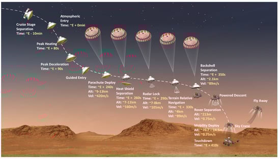
Figure 1.
Entry, descent, and landing sequence at Jezero Crater for Mars 2020 mission by NASA (Image Credit: NASA/JPL-Caltech).
The entry phase is the longest part of EDL. Furthermore, it is the most critical in terms of determining overall landing precision. The largest uncertainties within EDL are accumulated during that stage. There are three major factors that affect EDL performance during the entry phase: delivery errors at the atmospheric entry point, uncertain atmospheric conditions and wind disturbances on Mars, and errors in the estimates of aerodynamic parameters [16,17]. Accurate state and parameter estimation at the entry stage can significantly enhance the guidance and control performance of a lander, thereby giving desirable landing precision. Various aspects of Mars entry phase GNC are detailed in the aforementioned reference [1].
In contrast to other phases of EDL, there is a limited set of sensors that can be used for the entry phase navigation. In fact, all Mars missions so far have only used IMUs for entry navigation. Unless they are aided by external measurements, IMU-based navigation solutions are known to drift over time and give inadequate results for the needs of future Mars missions. Due to the entry vehicle heat-shield cover, onboard optical or radio navigation cannot be utilized during entry. In the literature, early work on improving Mars entry navigation was introduced by Pastor et al. [18]. That work proposed a set of surface or orbiting radio beacons to provide improved position solutions. IMU measurements were not included in the beacon-only filtering scheme that was presented. Furthermore, details on aerodynamic models and parameters were not provided. The authors in [19] described an IMU-based entry navigation method using a hierarchical filter architecture. Yet another IMU-based entry navigation scheme was the one introduced by Marschke et al. [20] where a multiple-model adaptive filter was utilized. The first comprehensive approach to integrated entry navigation for Mars landing was presented by Lévesque and Lafontaine [21]. The authors introduced a navigation scheme in which surface radio beacons and IMU data were fused using an unscented Kalman filter (UKF). A reasonably complete dynamic model as well as detailed observability analyses were provided for four different navigation scenarios. Robustness to any of the aforementioned error sources was not addressed in that work. Moreover, Doppler measurement, which is an important source of information, was not considered. Wu et al. [22] and Xiao et al. [23] presented an integrated navigation scheme in which unknown inputs to entry dynamics were considered. Their work illustrated the design of a robust three-stage Kalman filter to mitigate the effects of systematic errors caused by parameter uncertainties. The authors demonstrated three stages of a specific transformation that was applied in order to decouple the covariance matrices of an augmented system consisting of states and unknown inputs. The aforementioned work did not consider the estimation of the vehicle ballistic coefficient as well as the lift-to-drag ratio, which is critical for accurate control. Moreover, the unknown inputs were modeled as stochastic processes driven by white Gaussian noise. This assumption is relaxed in the present research to tackle non-Gaussian input measurement noise.
Research presented in [24] provided a mechanism to select optimized beacon locations for an integrated Mars entry navigation scheme that enhanced state estimation performance. The authors provided extensive observability analyses for various navigation scenarios. A desensitized extended Kalman filter for radio- and IMU-based entry navigation was presented by Li et al. [25]. An approach that attempted to mitigate the effects of unobservable uncertain parameters during entry was demonstrated in [26]. A multisensor approach that utilized real-time flush air data system information in addition to a single orbiting radio beacon and an IMU was detailed in [27]. An UKF was used to blend information from the three sources. This is the most recent approach in terms of adding more sensor modalities to enhance navigation performance and one that is being considered for future missions as well [28,29]. However, the authors did not consider the estimation of the vehicle ballistic coefficient nor the lift-to drag ratio, which are critical parameters for real-time entry navigation. Furthermore, the robustness of the navigation solution was not considered within its scope. Although not directly comparable to the present research, other research works that deserve mentioning involve methods that focus on a postflight analysis of EDL performance by combining data from various onboard sensors. Karlgaard et al. [30,31,32,33] produced a series of publications detailing the trajectory and atmospheric reconstruction for various Mars missions. The techniques outlined therewith were offline smoothing techniques that used data from IMU, aerodynamic, and aerothermal sensors for trajectory and atmospheric reconstruction.
1.2. Contribution
In the present research, the real-time fusion of measurements from multiple ground-based radio beacons, an IMU, and onboard environmental sensors for pressure and aeroheating is conducted to give highly accurate state and parameter estimates. The use of aerodynamic pressure and aerothermal sensor data for real-time navigation has not been realized on a Mars landing mission so far. The proposed sensor fusion is performed using a statistically robust (by statistically robust, we are referring to distributional robustness in particular) M-estimation-based iterated extended Kalman filter (MIEKF). Methods of robustifying the linear and extended Kalman filters against non-Gaussian noise have been presented in [34,35]. The present work handles non-Gaussian measurement noise in an iterated Kalman filtering context to get the added benefit of reduced linearization errors. This is a first attempt for the application considered in this paper, as far as the authors are aware. Outliers can occur in a number of realistic scenarios; in the case of sensor measurements, they can occur when sensors produce spurious data due to faults or they experience interference from external sources. The peculiar nature of noise phenomena that are influenced by outliers is that they are heavy-tailed (non-Gaussian). Hence, the conventional Gaussian noise model is inadequate to represent them. The performance of standard versions of the extended Kalman filter (EKF) and unscented Kalman filter (UKF) degrades appreciably in the face of outliers. On the contrary, the proposed method exhibits excellent performance when the Gaussian assumption on observation noise is violated. (Particle filters are good candidates for filtering in a non-Gaussian context. However, their computational expense is too high for potential onboard implementation for the application that is considered in this paper.)
Succinctly, the contribution of the present work is twofold:
- To our knowledge, this work is the first in the literature to tackle real-time multisensor Mars entry navigation in the face of non-Gaussian measurement noise. This accounts for more realistic measurement scenarios during the lander entry.
- Due to the utilization of additional sensors, the proposed scheme is, to our knowledge, the first to estimate the ballistic coefficient and reference atmospheric density independently and with high accuracy. Other related research works either estimate products of these parameters or require another projectile with a known ballistic coefficient to be launched from the entry vehicle to make the ballistic coefficient observable [21]. Other approaches involve trying to mitigate the effects of unobservable parameters on the state estimation using the considered Kalman filtering [26].
1.3. Contents of the Paper
The rest of the paper is organized as follows: Section 2 gives the details of the dynamic equations of motion and sensor observation relations. Section 3 provides a discussion on robust statistical estimation in the presence of measurement outliers. In Section 4, using the background developed in Section 3, the proposed M-estimation-based IEKF is introduced as an integrated navigation filter. Furthermore, for completeness, a brief description of alternative filtering methods is outlined in that section. In Section 5, the settings for our simulation experiments are presented. Results and discussion thereof are given in Section 6. Concluding remarks are made in Section 7. The appendices at the end of the paper provide information that supplements the main discussion.
2. Problem Formulation
2.1. Mars Entry Dynamic Equations of Motion
The geometry of motion of a Mars lander and the forces it experiences during entry are shown in Figure 2 [36].
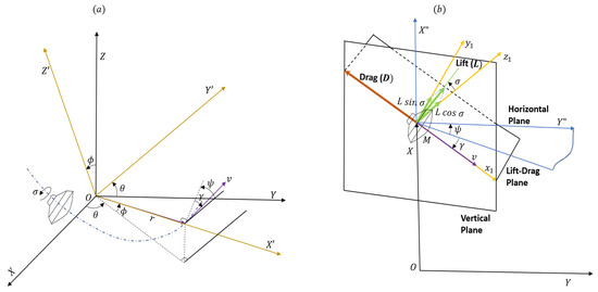
Figure 2.
(a) Geometry of motion of entry vehicle. (b) Aerodynamic forces acting on the entry vehicle.
The frame corresponds to the Mars-centered Mars-fixed (MCMF) frame, m. represents the position (vehicle-pointing) coordinate frame, p, which aligns its -axis with the position vector of the entry vehicle. Its -axis points in the direction parallel to the equatorial plane and its -axis completes a right-handed system. For the illustration showing the aerodynamic forces, we take the vertical plane to be the plane, and the lift vector L is rotated out of this plane by the bank angle . M is the position of the vehicle. ,, is an axis from the vehicle position M parallel to the vehicle-pointing axis. is a frame generated by rotating the frame by in the horizontal plane and then by in the vertical plane. The vehicle is considered as a point-mass during entry, which eliminates the need for consideration of attitude dynamics. This assumption is widely supported in the literature [16,36]. Therefore, only a three-degree-of-freedom translational model is considered in this research.
Assuming a spherical planet model, the entry equations of motion in the MCMF frame are given by
where is the range of the vehicle from the center of Mars. is the magnitude of the velocity vector, is the flight path angle measured from the local horizontal plane to the velocity vector, is the longitude, is the latitude, is the heading angle measured from east to north about the -axis where indicates a heading in the east direction, and is the commanded bank angle used as a control variable. accounts for planetary rotation. Terms involving this variable are small and can be ignored for short-range flights such as the one considered in the present work. is the gravitational constant of Mars. and are aerodynamic drag and lift accelerations, respectively, and are defined as
where is Mars’s atmospheric density, S is the reference surface area of the entry vehicle, and are the aerodynamic drag and lift coefficients, respectively. We define as the inverse of the ballistic coefficient, and the dynamic pressure is defined as . The atmospheric density (t) follows an exponential model given by
where is the reference atmospheric density of Mars, km is the reference radial position at 40 km above Mars’s surface, and km is the atmospheric scale height. The expression for can now be represented as
The control for the entry vehicle is computed using
which makes an important parameter to estimate for the purposes of accurate guidance and control. Other critical parameters to estimate are the inverse ballistic coefficient and the reference atmospheric density . Conventionally, is taken to be a constant based on empirical data assuming nominal conditions near Mars’s surface. If conditions deviate significantly from the aforementioned nominal conditions, it can drastically affect navigation performance. It is therefore important to have high-accuracy estimates of in real time during entry (Chapter 2, [37]). The augmented state and parameter vector, , is given by
We can now present the state-space representation of (1) with the aforementioned parameters augmented as constants to be estimated. In a standard state-space form, we have
by adding process noise to the expression in (7), we can describe the continuous-time entry dynamic equations of motion as
where , is the control input, and . The random vector is normally distributed and satisfies
where is the power spectral density function of , and is the Dirac delta function defined by the property (known as sifting property in signal processing).
for any real-valued function which is continuous at . The initial state vector, which we define to be , has a mean random vector given by
and its covariance is given by
we further assume that
2.2. Measurement Models
Four information sources are considered in the proposed multisensor navigation scheme: an IMU on board the entry vehicle, a set of radio beacons on Mars’s surface, an array of pressure sensors on the entry vehicle heat shield, and a set of thermocouples on the entry vehicle forebody. The measurement relations for each information source are derived below.
2.2.1. Inertial Measurement Unit (IMU)
An inertial measurement unit is used to measure the nongravitational accelerations experienced by the entry vehicle. The measurements are carried out with respect to the entry vehicle body frame. IMU observations are affected by errors such axis misalignment , scale-factor errors , biases , and random noise . The accelerometer measurement in the body frame, b, is given in terms of the true acceleration, as
where
and
the measured acceleration in the velocity coordinate frame is given by
and the velocity frame is related to the body frame by , where the definition of is given in Appendix A of this paper.
We chose the MCMF coordinate system for navigation. We therefore transformed the accelerometer measurements in the velocity frame to the MCMF frame using the following transformations.
where p represents the position coordinate frame. We finally obtained the acceleration in MCMF frame as
let . The discrete-time IMU measurements in the MCMF frame become
2.2.2. Ground-Based Radio Beacon Array
Using radio-based ranging to aid in entry navigation comes with a unique challenge. The plasma sheath around the entry body can block radio waves, thereby causing signal blackouts. However, it was indicated in [21,38] that radio beacons that work at high frequencies can overcome the signal blackout issue. We propose using three beacons that work in the UHF band placed on the surface of Mars. The Electra transceiver discussed in [39] is well suited for such an application. The placement of the beacons is such that observability is maximized according to the Fisher information criterion [24]. An illustration of the measurement setup is shown in Figure 3. The range measurement from the kth beacon to the lander is given by
where is the true range from the kth beacon to the lander, is the range bias, and is the measurement noise.
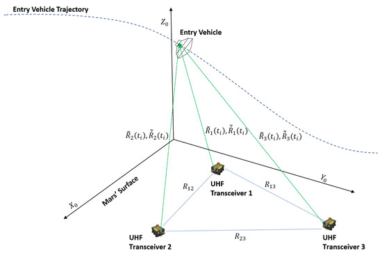
Figure 3.
UHF transceiver-based measurement scheme.
The true range is given by
where is the lander position given by
and is the known location of the kth beacon. The UHF transceivers further provide Doppler measurements. For the kth transceiver, we have
where and , . and are the lander and beacon velocity vectors respectively. For the ground-based beacons used in this research, . In vector form, we have
2.2.3. Atmospheric and Aerothermal Sensor Suite
The Mars Entry, Descent, and Landing Instrumentation (MEDLI) used in Mars Science Laboratory (MSL) and its successor MEDLI2 used in Mars 2020 has been utilized to measure atmospheric and aerothermodynamic quantities [40,41,42]. However, these measurements were only used for postflight trajectory and atmospheric reconstruction, as well as aerodynamic performance analysis purposes. The MEDLI2 sensor suite provides information on the forebody and aftbody aeroheating and pressure of the entry vehicle. A similar architecture is utilized here, but in our work, we assume a set of sensors that give us a fairly accurate characterization of the stagnation-point pressure (using forebody pressure sensors) and heating rate (using forebody thermocouples) in real time to inform onboard guidance and control actions. (Measurement accuracy can be contingent upon flight regime; for instance, pressure transducers that are accurate for hypersonic regime may not give sufficient results for supersonic flight, but these details are not considered in this research.) An illustration of the geometry of the sensors on the heat shield is given in Figure 4. We use the location of sensors proposed in [28]. (The authors in that reference considered the location of pressure sensors only; we propose a similar geometry for both pressure and heating rate sensors in the present work. On actual Mars landers, the sensor placement is done systematically using an optimization approach.) The measurement of dynamic pressure (we assumed that an aggregate measurement from all corresponding sensor arrays was used) is given by
where is the measurement noise. Upon incorporating the relation in (3), we obtain the form
the measured convective heating rate at the stagnation point is modeled by the Sutton–Graves relation [43] represented by
where k is a planet-dependent constant, which, for Mars, equals , is the vehicle nose radius, and is the heating-rate measurement noise. Substituting (3) into (29), we get
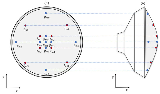
Figure 4.
(a) Layout of an array of sensors for measuring pressure (denoted by ) and heating rate (denoted by ) on the heat shield of a Mars entry vehicle. (b) An alternative view of the sensor locations geometry looking in the direction of the positive x-axis.
We now combine the measurements from all the sources mentioned so far into an aggregate measurement relation stated as
Equation (31) is finally cast as a general nonlinear observation equation of the form
where h is the surjection, . , , , and the following properties hold
where is the measurement noise covariance matrix and is the Kronecker delta function given by
moreover, we have
the key consideration made in this research is that, contrary to that of the process noise , we do not insist on the measurement noise being Gaussian. This allows us to model outlier events such as sensor faults and corrupted measurements.
3. Robust Statistical Methods in Estimation
One of the goals in statistical signal processing is estimating the parameters of signals embedded in noise [44,45]. The statistical nature of the noise is usually characterized by a Gaussian distribution. In a large number of applications, due to the central limit theorem, this assumption holds. However, when the Gaussian assumption is no longer valid, the estimation machinery that considers Gaussian noise can perform very poorly. In realistic scenarios, we are usually interested in measurement data that are contaminated by outlier of the type discussed in Section 1. Outliers are data points that are at a significant distance away from the bulk of the observed data and they render the distribution of the observations heavy-tailed [46]. Examples of well-known heavy-tailed distributions are Laplace, Cauchy, and -contaminated Gaussian distribution. Consider a linear measurement model of the form [47]
where is the observation, is the parameter to be estimated, and is the observation noise. In the Gaussian case, the observation noise density, parameterized by the mean and variance , takes the form
for Laplace and Cauchy densities, the corresponding pdfs are given by
and
respectively. The -contaminated Gaussian model is a mixture that is given by
where is the fraction of outliers in the data, is the variance of the contaminating distribution, and is the standard deviation of the mixture. The aforementioned non-Gaussian densities are shown in comparison to the Gaussian density in Figure 5. Using the -contaminated model (40), an illustration of the characteristics of outlier-contaminated Gaussian noise, , is shown in Figure 6 for varying percentages of outliers, , in the data. Distributionally robust procedures that can mitigate the increase in estimation variance in the face of heavy-tailed noise are desirable in real-world applications. One such procedure is discussed below.
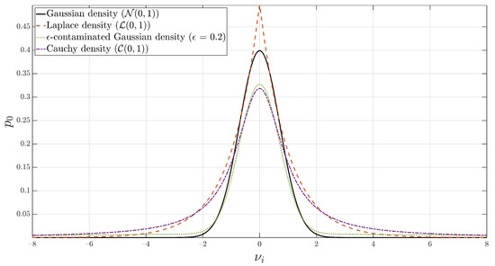
Figure 5.
Gaussian, Laplace, -contaminated Gaussian, and Cauchy densities. The latter three densities have noticeably heavier tails.
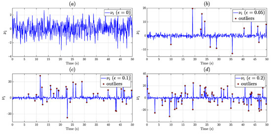
Figure 6.
Effect of additive outliers on Gaussian noise: (a) , no outlier contamination; (b) , outlier contamination; (c) , outlier contamination; (d) , outlier contamination.
Once again, considering the measurement model (36) and assuming are independent and identically distributed, the likelihood function is given by
the maximum likelihood estimator (MLE) of the parameter is the quantity which satisfies
from the monotonicity property of the logarithmic function and assuming is positive everywhere, we have
where . Equation (43) is general in that it works for all distributions satisfying the conditions imposed on . For instance, if has a normal distribution
, then we have (after ignoring constants that do not affect the optimization)
if has a Laplace distribution
then , and the MLE for becomes
taking the derivative of the negative log-likelihood function , the MLE satisfies
where . (In the statistics literature, and are used as standard symbols instead of and used in this paper. We changed the notation in order to avoid confusion with the symbols for atmospheric density and heading angle used in the equations of motion).
The function may be considered a penalty on measurement residuals (also referred to as a loss function in the literature), while the function gives a measure of the sensitivity of the estimator to outliers in the observation.
A class of estimators called M-estimators can provide outlier-robust estimates without the need for preprocessing the data [48,49]. One such estimator is the Huber M-estimator. For such an estimator, for some real r, is given by
is a hybrid of -norm penalty (corresponding to a Laplace observation noise) and -norm penalty (corresponding to a Gaussian observation noise). An illustration of the and norm penalties is shown in Figure 7.
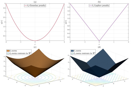
Figure 7.
(a) -norm penalty corresponding to Gaussian observation noise. (b) -norm penalty corresponding to Laplace observation noise. (c) norm given by and its contours in . (d) -norm given by and its contours in .
Differentiating (49), the sensitivity function for the Huber penalty becomes
where is a designer-chosen tuning parameter that defines the level of sensitivity of the estimator to outliers. Illustrations of and for the Huber M-estimator are shown in Figure 8. Depending on the choice of the parameter , one can design an estimator with varying degrees of response to outliers. Estimators such as the Huber M-estimator with bounded sensitivities for large residuals provide robust performance. In fact, this estimator is robust in the minimax sense [34,35], i.e., it is optimally robust against maximum performance degradation for an -deviation of data from normality assumptions.
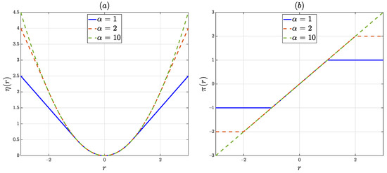
Figure 8.
(a) Loss function for the Huber M-estimator. For , the penalty for large residuals is very high, implying outliers will have a significant influence on the estimation accuracy. Alternatively, one can interpret this as the component of the Huber penalty function dominating over a wider span of residuals compared to the component of the Huber penalty. For , the slope of the curve is less steep making the contribution of outliers less influential in the estimation performance. In this case, the component of the Huber penalty has more influence on the estimation performance. gives a performance that is in between the former two. (b) Sensitivity function for the Huber M-estimator. For robustness, we desire a continuous and bounded sensitivity function [46]. Since the case of is bounded over a smaller interval of residual values, it is less sensitive to large outliers. The sensitivity increases for increasing values of .
For the case of a dynamic estimation in a Kalman filtering setting, the update stage is known to be equivalent to a static estimation problem [50]. Ruckdeschel et al. [35] proposed a Huberization of the state update derived from the Huber penalty discussed in the preceding section. In that formulation, the sensitivity function takes as an argument the Kalman filter innovations sequence. This helps mitigate large measurements (likely outliers) that enter the update equation in an unbounded manner. This seemingly ad hoc procedure has minimax optimal robustness properties. (There are some conditions attached to this result, the reader is referred to [35] for details.) We integrated this concept into an iterated extended Kalman filter to gain the benefits of the reduced linearization errors of the iterated EKF while adding robustness to non-Gaussian measurement noise.
5. Simulation Experiments
Simulation Settings
Simulation experiments were carried out in MATLAB®. Estimation results were obtained using non-Gaussian measurement noise using an -contaminated model with: ( contamination), ( contamination), and a more severe case with ( contamination). The results of each of the three scenarios are shown in Section 6. Initial conditions are taken from [21] and are shown in Table 1. Although the entry phase of EDL typically takes around 240 to 250 s, we ran our simulations for a longer time span to better visualize filter performance over a wide timeline. Time intervals in which there were outlier-influenced measurements were specified to be: 50–90 s, 170–220 s, 300–340 s, and 380–400 s (assuming outlier contamination throughout the entire entry phase is also possible in the proposed framework).

Table 1.
True and filter initial conditions for states and parameters used in simulations.
The bank angle was taken to be . The specifications of the IMU were directly taken from Table 2 in [7]. A high-end IMU option was selected. The location of radio beacons on Mars’s surface are given in Table 2.
Table 2.
UHF transceiver locations on Mars’s surface.
The filter parameters were chosen as follows:
Using the method outlined in (Chapter 9, [54]), the initial state error covariance was taken as
the process noise covariance matrix was taken to be
the measurement noise covariance was taken as (these values were chosen based on actual sensor capabilities reported in [7], where applicable).
Outliers were generated using an -contaminated model for the kth element of measurement noise vector. The model was given by (varying levels of outliers can be used in this model for each sensor depending on the prior crude knowledge of the measurement environment; here, we considered similar contamination levels for all sensors):
where is the measurement variance of each sensor (i.e., the diagonals of ). The results of our simulation studies are given below. In each case, three candidate algorithms were compared: EKF, UKF, and MIEKF.
6. Results and Discussion
Detailed plots showing the estimation performance of the proposed method and comparison with alternative approaches are provided in Figure 9, Figure 10, Figure 11, Figure 12, Figure 13, Figure 14, Figure 15, Figure 16, Figure 17 and Figure 18. Figure 9 shows the estimation performance of the various filters in the presence of a relatively mild outlier level of .
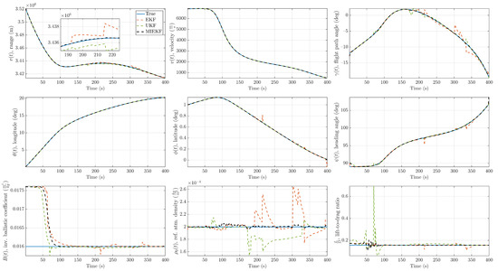
Figure 9.
State estimation performance comparison for 5% outlier contamination ().
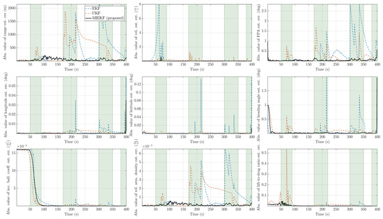
Figure 10.
Absolute value of estimation errors with for the three candidate filters (the time intervals shaded in light green are intervals in which outliers are present).
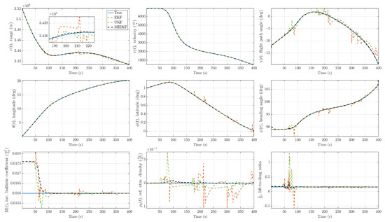
Figure 11.
State estimation performance comparison for 20% outlier contamination ().
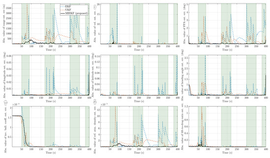
Figure 12.
Absolute value of estimation errors with for the three candidate filters (the time intervals shaded in light green are intervals in which outliers are present).
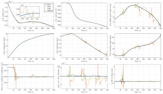
Figure 13.
State estimation performance comparison for 40% outlier contamination ().
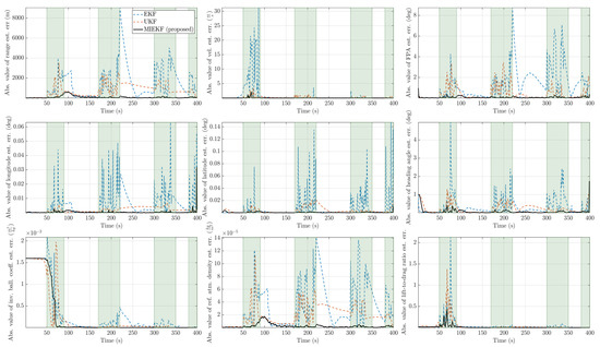
Figure 14.
Absolute value of estimation errors with for the three candidate filters (the time intervals shaded in light green are intervals in which outliers are present).
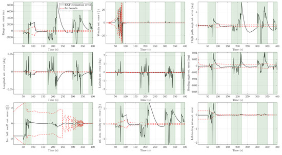
Figure 15.
EKF estimation errors with bounds for (the time intervals shaded in light green are intervals in which outliers are present).
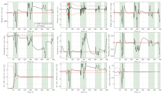
Figure 16.
UKF estimation errors with bounds for (the time intervals shaded in light green are intervals in which outliers are present).
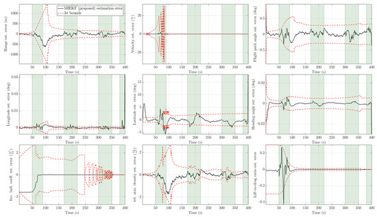
Figure 17.
MIEKF estimation errors with bounds for (the time intervals shaded in light green are intervals in which outliers are present).
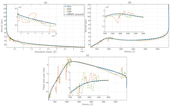
Figure 18.
For : (a) Atmospheric density variation with altitude. (b) Velocity variation with altitude. (c) Relationship between velocity and flight path angle. It is noteworthy that MIEKF-based estimates are not affected by outliers and match the true relationships quite closely, while alternative approaches exhibit noticeable errors in estimation.
The state estimates for the proposed method showed good adherence to the true values while alternative methods deviated from the true values during the time intervals where outlier influences occurred. The absolute values of the estimation errors are depicted in Figure 10. In this figure, one can see the clear performance benefits of the MIEKF-based navigation (shown in a solid black line) in outlier-influenced time intervals (shown in light green). The MIEKF maintained a low estimation error throughout the simulation. We see a similar pattern for the case of outlier levels in Figure 11 and Figure 12. The estimation errors for all filters were correspondingly higher with a higher level of outliers. However, the MIEKF performance degraded only marginally, while the performance degradation in other filters was noticeable. Overall, the MIEKF still maintained the lowest estimation error among all the filters considered in this research.
An outlier level of is considered a high level of contamination. The trend we observed in the previous two cases persisted in that case as well. This is shown in Figure 13 and Figure 14. The MIEKF provided the lowest estimation errors among the alternatives. The filter consistency plots in Figure 15, Figure 16 and Figure 17 show that only the MIEKF-based estimates give a good agreement with the theoretically predicted performance. The estimates based on alternative approaches tend to show divergence within outlier-influenced regions and in some cases, they show hang-off errors.
Plots for the relationship between altitude and atmospheric density, altitude and velocity, as well as flight path angle and velocity are provided in Figure 18. This gives yet another perspective on the enhanced performance of MIEKF. In passing, we note that if the conventional Gaussian assumption for measurement noise (i.e., no outliers) is assumed throughout the simulation duration, the UKF performs the best on a majority of the state estimates.
As a final demonstration of the effectiveness of the proposed method, we provide numerical RMSE values to show what level of performance we can expect from the proposed multisensor navigation scheme. This is shown in Table 3. MIEKF consistently performs better than the alternative approaches. For most states, the margin of improvement is substantial.
Table 3.
Filter performance comparison based on RMSE values.
7. Conclusions
A statistically robust sensor fusion framework for autonomous entry phase navigation for Mars landing was presented. The method added positioning accuracy and parameter observability by virtue of the multisensor approach and added distributional robustness to non-Gaussian noise due to the M-estimation-based filter employed to fuse the data from the sensors. The method had a similar computational complexity to existing tried and proven filtering methods. The present design can account for sensor faults or external sources of spurious data that lead to outliers. In space, these events can be frequent. Future Mars pinpoint landing missions require that landers touch down within an error ellipse of at most 50 m around the chosen landing site. The main challenge in meeting this requirement has been the limitation of inertial-only navigation during entry. By employing a multimodal approach in a robust sensor fusion architecture, the research in this paper, after additional practical considerations, has the potential to enable a highly accurate entry phase navigation. Combining the advantages of the iterated extended Kalman filter (IEKF) with the robustness properties of the M-estimation, the proposed M-estimation-based IEKF (MIEKF) performed better than alternative approaches. We substantiated our claim with experiments showing the estimation error performance for each candidate method. There are several additional problems that require attention in future work. With eventual onboard implementation in mind, using more stable versions of the covariance propagation using factorization methods is required to avoid potential numerical problems. Accounting for uncertainties in radio beacon location is an important consideration that warrants attention. The assumption of a fairly accurate knowledge of entry conditions is a serious limitation of the present work. The use of X-ray pulsar-based navigation during the approach phase of Mars Entry, Descent, and Landing (EDL) to improve knowledge of entry conditions is a promising technique. A more rigorous derivation of a different version of the MIEKF directly from a maximum likelihood formulation is being developed by the authors for future work. This will avoid some ad hoc assumptions presented in this paper that may reduce estimation efficiency. Applying the distributionally robust sensor fusion method discussed in this work to other phases of EDL, where more navigation sensors such as cameras and radar are available, is yet another interesting avenue to consider.
Author Contributions
Conceptualization, N.S.Z.; methodology, N.S.Z.; software, N.S.Z.; validation, N.S.Z.; formal analysis, N.S.Z.; investigation, N.S.Z.; resources, N.S.Z.; data curation, N.S.Z.; writing—original draft preparation, N.S.Z.; writing—review and editing, N.S.Z.; visualization, N.S.Z.; supervision, H.B. All authors have read and agreed to the published version of the manuscript.
Funding
This research received no external funding.
Data Availability Statement
Data sharing not applicable.
Acknowledgments
The authors would like to thank the anonymous reviewers for the valuable feedback they provided.
Conflicts of Interest
The authors declare no conflict of interest.
Appendix A. Coordinate Frame Definitions and Transformations
- (1)
- Mars-centered inertial (MCI) frame ():It is centered on the planet and its z-axis aligned with Mars’s rotation axis, x-axis pointing towards the vernal equinox, and the y-axis completes a right-handed system.
- (2)
- Mars-centered Mars-fixed (MCMF) frame (m):It is fixed to the planet and rotates with it. It shares the same rotation axis with the planet and hence the MCI frame. A rotation of about the MCI frame’s z-axis gives the MCMF frame. The transformation between the two frames is
- (3)
- Vehicle-pointing/position coordinate system (p):It originates at the planet’s center with its x-axis pointing in the direction of the vehicle’s position vector. Its y-axis points parallel to the equatorial plane and its z-axis completes a right-handed system. The transformation from the position coordinate frame to the MCMF frame can be done using the following matrix
- (4)
- Body frame (b):Its origin is the vehicle center of mass. The axes for this frame are configured to align with each axis of symmetry of the entry vehicle. IMU measurements are defined in this coordinate frame.
- (5)
- Velocity frame (v):Its origin is centered on the lander vehicle with its x-axis aligned in the direction of the flight path, its z-axis lies on a local vertical plane orthogonal to the x-axis, and the y-axis completes a right-handed system. The transformation from the velocity frame to the vehicle-pointing frame is given byand the transformation from the velocity frame to the body frame is given bywhere is the bank angle and is the angle of attack of the entry vehicle.
Appendix B. Derivation of the Standard Iterated Extended Kalman Filter (IEKF) via an Optimization Approach
Consider the state-space formulation (51) and (52). Using a Bayesian approach, the posterior density is related, up to a constant, to the likelihood and the prior pdf by
the maximum a posteriori (MAP) estimate is given by
by taking the negative logarithm of the expression in (A5) and setting
we have
let
then the MAP estimate becomes
Equation (A10) is a nonlinear least squares problem, which in this case, we solve using the Gauss–Newton method as it does not require the computation of second-order derivatives. The gradient of is given by
where .
An approximation of the Hessian is given by
The Gauss–Newton iteration is carried out using (the simplest case of a fixed step size is assumed) [55,56]
with
where . Substituting the quantities computed so far into the Gauss–Newton iteration (A13) yields
rearranging (A15) and using the property
which follows from the matrix inversion lemma, we have the final form of the IEKF state update iteration as
References
- Li, S.; Jiang, X. Review and Prospect of Guidance and Control for Mars Atmospheric Entry. Prog. Aerosp. Sci. 2014, 69, 40–57. [Google Scholar] [CrossRef]
- NASA Technology Taxonomy. 2020. Available online: https://www.nasa.gov/offices/oct/taxonomy/index.html (accessed on 7 December 2022).
- Starek, J.A.; Açikmese, B.; Nesnas, I.A.D.; Pavone, M. Spacecraft Autonomy Challenges for Next-Generation Space Missions. In Advances in Control System Technology for Aerospace Applications; Feron, E., Ed.; Lecture Notes in Control and Information Sciences 460; Springer: Berlin/Heidelberg, Germany, 2016; pp. 1–41. [Google Scholar]
- Yu, Z.; Cui, P.; Crassidis, J.L. Design and Optimization of Navigation and Guidance Techniques for Mars Pinpoint Landing: Review and Prospect. Prog. Aerosp. Sci. 2017, 94, 82–94. [Google Scholar] [CrossRef]
- Braun, R.D.; Manning, R.M. Mars Exploration Entry, Descent, and Landing Challenges. J. Spacecr. Rockets 2007, 44, 310–323. [Google Scholar] [CrossRef]
- Lugo, R.A.; Cianciolo, A.D.; Williams, R.A.; Dutta, S.; Powell, R.W.; Chen, P.T. Integrated Precision Landing Performance and Technology Assessments of a Human-Scale Mars Lander Using a Generalized Simulation Framework. In Proceedings of the AIAA SCITECH 2022 Forum, San Diego, CA, USA, 3–7 January 2022; pp. 1–15. [Google Scholar]
- Cianciolo, A.D.; Striepe, S.; Carson, J.; Sostaric, R.; Woffinden, D.; Karlgaard, C.; Lugo, R.; Powell, R.; Tynis, J. Defining Navigation Requirements for Future Precision Lander Missions. In Proceedings of the AIAA Scitech Forum, San Diego, CA, USA, 7–11 January 2019; pp. 1–18. [Google Scholar]
- Carson, J.; Munk, M.; Sostaric, R.; Johnson, A.; Amzajerdian, F.; Blair, J.B.; Matthies, L. Precise and Safe Landing Navigation Technologies for Solar System Exploration. Bull. AAS 2021, 53, 413. [Google Scholar] [CrossRef]
- Williams, J.W.; Woffinden, D.C.; Putnam, Z.R. Mars Entry Guidance and Navigation Analysis Using Linear Covariance Techniques for the Safe and Precise Landing—Integrated Capabilities Evolution (Splice) Project. In Proceedings of the AIAA Scitech Forum, Orlando, FL, USA, 6–10 January 2020; pp. 1–19. [Google Scholar]
- Woffinden, D.C.; Robinson, S.B.; Williams, J.W.; Putnam, Z.R. Linear Covariance Analysis Techniques to Generate Navigation and Sensor Requirements for the Safe and Precise Landing—Integrated Capabilities Evolution (SPLICE) Project. In Proceedings of the AIAA Scitech Forum, San Diego, CA, USA, 7–11 January 2019. [Google Scholar]
- Prakash, R.; Burkhart, P.D.; Chen, A.; Comeaux, K.A.; Guernsey, C.S.; Kipp, D.M.; Lorenzoni, L.V.; Mendeck, G.F.; Powell, R.W.; Rivellini, T.P.; et al. Mars Science Laboratory Entry, Descent, and Landing System Overview. In Proceedings of the 2008 IEEE Aerospace Conference, Big Sky, MT, USA, 1–8 March 2008; pp. 1–18. [Google Scholar]
- Nelessen, A.; Sackier, C.; Clark, I.; Brugarolas, P.; Villar, G.; Chen, A.; Stehura, A.; Otero, R.; Stilley, E.; Way, D.; et al. Mars 2020 Entry, Descent, and Landing System Overview. In Proceedings of the 2019 IEEE Aerospace Conference, Big Sky, MT, USA, 2–9 March 2019; pp. 1–20. [Google Scholar]
- Blackmore, L.; Açikmeşe, B.; Scharf, D.P. Minimum-Landing-Error Powered-Descent Guidance for Mars Landing Using Convex Optimization. J. Guid. Control Dyn. 2010, 33, 1161–1171. [Google Scholar] [CrossRef]
- Açıkmese, B.; Casoliva, J.; Carson, J.M., III. G-FOLD: A Real-Time Implementable Fuel Optimal Large Divert Guidance Algorithm for Planetary Pinpoint Landing. In Proceedings of the Concepts Approaches Mars Exploration, Houston, TX, USA, 12–14 June 2012. [Google Scholar]
- Bishop, R.H.; Crain, T.P.; Hanak, C.; DeMars, K.; Carson, J.M.; Trawny, N.; Christiank, J. An Inertial Dual-State State Estimator for Precision Planetary Landing with Hazard Detection and Avoidance. In Proceedings of the AIAA Guidance, Navigation, and Control Conference, San Diego, CA, USA, 4–8 January 2016; pp. 1–21. [Google Scholar]
- Lévesque, J.F. Advanced Navigation and Guidance for High-Precision Planetary Landing on Mars. Ph.D. Thesis, University of Sherbrooke, Quebec, QC, Canada, 2006. [Google Scholar]
- Wolf, A.A.; Graves, C.; Powell, R.; Johnson, W. Systems for Pinpoint Landing at Mars. Adv. Astronaut. Sci. 2005, 119, 2677–2696. [Google Scholar]
- Pastor, P.R.; Gay, R.S.; Striepe, S.A.; Bishop, R.H. Mars Entry Navigation from EKF Processing of Beacon Data. In Proceedings of the Astrodynamics Specialist Conference, Denver, CO, USA, 14–17 August 2000; pp. 518–528. [Google Scholar]
- Bishop, R.H.; Dubios-Matra, O.; Ely, T. Robust Entry Navigation using Hierarchical Filter Architectures Regulated with Gating Networks. In Proceedings of the 16th International Symposium on Space Flight Dynamics, Pasadena, CA, USA, 3–6 December 2001. [Google Scholar]
- Marschke, J.M.; Crassidis, J.L.; Lam, Q.M. Multiple Model Adaptive Estimation for Inertial Navigation during Mars Entry. In Proceedings of the AIAA/AAS Astrodynamics Specialist Conference and Exhibit, Honolulu, HI, USA, 18–21 August 2008. [Google Scholar]
- Lévesque, J.F.; De Lafontaine, J. Innovative Navigation Schemes for State and Parameter Estimation during Mars Entry. J. Guid. Control Dyn. 2007, 30, 169–184. [Google Scholar] [CrossRef]
- Wu, Y.; Fu, H.; Xiao, Q.; Zhang, Y. Extension of Robust Three-Stage Kalman Filter for State Estimation during Mars Entry. IET Radar Sonar Navig. 2014, 8, 895–906. [Google Scholar] [CrossRef]
- Xiao, M.; Zhang, Y.; Wang, Z.; Fu, H. Augmented Robust Three-Stage Extended Kalman Filter for Mars Entry-Phase Autonomous Navigation. Int. J. Syst. Sci. 2018, 49, 27–42. [Google Scholar] [CrossRef]
- Yu, Z.; Cui, P.; Zhu, S. Observability-Based Beacon Configuration Optimization for Mars Entry Navigation. J. Guid. Control Dyn. 2015, 38, 643–650. [Google Scholar] [CrossRef]
- Li, S.; Jiang, X.; Liu, Y. High-Precision Mars Entry Integrated Navigation under Large Uncertainties. J. Navig. 2014, 67, 327–342. [Google Scholar] [CrossRef]
- Lou, T.; Fu, H.; Zhang, Y.; Wang, Z. Consider Unobservable Uncertain Parameters Using Radio Beacon Navigation during Mars Entry. Adv. Space Res. 2015, 55, 1038–1050. [Google Scholar] [CrossRef]
- Jiang, X.; Li, S.; Huang, X. Radio/FADS/IMU Integrated Navigation for Mars Entry. Adv. Space Res. 2018, 61, 1342–1358. [Google Scholar] [CrossRef]
- Lugo, R.A.; Karlgaard, C.D.; Powell, R.W.; Cianciolo, A.D. Integrated Flush Air Data Sensing System Modeling for Planetary Entry Guidance with Direct Force Control. In Proceedings of the AIAA Scitech Forum, San Diego, CA, USA, 7–11 January 2019; pp. 1–14. [Google Scholar]
- Karlgaard, C.D.; Stoffel, T.D.; White, T.R.; West, T.K. Data Fusion of In-Flight Aerothermodynamic Heating Measurements Using Kalman Filtering. In Proceedings of the AIAA Aviation 2022 Forum, Chicago, IL, USA, 27 June–1 July 2022; pp. 1–13. [Google Scholar]
- Karlgaard, C.D.; Tynis, J.A. Mars Phoenix EDL Trajectory and Atmosphere Reconstruction Using NewSTEP; NASA/TM-2019-220282; NASA: Washington, DC, USA, 2019. [Google Scholar]
- Karlgaard, C.D.; Korzun, A.M.; Schoenenberger, M.; Bonfiglio, E.P.; Kass, D.M.; Grover, M.R. Mars InSight Entry, Descent, and Landing Trajectory and Atmosphere Reconstruction. J. Spacecr. Rockets 2021, 58, 865–878. [Google Scholar] [CrossRef]
- Karlgaard, C.D.; Kutty, P.; Schoenenberger, M.; Munk, M.M.; Little, A.; Kuhl, C.A.; Shidner, J. Mars Science Laboratory Entry Atmospheric Data System Trajectory and Atmosphere Reconstruction. J. Spacecr. Rockets 2014, 51, 1029–1047. [Google Scholar] [CrossRef]
- Karlgaard, C.D.; Schoenenberger, M.; Dutta, S.; Way, D.W. Mars Entry, Descent, and Landing Instrumentation 2 Trajectory, Aerodynamics, and Atmosphere Reconstruction. In Proceedings of the AIAA Scitech Forum, San Diego, CA, USA, 3–7 January 2022. [Google Scholar]
- Cipra, T.; Romera, R. Robust Kalman Filter and Its Application in Time Series Analysis. Kybernetika 1991, 27, 481–494. [Google Scholar]
- Ruckdeschel, P.; Spangl, B.; Pupashenko, D. Robust Kalman tracking and smoothing with propagating and non-propagating outliers. Stat. Pap. 2014, 55, 93–123. [Google Scholar] [CrossRef]
- Vinh, N.X.; Busemann, A.; Culp, R.D. Hypersonic and Planetary Entry Flight Mechanics; The University of Michigan Press: Ann Arbor, MI, USA, 1980. [Google Scholar]
- Regan, F.J.; Anandakrishnan, S.M. Dynamics of Atmospheric Re-Entry; AIAA Education Series; AIAA: Washington DC, USA, 1993. [Google Scholar]
- Morabito, D.D. The Spacecraft Communications Blackout Problem Encountered during Passage or Entry of Planetary Atmospheres; IPN Progress Report 42-150; NASA: Washington, DC, USA, 2002; pp. 42–150. [Google Scholar]
- Lightsey, E.G.; Mogensen, A.E.; Burkhart, P.D.; Ely, T.A.; Duncan, C. Real-Time Navigation for Mars Missions Using the Mars Network. J. Spacecr. Rockets 2008, 45, 519–533. [Google Scholar] [CrossRef]
- Gazarik, M.J.; Wright, M.J.; Little, A.; Cheatwood, F.M.; Herath, J.A.; Munk, M.M.; Novak, F.J.; Martinez, E.R. Overview of the MEDLI Project. In Proceedings of the 2008 IEEE Aerospace Conference, Big Sky, MT, USA, 1–8 March 2008; pp. 1–12. [Google Scholar]
- Hwang, H.H.; Bose, D.; White, T.R.; Wright, H.S.; Schoenenberger, M.; Kuhl, C.A.; Trombetta, D.; Santos, J.A.; Oishi, T.; Karlgaard, C.D.; et al. Mars 2020 Entry, Descent and Landing Instrumentation 2 (Medli2). In Proceedings of the 46th AIAA Thermophysics Conference, Washington DC, USA, 13–17 June 2016; pp. 1–13. [Google Scholar]
- White, T.R.; Mahzari, M.; Miller, R.A.; Tang, C.Y.; Monk, J.; Santos, J.A.B.; Karlgaard, C.D.; Alpert, H.S.; Wright, H.S.; Kuhl, C. Mars Entry Instrumentation Flight Data and Mars 2020 Entry Environments. In Proceedings of the AIAA SCITECH 2022 Forum, San Diego, CA, USA, 3–7 January 2022; pp. 1–17. [Google Scholar]
- Benito, J.; Mease, K.D. Reachable and Controllable Sets for Planetary Entry and Landing. J. Guid. Control Dyn. 2010, 33, 641–654. [Google Scholar] [CrossRef]
- Kay, S.M. Fundamentals of Statistical Signal Processing: Estimation Theory; Prentice Hall: Hoboken, NJ, USA, 1997. [Google Scholar]
- Van Trees, H.L.; Bell, K.L.; Tian, Z. Detection Estimation and Modulation Theory, Part I: Detection, Estimation, and Filtering Theory; Wiley: Hoboken, NJ, USA, 2013. [Google Scholar]
- Hampel, F.R.; Ronchetti, E.M.; Rousseeuw, P.J.; Stahel, W.A. Robust Statistics: The Approach Based on Influence Functions; Wiley: Hoboken, NJ, USA, 2005. [Google Scholar]
- Maronna, R.A.; Martin, R.D.; Yohai, V.J.; Salibiàn-Barrera, M. Robust Statistics: Theory and Methods (with R); Wiley: Hoboken, NJ, USA, 2019. [Google Scholar]
- Zoubir, A.M.; Koivunen, V.; Ollila, E.; Muma, M. Robust Statistics for Signal Processing; Cambridge University Press: Cambridge, UK, 2018. [Google Scholar]
- Huber, P.; Ronchetti, E.M. Robust Statistics; Wiley: Hoboken, NJ, USA, 2009. [Google Scholar]
- Bell, B.M.; Cathey, F.W. The Iterated Kalman Filter Update as a Gauss—Newton Method. IEEE Trans. Autom. Contr. 1993, 38, 294–297. [Google Scholar] [CrossRef]
- Maybeck, P.S. Stochastic Models, Estimation and Control; Academic Press: New York, NY, USA, 1982; Volume 2. [Google Scholar]
- Simon, D. Optimal State Estimation: Kalman, H Infinity, and Nonlinear Approaches; Wiley-Interscience: Hoboken, NJ, USA, 2006. [Google Scholar]
- Julier, S.J.; Uhlmann, J.K. Unscented Filtering and Nonlinear Estimation. Proc. IEEE 2004, 92, 401–422. [Google Scholar] [CrossRef]
- Zarchan, P.; Musoff, H. Fundamentals of Kalman Filtering: A Practical Approach, 4th ed.; American Inst of Aeronautics & Astronautics: Reston, VA, USA, 2015. [Google Scholar]
- Havlík, J.; Straka, O. Performance Evaluation of Iterated Extended Kalman Filter with Variable Step-Length. J. Phys. Conf. Ser. 2015, 659, 12022. [Google Scholar] [CrossRef]
- Skoglund, M.A.; Hendeby, G.; Axehill, D. Extended Kalman Filter Modifications Based on an Optimization View Point. In Proceedings of the International Conference on Information Fusion, Washington, DC, USA, 6–9 July 2015. [Google Scholar]


Disclaimer/Publisher’s Note: The statements, opinions and data contained in all publications are solely those of the individual author(s) and contributor(s) and not of MDPI and/or the editor(s). MDPI and/or the editor(s) disclaim responsibility for any injury to people or property resulting from any ideas, methods, instructions or products referred to in the content. |
© 2023 by the authors. Licensee MDPI, Basel, Switzerland. This article is an open access article distributed under the terms and conditions of the Creative Commons Attribution (CC BY) license (https://creativecommons.org/licenses/by/4.0/).