Article

Detection and Attribution of Alpine Inland Lake Changes by Using Random Forest Algorithm

1
Department of Earth and Environmental Sciences, Xi’an Jiaotong University, Xi’an 710049, China
2
Institute of Global Environmental Change, Xi’an Jiaotong University, Xi’an 710049, China
3
Department of Geography, University of California, Los Angeles, CA 90095, USA
*
Author to whom correspondence should be addressed.
Remote Sens. 2023, 15(4), 1144; https://doi.org/10.3390/rs15041144
Submission received: 21 November 2022 / Revised: 13 January 2023 / Accepted: 30 January 2023 / Published: 20 February 2023
(This article belongs to the Special Issue Remote Sensing of Land Water Bodies)

Abstract

:
The alpine inland lake dynamics have been good indicators of changes in terrestrial hydrological cycles under global climate change. However, the relationship between alpine inland lake and climatic factors remained largely uncertain. This study examines the spatial-temporal change of the fluctuation of the lake by using dense time series Landsat TM/ETM/OLI images to delineate water boundary information based on the Random Forest algorithm and using ICESat (Ice, Cloud and land Elevation Satellite) dataset to monitor changes in variations of water level. Variations of Qinghai Lake (QHL) were analyzed from 1987 to 2020 and the mechanism of these changes was discussed with meteorological data. The results indicated that the QHL fluctuated strongly showing a pattern of shrinkage–expansion over the last three decades. The lake storage significantly decreased by −2.58 × 10⁸ m3·yr−1 (R2 = 0.86, p < 0.01) from 1989 to 2004 and sharply increased (6.92 × 10⁸ m3·yr−1, R2 = 0.92, p < 0.01) after 2004. The relationship between the lake and climate over the last 30 years implies that the decreasing evaporation and increasing precipitation were the major factors affecting the fluctuation of lake storage. Meanwhile, the temporal heterogeneity of the driving mechanism of climate change led to the phased characteristics of lake storage change. In detail, obvious warming led to the shrinkage of the QHL before 2004 through increasing evaporation, while humidifying and accelerating wind stilling dominated the expansion of the QHL after 2004 by increasing precipitation and decreasing evaporation. This paper indicated that the frameworks of multi-source remote sensing and accurate detection of water bodies were required to protect the high-altitude lakes from further climate changes based on the findings of this paper of the QHL recently. The framework presented herein can provide accurate detection and monitoring of water bodies in different locations in the Qinghai-Tibet Plateau, and provide a necessary basis for future political activities and decisions in terms of sustainable water resource management.

1. Introduction

Alpine inland lake changes indicate the dynamic of the terrestrial hydrological cycle under climate change in the past decades [1,2,3,4,5]. Several studies have presented the ecological, morphological, and coverage changes of the alpine inland lake [6,7,8,9,10]. Serious inland lake water loss shows a considerable hazard to the environment such as land degradation, soil salinization, and biodiversity loss [2,11,12,13,14]. Therefore, the fluctuations (e.g., variations of area, water level, water storage) of alpine lakes are sensitive indicators of climate variability due to the minimal disturbances by human activities. Thus, assessment of the fluctuation, as a measure of the region's ecological health, is critical to the local water resource management and the hydrological process prediction according to climate change.
Satellite datasets are particularly useful for terrestrial monitoring in remote and inaccessible alpine regions, such as alpine inland lake changes. In recent decades, multi-source remote sensing images can provide land observations of high temporal and spatial resolutions, which has advantages in detecting the dynamics of alpine lakes in the Qinghai-Tibet Plateau (QTP) [9,11,15,16,17,18]. The common passive optical sensors to monitor the water feature delineation are the Landsat series Multispectral Scanner (MSS), Thematic Mapper (TM), and Enhanced Thematic Mapper Plus (ETM+), Advanced Very High-Resolution Radiometer (AVHRR), Satellite Pour l’Observation de la Terre (SPOT), and Moderate Resolution Imaging Spectroradiometer (MODIS). Thematic classification methods [19,20,21,22], single-band threshold methods [21,23], and spectral water index methods [21,24,25] were developed to map water features with visible/infrared imagery. All existing methods are using thresholds or making decision rules for different water features, which are the major sources of uncertainty in lake changes.
Machine learning approaches have been essential tools to handle multi-dimensional and highly auto-correlated data and to classify very complex features without overfitting [26]. Such cases can be encountered in satellite-based studies where the heterogeneous datasets are often complex with high-dimensional features and nonlinear with many missing values between the measured variables. For example, Random Forest (RF), one of the newly popular machine learning algorithms, is good at handling high-dimensional features that are insensitive to the outlier (noise). Therefore, among the non-parametric methods, RF is a commonly used method in image classification, which can be a better lake area identification method. In addition, ICESat (Ice, Cloud and land Elevation Satellite) acquires massive amounts of LiDAR data, providing detailed and precise measurements of heights of ice, land surface, water and clouds. The dataset has been extensively implemented to monitor changes in variations in water level [9,27,28]. Combined with the accurate measurements of the lake area and water level, lake storage anomaly could be estimated to support the more comprehensive investigations on lake dynamics and hydrological cycle process in alpine regions.
Qinghai Lake (QHL) is the largest closed-basin lake in China. It is on the northeastern margin of the QTP, which is situated at the transition from the arid to the semi-arid climate zones. The research of QHL becomes a hot topic for the Asian climate and environmental change. In the last century, the QHL has experienced severe changes in water bodies. The lake area had shrunk dramatically and obviously fallen to the water level. These changes in the water body led to a series of environmental problems such as the loss of grazing grassland, deterioration of water quality and the expansion of desertification around the beach area. Therefore, in early studies, numerous scholars strongly believed that the QHL would not dry up in a short time, but the water level would continue to decline [29,30]. However, after 2004, the water boundary of the QHL rebounded year by year. Indeed, the dominant driving factors behind lake-level changes of the QHL are still under investigation, especially the changing precipitation and evaporation patterns before and after the 2000s. Numerous previous studies have explored the change mechanisms of the QHL [31,32,33,34,35,36,37,38,39]. However, the driving mechanism of lake area variations still remained unclear. Most studies have suggested that precipitation has dominated the variations of the QHL by changing the water balance [34,35], whereas other studies concluded that evaporation had strong influences on lake change [31], and some research found that temperature indicated indirect effects on the hydrological process [37,39]. In addition, phased characteristics of climate change determined the temporal heterogeneity of the driving mechanism of lake change [12]. Therefore, a comprehensive quantitative analysis of the relative weighting of the impacts of climatic factors would make the attribution of a hydrological process of the QHL more reliable, which would be a guide for the future ecology of alpine lakes.
Global climate change has greatly affected the terrestrial hydrological cycle in recent decades [12]. QTP, the third pole of the world, is one of the most vulnerable regions to climate variations because of its complex responses and significantly associated impacts on the region [40,41,42,43]. Accurate estimation of the seasonal and inter-annual water body changes in the alpine inland lake is not only important to enhance our understanding of their responses to climate change, but also crucial to hydrological process modeling for efficient use of water resources [2,44,45,46]. Though lots of previous research has determined various driving forces by correlation analysis, their contributions by quantitative methods have rarely been seen [9,12,47,48,49,50]. The main driving forces behind the lake changes of QHL are unclear, especially the changing precipitation and evaporation patterns in the accelerating lake variations in different periods. Hence, this study aimed to explore the spatiotemporal dynamics of lake change, investigate the driving factors of the lake fluctuation, quantify each of their contributions by using machine learning techniques and further reveal the underlying mechanism of driving factors.

2. Data and Methods

2.1. Study Area

QHL, the largest inland salt-water lake in China, has a very important ecological position for natural shelter and climate regulation of Qinghai-Tibet Plateau. The QHL area is about 4300 km2 with a catchment of approximately 29,600 km2 (from 36°15′N to 38°20′N and 97°50′E to 101°20′E) (Figure 1). The cold and dry winter in the catchment is controlled by the Siberian High and the Mongolian High, while warm and wet summer is dominated by the East Asian monsoon. The annual total precipitation is about 350 mm from the historical records. The QHL is an essential water and wetland conservation area of western China, which is identified by the Ramsar Convention List of Wetlands of International Importance. In recent years, land degradation, soil salinization, and biodiversity loss took place and the surrounding wetlands were decreasing, which was caused by global climate change and unreasonable resource development and management. These phenomena indicate ecological deterioration trend of the lake basin gradually.

2.2. Data Used

2.2.1. Optical Images for Measuring Lake Area Variations

The feasibility of mapping the spatial-temporal change of the QHL was accessed by using the multi-temporal Landsat images. Notably, 34 scenes of the Landsat TM/ETM/OLI images over the study area (25 scenes of Landsat 5 TM for the years 1987 to 2011, 1 scene of Landsat 7 ETM+ for the years 2012, 8 scenes of Landsat 8 OLI for 2013 to 2020) were used to retrieve the lake surface extent from 1987 to 2020. Those satellite images of October of each year were chosen to reduce the influence of lake seasonality. The selected images are cloudless or slightly cloudy in order to extract the boundary of the QHL.

2.2.2. Satellite Altimetry Data Measuring Water-Level Variations

The ICESat/GLAS (Geoscience Laser Altimeter System) and ICESat-2/ATLAS (Advanced Topographic Laser Altimeter System) datasets were used to measure water-level variations of the QHL. ICESat, operated from 2003 to 2009, was the world’s first spaceborne laser altimetry satellite, which could collect detailed and precise measurements of heights of ice, land surface, water, and clouds. ICESat-2, launched in 2018, was a subsequent satellite to ICESat, continuing the measurement mission [51]. The datasets have been extensively implemented to monitor changes in polar ice sheets and variations in lake water levels [27].

2.2.3. Observed Water Level and Lake Area Data

Observed water levels in the Xiashe hydrological station were used to verify the validity of ICESat datasets. The Xiashe hydrological station, built in 1959, is the only station to monitor the water level on the QTP for decades, mainly monitoring the water level, precipitation and evaporation of Qinghai Lake. The time series dataset of the lake area on Qinghai-Tibet Plateau, provided by National Tibetan Plateau Data Center (TPDC), was used to assess the lake-water extraction based on the RF model.

2.2.4. Climate Datasets

The CMFD (China Meteorological Forcing Dataset) from 1987 to 2018 was used in this study. The dataset contains a series of monthly land surface parameters in China in 0.1-degree resolution. Precipitation, near-surface air temperature, surface downward shortwave radiation, near-surface wind speed, and near-surface specific humidity were selected to indicate climate variations and identify the correlation with lake change during the past three decades over the QHL.

2.3. Data Process

2.3.1. Calculation of Lake Storage Anomaly

Lake storage is a key indicator of lake change. In this study, lake area measured by Landsat images and water level measured by ICESat datasets were used to calculate the change in lake storage relative to the previous year. The change in lake storage is determined by Equation (1):
V = 1 3 H 2 H 1 × A 1 + A 2 + A 1 × A 2
where V [m3] represents the lake storage change; A 1 and A 2 are the lake areas [m2] in previous and current year; H 1 and H 2 are the water levels [m] in previous and current year. Therefore, the lake storage anomaly could be calculated by accumulating the storage.

2.3.2. Trend Analysis

During a given period (e.g., 1987–2004 or 2004–2010), a least-squares linear regression was used to find the variation between lake area and climate variables (temperature, precipitation, evaporation), as follows:
y = a + b t
where y represents lake area or climate variable, t is the year, a and b are fitted variables ( a is the intercept and b is the slope).
Moreover, a piecewise regression model was used to find the magnitude of changes among the observations and when the changes took place since it was effective to detect the turning points in the time-series data with noise:
y = β 0 + β 1 t + ε ,                                             t α β 0 + β 1 t + β 2 t α + ε ,                       t > α
where t is the year; α is the estimated turning point of the time series; β 0 , β 1 ,   β 2 are regression coefficients ( β 0 is the intercept, β 1 and β 2 define the magnitude of the trends before and after the turning point, respectively); and ε is the residual error [52].

2.3.3. Correlation Analysis

The Pearson correlation coefficient was used to indicate the relationship between climate factors and lake storage anomaly in order to find the mechanism of change among the above variations. The Pearson correlation coefficient measures the linear correlation between X (independent variable) and Y (dependent variable). The range of the Pearson correlation coefficient is between −1 to 1. It is a fundamental indicator to measure the degree of linear dependence between two variables. The Pearson correlation coefficient is defined as Equation (4):
r x y = i = 1 n x i x ¯ y i y ¯ i = 1 n x i x ¯ 2 i = 1 n y i y ¯ 2
where r x y is the Pearson correlation coefficient of variables x and y; x i or y i is the variables of the ith year/month; x ¯ or y ¯ is the average variables for all years/months [52].

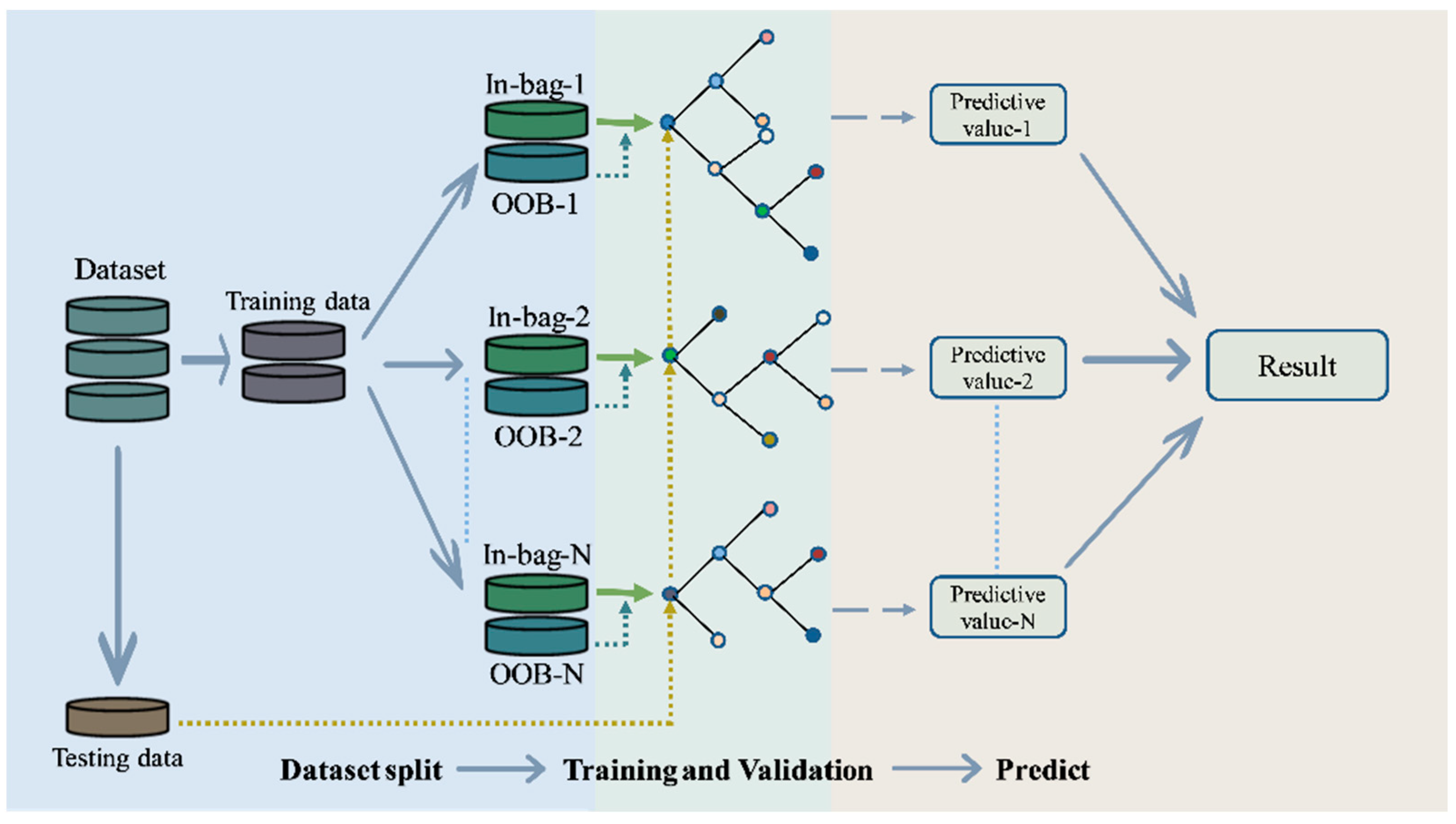
2.4. Random Forest Applications on Image Detection and Driving Force Analysis

Random Forest is a well-established approach in classification and nonlinear regression analysis by creating a collection of classification trees with binary divisions [53]. In this study, the RF model was used for lake surface extraction and driving forces analysis of lake surface area variations in the QHL basin. The RF regression model was constructed using the Random Forest package in the R. The construction of the RF model and the drawing of the partial dependency graph in this paper are all implemented on Rstudio. The specific process of building an RF model is as follows (Figure 2): the training data is sampled N times using bootstrap method, two-thirds of the in-bag data is used as training data, and one-third of the data that has not been sampled is used as out-of-bag (OOB) data. The Cart tree is used as a weak learner, and only the data in the bag is used in the process of building the tree. The features of each node when splitting are generated from some variables randomly selected, and the unbiased error against conventional errors is obtained from the data outside the bag. The above procedure is repeated several times, and the results are then averaged over all trees to obtain the predicted values of the dependent variable. The RF model is used for quantitative analysis of importance, and the nonlinear relationship between the dependent variable and the independent variables is depicted by the partial dependence graph, which enhances the interpretability of the RF model.
In this study, the random forest is used as the research method. The seven bands of Landsat images were input into the RF model as independent variables, while the water and non-water bodies were manually marked as the dependent variables. Then the RF classification model was established to extract the lake area. In the attribution of lake change, an RF regression model, developed with climate factors as independent variables and lake changes as dependent variables, was used to quantify the contribution of each factor to lake area change. The main evaluation metrics of variable importance in the RF model are IncMSE and IncNodePurity. In this paper, IncNodePurity is used as the evaluation index of variable importance. IncNodePurity is the degree of influence of the variable on each decision tree node, and the larger the value, the more important the variable is, and the opposite is relatively unimportant.

3. Results and Analysis

3.1. Lake Area Extraction by RF and Accuracy Evaluation

The RF algorithm has a better extraction effect on the water-sand shore, which can filter out the fine water and effectively separate the sand shore from the large area of lake water to highlight the boundary. According to the comparison of the extracted lake area and actual lake area from TPDC, the relative errors of the six images were all below 1% (Table 1), indicating that the lake-water extraction based on the RF model is feasible. This highlighted the utilization of RF in alpine ecosystems, where the formation and melting of lake ice was one of the unique properties of lakes on the Qinghai-Tibet Plateau.
In this study, observed water levels in the Xiashe hydrological station (36°35′16″N, 100°29′28″E) from 2003 to 2009 were used to verify the validity of ICESat datasets. As illustrated in Figure 3, the proximity between the observed and satellite water levels were characterized by RMSE = 0.099 m, R = 0.933, which indicated that ICESat/GLAS and ICESat-2/ATLAS datasets could accurately measure the water level in the QHL.

3.2. Spatial-Temporal Variations of the QHL

3.2.1. Time Series Characteristics of Lake Change

The long-term time series of the QHL showed obvious phased characteristics in decades. Figure 4 presented the time series of lake storage anomalies from 1987 to 2020. It fluctuated with a slight expansion at the end of the 1980s, causing a 9.84 × 10⁸ m3 storage increase from 1987 to 1989. However, a sharp decrease (−2.58 × 10⁸ m3·yr−1, R2 = 0.86, p < 0.01) occurred from 1989 to 2004, which caused the minimum lake area to appear in 2004 during the past three decades. After 2004, there was a significant increase in lake storage in general with an average increasing rate of 6.92 × 10⁸ m3·yr−1 (R2 = 0.92, p < 0.01). In general, the change of the QHL showed a pattern of “shrinkage–expansion” over the past three decades, which can be divided into two stages, namely, the decreasing stage (from 1987 to 2004) and the increasing stage (from 2004 to 2020), which both comprise 17 years. The turning point occurred in 2004 when the area of the QHL changed significantly, after which the area expanded gradually.

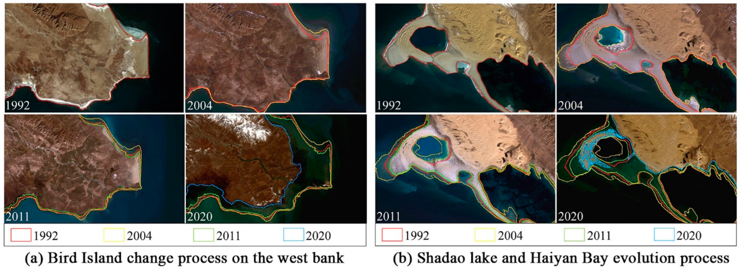
3.2.2. Spatial Characteristics of Lake Change

The phased characteristics of lake change were also reflected in the spatial scale. To investigate the shoreline change of the QHL, the thematic maps based on four Landsat images (1992, 2004, 2011 and 2020) were generated. Figure 5 clearly displayed that the west and east coast of the QHL changed distinctly during the past three decades, especially on Bird Island on the west coast (Figure 5a), and Shadao Island and Haiyan Bay on the east coast (Figure 5b). During the first stage from 1992 to 2004, the extent of water bodies decreased on Bird Island. In addition, decreases in water bodies were also identified in the eastern portions of the QHL. The area of Shadao Lake was significantly reduced, and the surface area of exposed sandy land continued to increase. The long sandbank between Haiyan Bay and the QHL was also significantly enlarged. By 2004, Shadao Lake and Haiyan Bay were almost entirely separated from the main body of the QHL. During the second stage from 2004 to 2011, as the area of the QHL gradually increased, the land shrank inwardly on Bird Island. It is noteworthy that the water bodies of Shadao Lake expanded the most, forming many smaller bodies of water in nearby sandy areas. After 2011, the water area of the QHL showed a significant trend of increasing expansion. Other than that, Shadao Lake and Haiyan Bay were connected to the main body of the QHL by 2020 when the sand bank was completely submerged by water. From a spatial perspective, the QHL has undergone a dynamic process of “slight shrinkage–expansion-rapid expansion” over 34 years.

3.3. Attribution of Variations of the QHL

The reasons for the lake fluctuations can be attributed to climatic and/or anthropogenic factors [35,54,55]. However, water usage by anthropogenic activities only accounts for about 1.8% of the evaporation loss of the lake or 2.5% of the total river discharge, which implied that water usage by anthropogenic activities has not affected the QHL [32]. Hence, climate factors are the major driving forces on lake fluctuation.

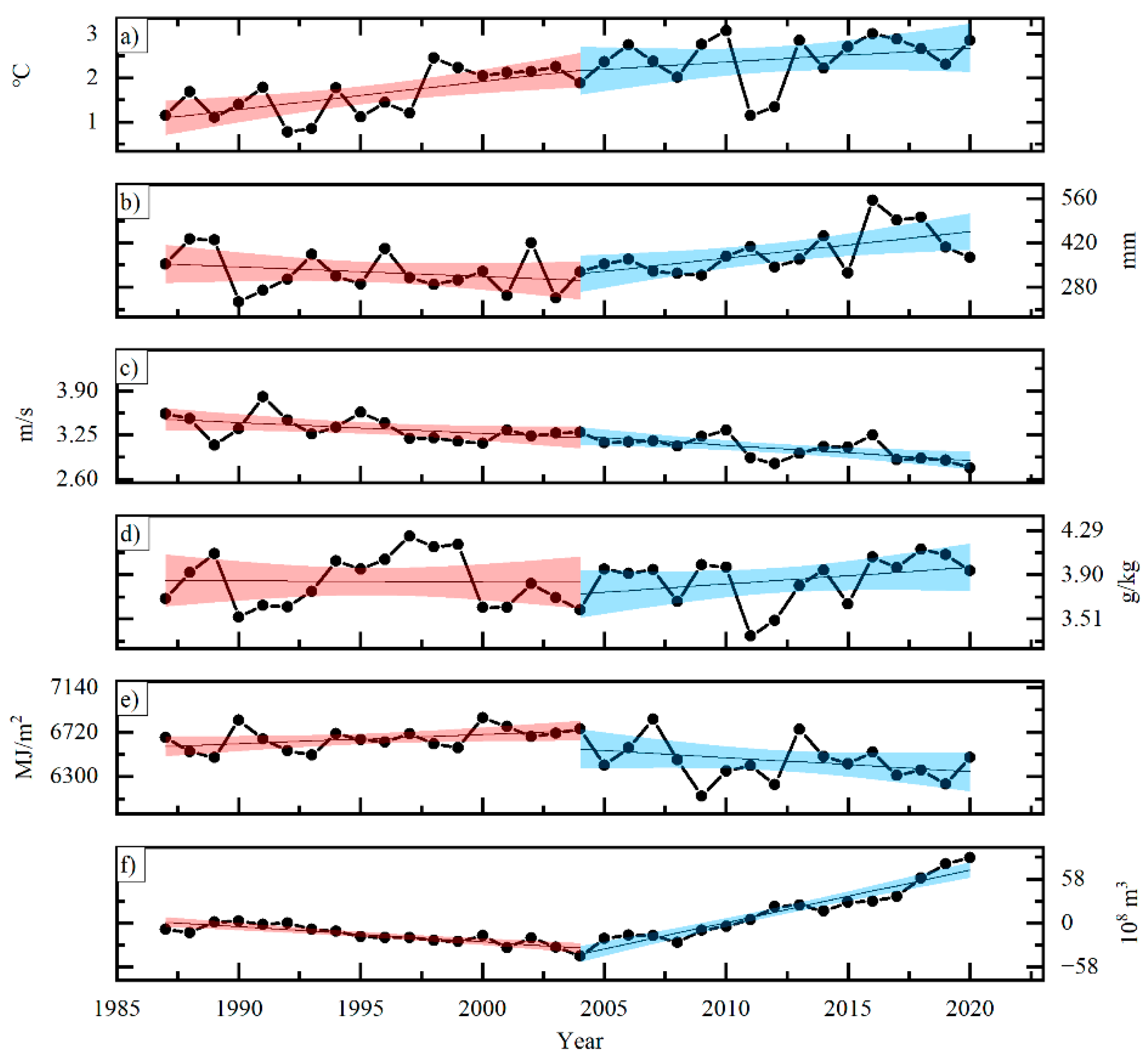
3.3.1. Climate Features of Lake Qinghai from 1987 to 2020

Based on hydrologic balance, temperature, precipitation, radiation, wind speed, and humidity were important climate factors for the lake change. The analyses of climate variations from 1987 to 2020 were as follows. In Figure 6, the annual average temperature of the QHL showed a significantly increasing trend (0.048 °C·yr−1, R2 = 0.51, p < 0.01) from 1987 to 2020. Annual precipitation increased by 3.29 mm·yr−1(R2 = 0.20, p < 0.01). Both wind speed and radiation of the QHL had significantly decreased trends (wind speed: −0.018 m·s−1·yr−1, R2 = 0.60, p < 0.01; radiation: −9.50 MJ·m−2·yr−1, R2 = 0.26, p < 0.01) from 1987 to 2020. The specific humidity increased by 0.21 × 10⁻² g·kg−1·yr−1. In general, obvious warming, humidifying, solar dimming, and wind reduction occurred in the QHL from 1987 to 2020, which affected the variations of the QHL.
According to the turning point of the QHL, we found that climate factors showed different trends before and after 2004. Annual average temperature increased significantly (0.064 °C·yr−1, R2 = 0.39, p < 0.01) before 2004 and weakly (0.032 °C·yr−1, R2 = 0.02) after 2004. Precipitation decreased by −3.08mm·yr−1 before 2004, but significantly increased (8.31 mm·yr−1, R2 = 0.31, p < 0.01) after 2004. Radiation showed a significant increased trend (8.70 MJ·m−2·yr−1, R2 = 0.14, p < 0.1) before 2004 and decreased trend (−13.44 MJ·m−2·yr−1, R2 = 0.06) after 2004. Both the wind speeds before and after 2004 indicated significantly decreased trends with the rates of −0.016 m·s−1·yr−1 (R2 = 0.17, p < 0.1), and −0.022 m·s−1·yr−1 (R2 = 0.40, p < 0.01), respectively. Specific humidity decreased by −0.11 × 10⁻² g·kg−1·yr−1 from 1987 to 2004 and increased by 1.46 × 10⁻² g·kg−1·yr−1 from 2004 to 2020. Generally, obvious warming, drying, and solar brightening were important climate variations for the shrinkage of the QHL before 2004, while warming slowdown, humidifying, accelerating wind reduction, and solar dimming had important associative effects on the expansion of the QHL after 2004.

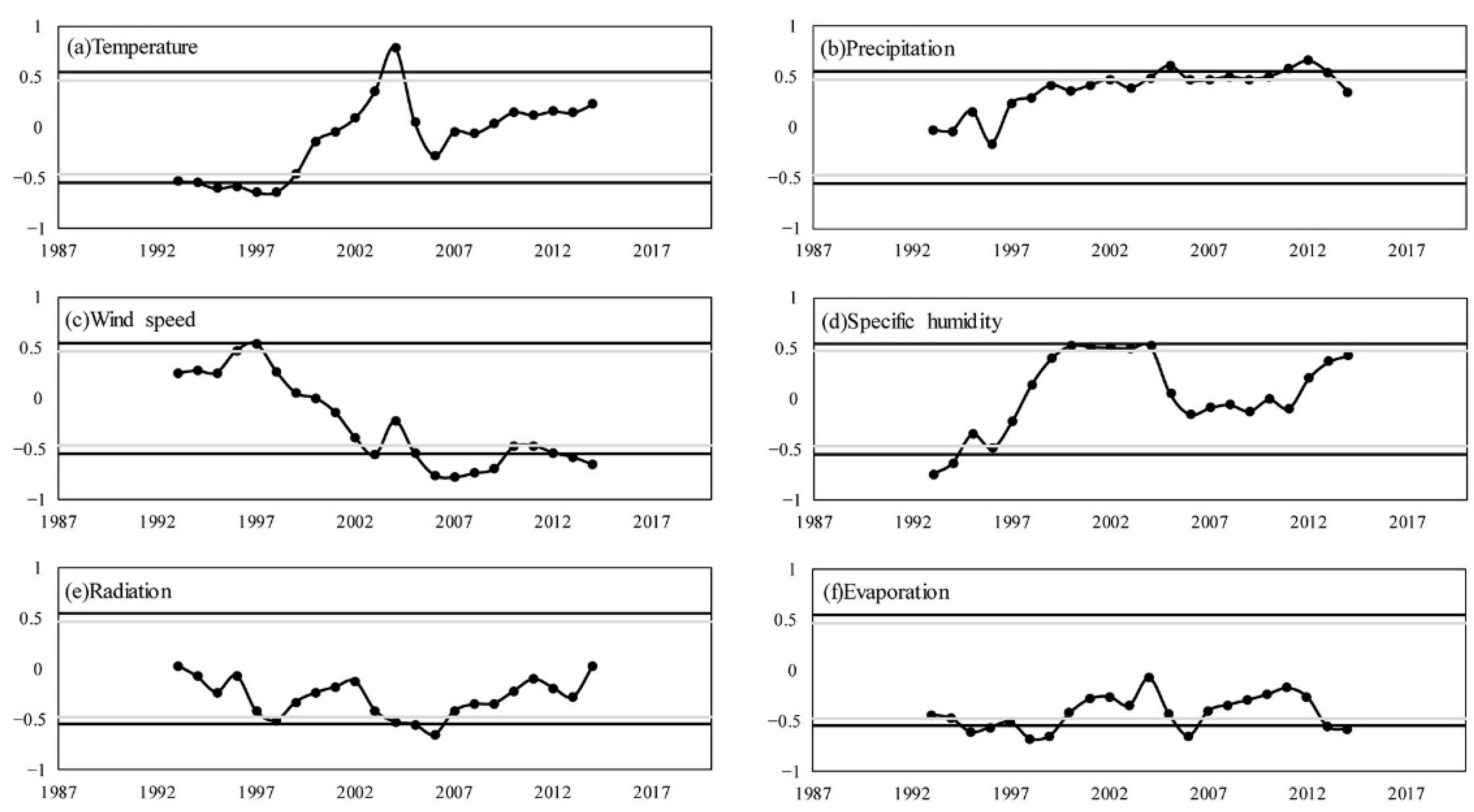
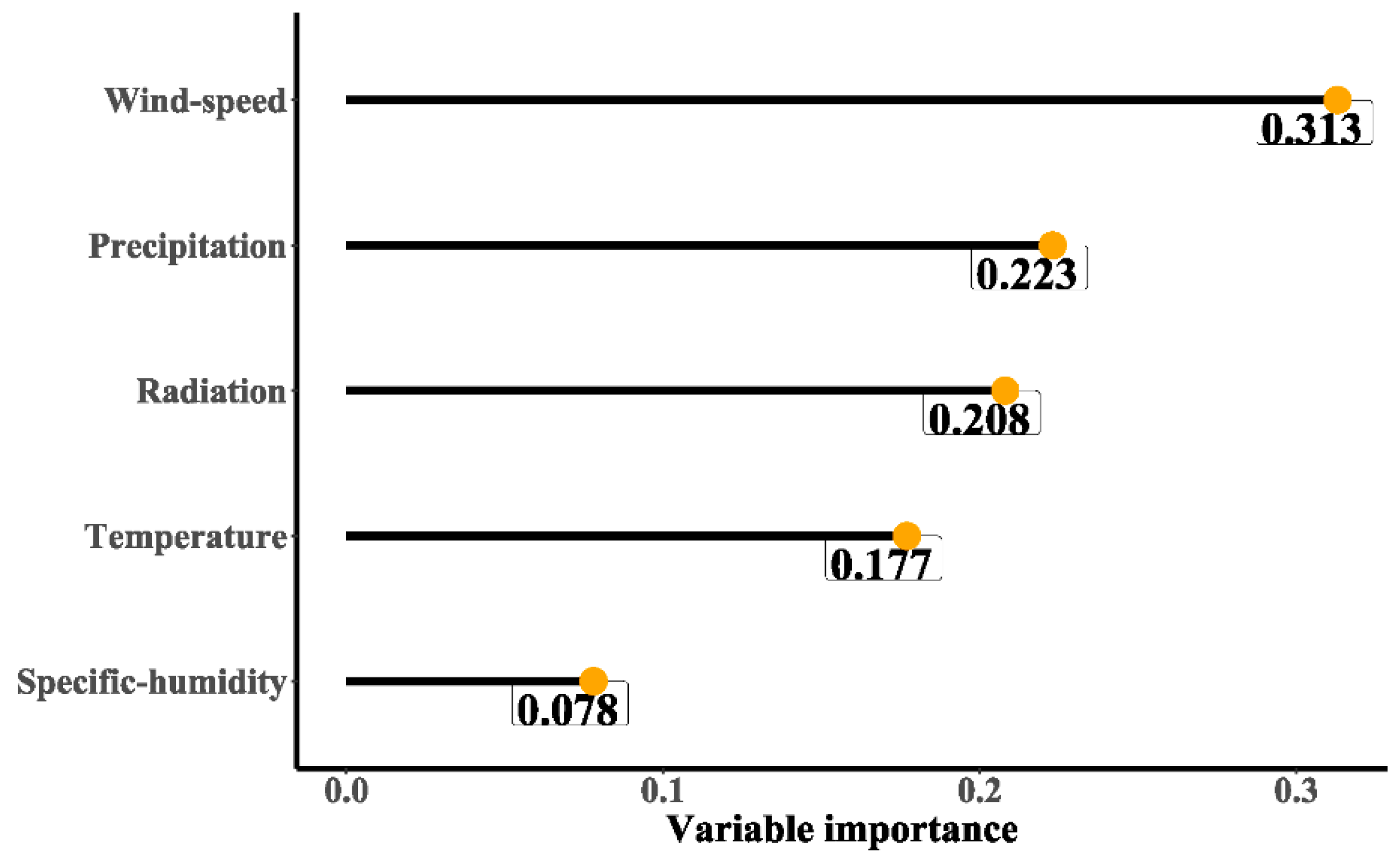
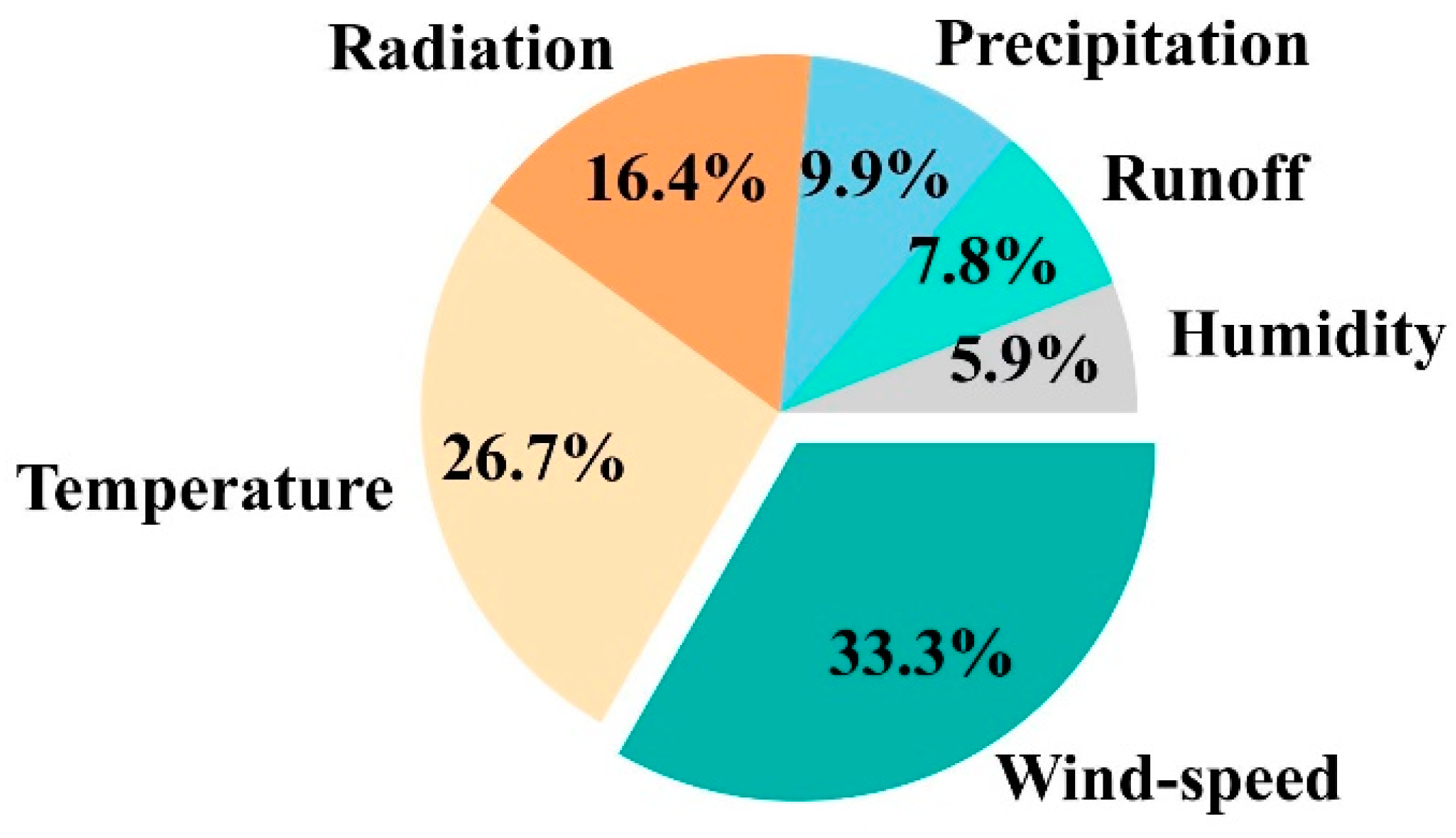
3.3.2. Responses of Lake Change to Climate Variations

Since the phased characteristics were reflected in the variations of lake storage and climate factors, it was necessary to study the phased effects of climate variations on the storage of the QHL. A 13-year sliding correlation analysis was carried out on the variations of lake storage anomaly and climatic factors from 1987 to 2020. As shown in Figure 7a, correlation coefficients between lake storage anomaly and annual average temperature passed a 90% confidence level from 1993 to 1998, which meant that lake storage anomaly was significantly negatively correlated with the annual average temperature from 1987 to 2004. As for precipitation in Figure 7b, a significant correlation (p < 0.05) from 2005 to 2013 meant that precipitation indicated significant positive effects on lake change after 1999. In Figure 7c, a significant correlation (p < 0.05) from 2005 to 2014 indicated significant negative effects of wind speed on the lake change after 1999. In Figure 7d for specific humidity, a significant correlation (p < 0.05) occurred from 2000 to 2004, which indicated that specific humidity had significant positive effects on lake storage from 1994 to 2010. Figure 7e showed that radiation had weakly negative effects on lake change throughout the whole period. In general, temperature dominates lake changes before 2004 by increasing evaporation, while precipitation and wind speed led the lake to change after 1999. Radiation showed continually weak negative effects on the storage of the QHL.
As a direct source of Lake Recharge, precipitation generally showed a positive effect with the change of the lake. Temperature, as a heat indicator, can further influence the change of the QHL area in other ways. Wind speed would not directly affect the change of the lake, but wind speed had a direct connection with lake evaporation. Moreover, evaporation as a direct source of lake loss showed a negative effect on lake area change.
To further quantify the contributions of climate variations to lake change, the RF algorithm was used to rank the importance of the influencing factors and to calculate the contribution of each climate factor. In Figure 8, wind speed, precipitation, radiation, temperature, and specific humidity could explain 31.3%, 22.3%, 20.8%, 17.7% and 7.8% of lake storage changes, respectively. It could be seen that, among climate factors, wind speed played the first dominant role in controlling the storage of the QHL. Precipitation, radiation, and temperature also indicated important weights to the lake change. Combined with the above-phased characteristics of lake change and climate variations, obvious warming led to the shrinkage of the QHL before 2004 through increasing evaporation, while humidifying and accelerating wind reduction, which dominated the expansion of the QHL after 2004 by increasing precipitation and decreasing evaporation.

4. Discussion

4.1. The Advantages of RF in Image Extraction and Driver Identification

A single satellite dataset is insufficient to detect target objects. Previous studies have therefore evaluated the impact of multi-source remote sensing datasets joined with auxiliary geographic datasets such as elevation or soil types to improve the classification accuracy [56]. Several reports have shown that an RF classifier has been used to assess the importance of each data source for the classification results for supervised classification purposes [57,58]. In reviewing the literature, the existing water identification methods are mainly using the threshold and decision rules of different water features. Yet some studies have noted that the RF algorithm especially provides the relative importance of independent variables in the classification model for both overall classification results and each class [59,60,61,62], which gives insight into the classification results of satellite imagery. The current study found that RF was inclined to yield higher accuracy compared to existing parametric classifiers, especially when the data was complex data with a high-dimensional feature space in the transition zone of land and water bodies. In Figure 9, the sand island is located in the northeast of the QHL, which is formed by the lake sand monopoly protruding from the water surface to receive wind and sand accumulation. In addition, the formation and melting of lake ice are two of the unique properties of Qinghai-Tibet Plateau lakes, and the surface of the QHL starts to freeze in winter. In this context, the spectral difference between ice and water is large, while the spectral characteristics of ice and snow are similar. Therefore, thresholds of traditional water feature indices were easy to extract the snow and lake ice on the lake shore at the same time, and further blur the water-land boundary. However, the RF algorithm can avoid the influence of the set threshold value to a certain extent, and the water-land boundary is clearer compared to traditional Normalized Difference Water Index (NDWI). In general, The QHL derived from RF approach had a clearer boundary of water, ice, snow and sand banks, without further consideration of setting threshold by using NDWI.
As mentioned in the literature review, RF can also effectively solve the problems of overfitting and multicollinearity, which have been widely used in data mining, ecology, and other disciplines [20,63,64]. Indeed, RF regression can use the feature combination to include more than one predictor instead of using one predictor for one feature to reduce the high-order interactions. Thus, RF algorithms can assess the relative importance of predictive variables in a model for the global results and each class [53]. In the present research, the quantitative RF analysis showed that dominant factors were wind speed, precipitation, radiation, temperature, and specific humidity in order, explaining 31.3%, 22.3%, 20.8%, 17.7% and 7.8% of lake storage changes of the QHL, respectively. From the perspective of water balance, lake storage changes were decided by evaporation, precipitation, and runoff. Meanwhile, evaporation was mainly determined by wind speed, temperature, and radiation. In addition, river runoff was sensitive to precipitation [65]. Therefore, the lake storage changes were mainly influenced by evaporation and precipitation.

4.2. Driving Mechanism of Precipitation in the QHL: Atmospheric Circulation Perspective

Water vapor transport strongly affects the precipitation in a certain area. The intersection of the East Asian monsoon, the Indian monsoon, and the westerly jet stream affects the QHL [36,39,65], suggesting a complex water vapor interaction. Previous research confirmed that the precipitation of the QHL is highly affected by the variations in atmospheric circulation and is impacted by the interaction of the Westerlies and Asian monsoon [66,67]. A comprehensive analysis of water vapor transport based on the ERA5 monthly dataset (Figure 10) clearly showed that the precipitation in the QHL region was mainly from three transport pathways, which were south and southwest from the Indian monsoon, southeast from the East Asian monsoon, and west from mid-latitude westerlies. Especially, monsoons played key roles in precipitation variation in the QHL. In addition, the temporal heterogeneity of the driving mechanism of water vapor on precipitation led to the phased characteristics of lake storage change. In the present research, weak drying before 2004 and significant humidifying after 2004 in Figure 6 were consistent with the shrinkage–expansion of the QHL during the same periods. Combined with changes in water vapor over the past decades, the decrease in water vapor before 2004 led to the downward trend in precipitation, and the increase in water vapor after 2004 determined the rise in precipitation. In general, variations in water vapor decided precipitation trends, which further affected the lake storage changes in the QHL.
Moreover, the water vapor transport stream exhibits strong interannual variations, which are influenced by large-scale atmospheric circulation such as ENSO (El Niño-Southern Oscillation). From the water vapor analysis in Figure 10, the results showed consistent high and low precipitation over the QHL during the La Nina year (1989) and El Nino years (1994, 1997, and 2004). Most suppressed rainfall patterns were strongly related to the development of El Nino events, with positive SST over the central-eastern equatorial Pacific. Because the Walker circulation was weakened, a weak Asian summer monsoon was producing an atmospheric motion anomaly over the Pacific and Indian Oceans. La Nina events were the opposite of the El Nino events. However, either high or low precipitation did not always occur in ENSO years. For example, when La Nina was not well developed but NAO (North Atlantic oscillation) showed a strong positive phase, precipitation was anomalously high over the QHL region in 2012 and 2018 (Figure 10e,f). Thus, the interaction of the NAO-related Westerlies and ENSO-related Asian Monsoons may trigger anomalous precipitation by driving water vapor transport [68,69], which affected lake changes in the QHL.

4.3. Driving Mechanism of Evaporation in the QHL

For seasonal changes, lake evaporation variability is strongly related to climatic variables, such as land surface temperature, net radiation, and near-surface wind speed. Generally speaking, higher air temperature can result in a higher average kinetic energy for the movement of water molecules and evaporation. However, the fluctuation of evaporation was not coinciding with the continuous increase of air temperature in the QHL especially after 2004. This finding was consistent with those reported that the air temperature increased while the pan evaporation decreased in most regions during the past decades, and this phenomenon is called “the evaporation paradox” [70,71,72]. Here, the RF model was used to quantify climate factors’ contributions to evaporation (Figure 11). As can be seen from Figure 11, wind speed has the highest contribution to evaporation, reaching 33.3% in QHL. Temperature and radiation reported stronger contributions than the other three factors, explaining 26.7% and 16.4% of evaporation changes in the QHL, respectively. In addition, the phased characteristics of lake storage change were determined by the temporal heterogeneity of the driving mechanism of climate change on evaporation. More specifically, the increasing trend in evaporation starting from the 1980s may be more linked to the increasing temperature. On the contrary, the decreasing trend in evaporation starting from 2004 may be related to the declining wind speed and radiation with the warming slowdown in the QHL region. The phased characteristics of evaporation variations determined the shrinkage and expansion of the QHL before and after 2004.
In the present research, we mainly investigated the individual impact of climate factors on the lake changes of the QHL and gave less consideration to the interactions between these factors. In future research, interactions between these factors should be considered to quantify the relative contribution of different driving factors. In addition, extreme atmospheric oscillations, such as ENSO and NAO events, have indicated obvious influences on global climate change in recent decades. This study preliminarily discussed the impact of ENSO and NAO events on water vapor transport in the Qinghai-Tibet Plateau. The influence of atmospheric oscillations on the alpine hydrological cycle requires further analysis in the future.

5. Conclusions

Lake change in the past decades reflects the balance of water mass balance on a basin and is strongly related to climate variables of precipitation, temperature, evaporation, etc. Thus, the expansion and shrinkage of the enclosed lake are sensitive indicators of climate change. In the present research, QHL fluctuated strongly, showing a pattern of shrinkage expansion from 1987 to 2020. The lake storage significantly decreased by −2.58 × 10⁸ m3·yr−1 (R2 = 0.86, p < 0.01) from 1989 to 2004 and sharply increased (6.92 × 10⁸ m3·yr−1, R2 = 0.92, p < 0.01) after 2004. RF analysis indicated that lake storage changes were mainly influenced by evaporation and precipitation. Meanwhile, the temporal heterogeneity of the driving mechanism of climate change led to the phased characteristics of lake storage change. In detail, obvious warming led to the shrinkage of the QHL before 2004 through increasing evaporation, while humidifying and accelerating wind stilling dominated the expansion of the QHL after 2004 by increasing precipitation and decreasing evaporation. The framework presented herein provides accurate detection and monitoring of water bodies at different locations of the Qinghai-Tibet Plateau and provides a necessary basis for further study on the hydrologic process and its response to climate change in alpine regions.

Author Contributions

Conceptualization, W.G.; methodology, W.G. and X.N.; software, Y.M., X.N. and W.G.; formal analysis, W.G. and X.N.; validation, X.N., Y.M. and T.L.; writing—original draft preparation, W.G. and X.N.; writing—review and editing, X.N., T.L., Y.M. and J.Z.; supervision, W.G.; project administration, W.G. and X.N.; funding acquisition, W.G. All authors have read and agreed to the published version of the manuscript.

Funding

This study was financially supported by the 2nd Tibetan Plateau Scientific Expedition and Research (2019QZKK0101), the National Natural Science Foundation of China (42071124), the Fundamental Research Funds for the Central Universities (XZY012019008), and the State Key Laboratory of Loess and Quaternary Geology (SKLLQG1809).

Data Availability Statement

Publicly available datasets were used in this study. The Landsat MSS/TM/ETM images were acquired from the U.S. Geological Survey (USGS) (https://www.usgs.gov/ (accessed on 1 June 2021)). The ICESat/GLAS and ICESat-2/ATLAS datasets were publicly available from the Goddard Space Flight Center (https://icesat.gsfc.nasa.gov/ (accessed on 1 June 2021)). The CMFD was available from the National Tibetan Plateau Data Center (TPDC) (http://data.tpdc.ac.cn/en/ (accessed on 1 June 2021)). ERA5 monthly averaged data on single levels was available from the European Centre for Medium-Range Weather Forecasts (ECMWF) (https://cds.climate.copernicus.eu/ (accessed on 1 June 2022)).

Conflicts of Interest

The authors declare no conflict of interest. The funders had no role in the design of the study; in the collection, analyses, or interpretation of data; in the writing of the manuscript, or in the decision to publish the results.

References

  1. Zhang, L.; Sun, P.; Huettmann, F.; Liu, S. Where Should China Practice Forestry in a Warming World? Glob. Change Biol. 2022, 28, 2461–2475. [Google Scholar] [CrossRef]
  2. Woolway, R.I.; Kraemer, B.M.; Lenters, J.D.; Merchant, C.J.; O’Reilly, C.M.; Sharma, S. Global Lake Responses to Climate Change. Nat. Rev. Earth Env. 2020, 1, 388–403. [Google Scholar] [CrossRef]
  3. Busker, T.; de Roo, A.; Gelati, E.; Schwatke, C.; Adamovic, M.; Bisselink, B.; Pekel, J.-F.; Cottam, A. A Global Lake and Reservoir Volume Analysis Using a Surface Water Dataset and Satellite Altimetry. Hydrol. Earth Syst. Sci. 2019, 23, 669–690. [Google Scholar] [CrossRef] [Green Version]
  4. Yang, K.; Wu, H.; Qin, J.; Lin, C.; Tang, W.; Chen, Y. Recent Climate Changes over the Tibetan Plateau and Their Impacts on Energy and Water Cycle: A Review. Glob. Planet. Change 2014, 112, 79–91. [Google Scholar] [CrossRef]
  5. Moser, K.A.; Baron, J.S.; Brahney, J.; Oleksy, I.A.; Saros, J.E.; Hundey, E.J.; Sadro, S.; Kopáček, J.; Sommaruga, R.; Kainz, M.J.; et al. Mountain Lakes: Eyes on Global Environmental Change. Glob. Planet. Change 2019, 178, 77–95. [Google Scholar] [CrossRef] [Green Version]
  6. Ghasemigoudarzi, P.; Huang, W.; De Silva, O.; Yan, Q.; Power, D. A Machine Learning Method for Inland Water Detection Using CYGNSS Data. IEEE Geosci. Remote Sens. Lett. 2022, 19, 8001105. [Google Scholar] [CrossRef]
  7. Zhang, K.; Shi, H.; Peng, J.; Wang, Y.; Xiong, X.; Wu, C.; Lam, P.K.S. Microplastic Pollution in China’s Inland Water Systems: A Review of Findings, Methods, Characteristics, Effects, and Management. Sci. Total Environ. 2018, 630, 1641–1653. [Google Scholar] [CrossRef] [PubMed]
  8. Zhang, G.; Yao, T.; Piao, S.; Bolch, T.; Xie, H.; Chen, D.; Gao, Y.; O’Reilly, C.M.; Shum, C.K.; Yang, K.; et al. Extensive and Drastically Different Alpine Lake Changes on Asia’s High Plateaus during the Past Four Decades. Geophys. Res. Lett. 2017, 44, 252–260. [Google Scholar] [CrossRef] [Green Version]
  9. Song, C.; Huang, B.; Ke, L. Modeling and Analysis of Lake Water Storage Changes on the Tibetan Plateau Using Multi-Mission Satellite Data. Remote Sens. Environ. 2013, 135, 25–35. [Google Scholar] [CrossRef]
  10. Canaz, S.; Karsli, F.; Guneroglu, A.; Dihkan, M. Automatic Boundary Extraction of Inland Water Bodies Using LiDAR Data. Ocean Coast. Manag. 2015, 118, 158–166. [Google Scholar] [CrossRef]
  11. Qiao, B.; Zhu, L.; Yang, R. Temporal-Spatial Differences in Lake Water Storage Changes and Their Links to Climate Change throughout the Tibetan Plateau. Remote Sens. Environ. 2019, 222, 232–243. [Google Scholar] [CrossRef]
  12. Zhang, G.; Yao, T.; Xie, H.; Yang, K.; Zhu, L.; Shum, C.K.; Bolch, T.; Yi, S.; Allen, S.; Jiang, L.; et al. Response of Tibetan Plateau Lakes to Climate Change: Trends, Patterns, and Mechanisms. Earth-Sci. Rev. 2020, 208, 103269. [Google Scholar] [CrossRef]
  13. Gronewold, A.D.; Stow, C.A. Water Loss from the Great Lakes. Science 2014, 343, 1084–1085. [Google Scholar] [CrossRef] [PubMed]
  14. Zhang, G.; Yao, T.; Shum, C.K.; Yi, S.; Yang, K.; Xie, H.; Feng, W.; Bolch, T.; Wang, L.; Behrangi, A.; et al. Lake Volume and Groundwater Storage Variations in Tibetan Plateau’s Endorheic Basin. Geophys. Res. Lett. 2017, 44, 5550–5560. [Google Scholar] [CrossRef]
  15. Woodcock, C.E.; Loveland, T.R.; Herold, M.; Bauer, M.E. Transitioning from Change Detection to Monitoring with Remote Sensing: A Paradigm Shift. Remote Sens. Environ. 2020, 238, 111558. [Google Scholar] [CrossRef]
  16. Phiri, D.; Simwanda, M.; Salekin, S.; Nyirenda, V.; Murayama, Y.; Ranagalage, M. Sentinel-2 Data for Land Cover/Use Mapping: A Review. Remote Sens. 2020, 12, 2291. [Google Scholar] [CrossRef]
  17. Biancamaria, S.; Lettenmaier, D.P.; Pavelsky, T.M. The SWOT Mission and Its Capabilities for Land Hydrology. Surv. Geophys. 2016, 37, 307–337. [Google Scholar] [CrossRef] [Green Version]
  18. Crétaux, J.-F.; Abarca-del-Río, R.; Bergé-Nguyen, M.; Arsen, A.; Drolon, V.; Clos, G.; Maisongrande, P. Lake Volume Monitoring from Space. Surv. Geophys. 2016, 37, 269–305. [Google Scholar] [CrossRef] [Green Version]
  19. Foody, G.M. Explaining the Unsuitability of the Kappa Coefficient in the Assessment and Comparison of the Accuracy of Thematic Maps Obtained by Image Classification. Remote Sens. Environ. 2020, 239, 111630. [Google Scholar] [CrossRef]
  20. Tyralis, H.; Papacharalampous, G.; Langousis, A. A Brief Review of Random Forests for Water Scientists and Practitioners and Their Recent History in Water Resources. Water 2019, 11, 910. [Google Scholar] [CrossRef] [Green Version]
  21. Feyisa, G.L.; Meilby, H.; Fensholt, R.; Proud, S.R. Automated Water Extraction Index: A New Technique for Surface Water Mapping Using Landsat Imagery. Remote Sens. Environ. 2014, 140, 23–35. [Google Scholar] [CrossRef]
  22. Fisher, A.; Flood, N.; Danaher, T. Comparing Landsat Water Index Methods for Automated Water Classification in Eastern Australia. Remote Sens. Environ. 2016, 175, 167–182. [Google Scholar] [CrossRef]
  23. Hu, T.; Yang, J.; Li, X.; Gong, P. Mapping Urban Land Use by Using Landsat Images and Open Social Data. Remote Sens. 2016, 8, 151. [Google Scholar] [CrossRef]
  24. Rokni, K.; Ahmad, A.; Selamat, A.; Hazini, S. Water Feature Extraction and Change Detection Using Multitemporal Landsat Imagery. Remote Sens. 2014, 6, 4173–4189. [Google Scholar] [CrossRef] [Green Version]
  25. Du, Y.; Zhang, Y.; Ling, F.; Wang, Q.; Li, W.; Li, X. Water Bodies’ Mapping from Sentinel-2 Imagery with Modified Normalized Difference Water Index at 10-m Spatial Resolution Produced by Sharpening the SWIR Band. Remote Sens. 2016, 8, 354. [Google Scholar] [CrossRef] [Green Version]
  26. Maxwell, A.E.; Warner, T.A.; Fang, F. Implementation of Machine-Learning Classification in Remote Sensing: An Applied Review. Int. J. Remote Sens. 2018, 39, 2784–2817. [Google Scholar] [CrossRef] [Green Version]
  27. Markus, T.; Neumann, T.; Martino, A.; Abdalati, W.; Brunt, K.; Csatho, B.; Farrell, S.; Fricker, H.; Gardner, A.; Harding, D.; et al. The Ice, Cloud, and Land Elevation Satellite-2 (ICESat-2): Science Requirements, Concept, and Implementation. Remote Sens. Environ. 2017, 190, 260–273. [Google Scholar] [CrossRef]
  28. Ma, Y.; Xu, N.; Liu, Z.; Yang, B.; Yang, F.; Wang, X.H.; Li, S. Satellite-Derived Bathymetry Using the ICESat-2 Lidar and Sentinel-2 Imagery Datasets. Remote Sens. Environ. 2020, 250, 112047. [Google Scholar] [CrossRef]
  29. Yu, G.; Lai, G.; Xue, B.; Liu, X.; Wang, S.; Wang, A. Preliminary Study on the Responses of Lake Water from the Western China to Climate Change in the Future: Monte Carlo Analysis Applied in GCM Simulations and Lake Water Changes. Sci. Limnol. Sin. 2004, 16, 193–202. [Google Scholar]
  30. Dong, C.; Wang, N.; Li, Z.; Yang, P. Forecast of Lake Level in Lake Qinghai Based on Energy-Water Balance Model. Hupo Kexue 2009, 21, 587–593. [Google Scholar]
  31. Cui, B.-L.; Li, X.-Y. The Impact of Climate Changes on Water Level of Qinghai Lake in China over the Past 50 Years. Hydrol. Res. 2016, 47, 532–542. [Google Scholar] [CrossRef] [Green Version]
  32. Yang, G.; Zhang, M.; Xie, Z.; Li, J.; Ma, M.; Lai, P.; Wang, J. Quantifying the Contributions of Climate Change and Human Activities to Water Volume in Lake Qinghai, China. Remote Sens. 2021, 14, 99. [Google Scholar] [CrossRef]
  33. Wang, X.; Liang, T.; Xie, H.; Huang, X.; Lin, H. Climate-Driven Changes in Grassland Vegetation, Snow Cover, and Lake Water of the Qinghai Lake Basin. J. Appl. Remote Sens. 2016, 10, 036017. [Google Scholar] [CrossRef]
  34. Tang, L.; Duan, X.; Kong, F.; Zhang, F.; Zheng, Y.; Li, Z.; Mei, Y.; Zhao, Y.; Hu, S. Influences of Climate Change on Area Variation of Qinghai Lake on Qinghai-Tibetan Plateau since 1980s. Sci. Rep. 2018, 8, 7331. [Google Scholar] [CrossRef] [PubMed] [Green Version]
  35. Dong, H.; Song, Y.; Zhang, M. Hydrological Trend of Qinghai Lake over the Last 60 Years: Driven by Climate Variations or Human Activities? J. Water Clim. Change 2019, 10, 524–534. [Google Scholar] [CrossRef]
  36. Fan, C.; Song, C.; Li, W.; Liu, K.; Cheng, J.; Fu, C.; Chen, T.; Ke, L.; Wang, J. What Drives the Rapid Water-Level Recovery of the Largest Lake (Qinghai Lake) of China over the Past Half Century? J. Hydrol. 2021, 593, 125921. [Google Scholar] [CrossRef]
  37. Gao, Y.; Zhou, X.; Wang, Q.; Wang, C.; Zhan, Z.; Chen, L.; Yan, J.; Qu, R. Vegetation Net Primary Productivity and Its Response to Climate Change during 2001–2008 in the Tibetan Plateau. Sci. Total Environ. 2013, 444, 356–362. [Google Scholar] [CrossRef] [PubMed]
  38. Huang, K.; Zhang, Y.; Zhu, J.; Liu, Y.; Zu, J.; Zhang, J. The Influences of Climate Change and Human Activities on Vegetation Dynamics in the Qinghai-Tibet Plateau. Remote Sens. 2016, 8, 876. [Google Scholar] [CrossRef] [Green Version]
  39. Cui, B.-L.; Xiao, B.; Li, X.-Y.; Wang, Q.; Zhang, Z.-H.; Zhan, C.; Li, X.-D. Exploring the Geomorphological Processes of Qinghai Lake and Surrounding Lakes in the Northeastern Tibetan Plateau, Using Multitemporal Landsat Imagery (1973–2015). Glob. Planet. Change 2017, 152, 167–175. [Google Scholar] [CrossRef] [Green Version]
  40. Tian, P.; Lu, H.; Feng, W.; Guan, Y.; Xue, Y. Large Decrease in Streamflow and Sediment Load of Qinghai–Tibetan Plateau Driven by Future Climate Change: A Case Study in Lhasa River Basin. Catena 2020, 187, 104340. [Google Scholar] [CrossRef]
  41. Xia, M.; Jia, K.; Zhao, W.; Liu, S.; Wei, X.; Wang, B. Spatio-Temporal Changes of Ecological Vulnerability across the Qinghai-Tibetan Plateau. Ecol. Indic. 2021, 123, 107274. [Google Scholar] [CrossRef]
  42. Chen, H.; Zhu, Q.; Peng, C.; Wu, N.; Wang, Y.; Fang, X.; Gao, Y.; Zhu, D.; Yang, G.; Tian, J.; et al. The Impacts of Climate Change and Human Activities on Biogeochemical Cycles on the Qinghai-Tibetan Plateau. Glob. Change Biol. 2013, 19, 2940–2955. [Google Scholar] [CrossRef] [PubMed]
  43. Dong, S.; Shang, Z.; Gao, J.; Boone, R.B. Enhancing Sustainability of Grassland Ecosystems through Ecological Restoration and Grazing Management in an Era of Climate Change on Qinghai-Tibetan Plateau. Agric. Ecosyst. Environ. 2020, 287, 106684. [Google Scholar] [CrossRef]
  44. Pickens, A.H.; Hansen, M.C.; Hancher, M.; Stehman, S.V.; Tyukavina, A.; Potapov, P.; Marroquin, B.; Sherani, Z. Mapping and Sampling to Characterize Global Inland Water Dynamics from 1999 to 2018 with Full Landsat Time-Series. Remote Sens. Environ. 2020, 243, 111792. [Google Scholar] [CrossRef]
  45. Cooley, S.W.; Ryan, J.C.; Smith, L.C. Human Alteration of Global Surface Water Storage Variability. Nature 2021, 591, 78–81. [Google Scholar] [CrossRef]
  46. O’Reilly, C.M.; Sharma, S.; Gray, D.K.; Hampton, S.E.; Read, J.S.; Rowley, R.J.; Schneider, P.; Lenters, J.D.; McIntyre, P.B.; Kraemer, B.M.; et al. Rapid and Highly Variable Warming of Lake Surface Waters around the Globe. Geophys. Res. Lett. 2015, 42, 6235. [Google Scholar] [CrossRef] [Green Version]
  47. Sheykhmousa, M.; Mahdianpari, M.; Ghanbari, H.; Mohammadimanesh, F.; Ghamisi, P.; Homayouni, S. Support Vector Machine Versus Random Forest for Remote Sensing Image Classification: A Meta-Analysis and Systematic Review. IEEE J. Sel. Top. Appl. Earth Obs. Remote Sens. 2020, 13, 6308–6325. [Google Scholar] [CrossRef]
  48. Chang, Z.; Du, Z.; Zhang, F.; Huang, F.; Chen, J.; Li, W.; Guo, Z. Landslide Susceptibility Prediction Based on Remote Sensing Images and GIS: Comparisons of Supervised and Unsupervised Machine Learning Models. Remote Sens. 2020, 12, 502. [Google Scholar] [CrossRef] [Green Version]
  49. Pan, S.; Pan, N.; Tian, H.; Friedlingstein, P.; Sitch, S.; Shi, H.; Arora, V.K.; Haverd, V.; Jain, A.K.; Kato, E.; et al. Evaluation of Global Terrestrial Evapotranspiration Using State-of-the-Art Approaches in Remote Sensing, Machine Learning and Land Surface Modeling. Hydrol. Earth Syst. Sci. 2020, 24, 1485–1509. [Google Scholar] [CrossRef] [Green Version]
  50. Khazaei, B.; Khatami, S.; Alemohammad, S.H.; Rashidi, L.; Wu, C.; Madani, K.; Kalantari, Z.; Destouni, G.; Aghakouchak, A. Climatic or Regionally Induced by Humans? Tracing Hydro-Climatic and Land-Use Changes to Better Understand the Lake Urmia Tragedy. J. Hydrol. 2019, 569, 203–217. [Google Scholar] [CrossRef]
  51. Sauber, J. Ice Elevations and Surface Change on the Malaspina Glacier, Alaska. Geophys. Res. Lett. 2005, 32, L23S01. [Google Scholar] [CrossRef] [Green Version]
  52. Xu, J. Mathematical Methods in Contemporary Geography; Higher Education Press: Beijing, China, 2002. [Google Scholar]
  53. Breiman, L. Random Forests. Mach. Learn. 2001, 45, 5–32. [Google Scholar] [CrossRef] [Green Version]
  54. Chang, B.; He, K.; Li, R.; Sheng, Z.; Wang, H. Linkage of Climatic Factors and Human Activities with Water Level Fluctuations in Qinghai Lake in the Northeastern Tibetan Plateau, China. Water 2017, 9, 552. [Google Scholar] [CrossRef] [Green Version]
  55. Dong, H.; Song, Y. Shrinkage History of Lake Qinghai and Causes during the Last 52 Years. In Proceedings of the 2011 International Symposium on Water Resource and Environmental Protection (ISWREP), Xi’an, China, 20–22 May 2011; pp. 446–449. [Google Scholar]
  56. Kumar, U.; Dasgupta, A.; Mukhopadhyay, C.; Ramachandra, T.V. Examining the Effect of Ancillary and Derived Geographical Data on Improvement of Per-Pixel Classification Accuracy of Different Landscapes. J. Indian Soc. Remote Sens. 2018, 46, 407–422. [Google Scholar] [CrossRef]
  57. Dong, L.; Du, H.; Mao, F.; Han, N.; Li, X.; Zhou, G.; Zhu, D.; Zheng, J.; Zhang, M.; Xing, L.; et al. Very High Resolution Remote Sensing Imagery Classification Using a Fusion of Random Forest and Deep Learning Technique—Subtropical Area for Example. IEEE J. Sel. Top. Appl. Earth Obs. Remote Sens. 2020, 13, 113–128. [Google Scholar] [CrossRef]
  58. Loozen, Y.; Rebel, K.T.; de Jong, S.M.; Lu, M.; Ollinger, S.V.; Wassen, M.J.; Karssenberg, D. Mapping Canopy Nitrogen in European Forests Using Remote Sensing and Environmental Variables with the Random Forests Method. Remote Sens. Environ. 2020, 247, 111933. [Google Scholar] [CrossRef]
  59. Nandlall, S.D.; Millard, K. Quantifying the Relative Importance of Variables and Groups of Variables in Remote Sensing Classifiers Using Shapley Values and Game Theory. IEEE Geosci. Remote Sens. Lett. 2020, 17, 42–46. [Google Scholar] [CrossRef]
  60. Grömping, U. Variable Importance Assessment in Regression: Linear Regression versus Random Forest. Am. Stat. 2009, 63, 308–319. [Google Scholar] [CrossRef]
  61. Genuer, R.; Poggi, J.-M.; Tuleau-Malot, C. Variable Selection Using Random Forests. Pattern Recognit. Lett. 2010, 31, 2225–2236. [Google Scholar] [CrossRef] [Green Version]
  62. Fernandez, D.; Lopez, R.; Briceno, N.; Lopez, J.; Oliva, M. Dynamics of the Burlan and Pomacochas Lakes Using SAR Data in GEE, Machine Learning Classifiers, and Regression Methods. ISPRS Int. J. Geo-Inf. 2022, 11, 534. [Google Scholar] [CrossRef]
  63. Tariq, A.; Shu, H.; Siddiqui, S.; Munir, I.; Sharifi, A.; Li, Q.; Lu, L. Spatio-Temporal Analysis of Forest Fire Events in the Margalla Hills, Islamabad, Pakistan Using Socio-Economic and Environmental Variable Data with Machine Learning Methods. J. For. Res. 2022, 33, 183–194. [Google Scholar] [CrossRef]
  64. Were, K.; Bui, D.T.; Dick, Ø.B.; Singh, B.R. A Comparative Assessment of Support Vector Regression, Artificial Neural Networks, and Random Forests for Predicting and Mapping Soil Organic Carbon Stocks across an Afromontane Landscape. Ecol. Indic. 2015, 52, 394–403. [Google Scholar] [CrossRef]
  65. Cui, B.-L.; Li, X.-Y. Runoff Processes in the Qinghai Lake Basin, Northeast Qinghai-Tibet Plateau, China: Insights from Stable Isotope and Hydrochemistry. Quat. Int. 2015, 380–381, 123–132. [Google Scholar] [CrossRef]
  66. Chow, K.C.; Tong, H.-W.; Chan, J.C.L. Water Vapor Sources Associated with the Early Summer Precipitation over China. Clim. Dyn. 2008, 30, 497–517. [Google Scholar] [CrossRef]
  67. An, Z.; Colman, S.M.; Zhou, W.; Li, X.; Brown, E.T.; Jull, A.J.T.; Cai, Y.; Huang, Y.; Lu, X.; Chang, H.; et al. Interplay between the Westerlies and Asian Monsoon Recorded in Lake Qinghai Sediments since 32 Ka. Sci. Rep. 2012, 2, 619. [Google Scholar] [CrossRef] [Green Version]
  68. Yang, P.; Xia, J.; Zhan, C.; Zhang, Y.; Hu, S. Discrete Wavelet Transform-Based Investigation into the Variability of Standardized Precipitation Index in Northwest China during 1960–2014. Appl. Clim. 2018, 132, 167–180. [Google Scholar] [CrossRef]
  69. Ding, Z.; Lu, R.; Liu, C.; Duan, C. Temporal Change Characteristics of Climatic and Its Relationships with Atmospheric Circulation Patterns in Qinghai Lake Basin. Adv. Earth Sci. 2018, 33, 281–292. [Google Scholar]
  70. Huang, H.; Han, Y.; Cao, M.; Song, J.; Xiao, H.; Cheng, W. Spatiotemporal Characteristics of Evapotranspiration Paradox and Impact Factors in China in the Period of 1960–2013. Adv. Meteorol. 2015, 2015, 519207. [Google Scholar] [CrossRef] [Green Version]
  71. Wang, T.; Zhang, J.; Sun, F.; Liu, W. Pan Evaporation Paradox and Evaporative Demand from the Past to the Future over China: A Review. WIREs Water 2017, 4, 1207. [Google Scholar] [CrossRef]
  72. Wang, H.; Zhang, M.; Cui, L. Evaporation Paradox and Its Mechanism in Coastal Wetlands of Northern China. Mausam 2020, 71, 125–132. [Google Scholar]
Figure 1. Map and location of the QHL. Red Rectangle A represents Bird Island on the west coast, while Red Rectangle B covers Shadao Island and Haiyan Bay on the east coast of the QHL. Yellow triangle is the Xiashe hydrological station. Blue area in the sub-figure (upper right) represents the location of the QHL in the Qinghai-Tibet Plateau.
Remotesensing 15 01144 g001
Figure 2. Theory of Random Forest Algorithm.
Remotesensing 15 01144 g002
Figure 3. Observed water level vs. ICESat water level in the Xiashe hydrological station from 2003 to 2009. RMSE = 0.099 m; R = 0.933.
Remotesensing 15 01144 g003
Figure 4. The time series change of the QHL storage anomaly from 1987 to 2020.
Remotesensing 15 01144 g004
Figure 5. Shoreline change detection using Landsat images from 1992 to 2020.
Remotesensing 15 01144 g005
Figure 6. The variation of climate factors and lake area in Qinghai Basin during the period from 1987 to 2020. (a) average annual air temperature, (b) annual total precipitation, (c) average annual wind speed, (d) average annual specific humidity, (e) annual radiation, (f) lake storage anomaly. The pink area for 1987 to 2004, and the blue area for 2004 to 2020. The dashed lines are linear trends, respectively.
Remotesensing 15 01144 g006
Figure 7. The 13-year sliding Correlation coefficients between lake storage anomaly and climatic factors ((a): Temperature; (b): Precipitation; (c): Wind speed; (d): Specific humidity; (e): Radiation; (f): Evaporation). The gray and black lines denote correlation required for significance at the 90% and 95% levels, respectively.
Remotesensing 15 01144 g007
Figure 8. Random forest variable importance rankings. A higher value indicates the importance of that climate factor in lake change. Removal of that factor causes the model to lose accuracy in prediction.
Remotesensing 15 01144 g008
Figure 9. Lake Boundary extraction comparisons between NDWI (a,c) and RF (b,d).
Remotesensing 15 01144 g009
Figure 10. Anomaly distribution of vertically integrated summer water vapor in (a) 1989, (b) 1994, (c) 1997, (d) 2004, (e) 2012, and (f) 2018. The arrows represented water vapor transport. The red star showed the location of the QHL.
Remotesensing 15 01144 g010
Figure 11. Importance of climate factors on evaporation based on RF in QHL.
Remotesensing 15 01144 g011
Table 1. Accuracy of extracted lakes based on the RF model.
Sensor TypeDateExtracted Lake Area (km²)Actual Lake Area (km²)Relative Error (%)
TM2 October 19874282.6934303.219−0.48
TM5 October 20004233.8034253.22−0.46
TM17 October 20104267.2734251.0580.38
OLI15 October 20154342.094369.499−0.63
OLI5 November 20174404.2924380.2070.55
OLI11 November 20194484.5234468.10.37
The area of the lake here does not include the area of Gahai, a sub-lake on the east side of the QHL.
Disclaimer/Publisher’s Note: The statements, opinions and data contained in all publications are solely those of the individual author(s) and contributor(s) and not of MDPI and/or the editor(s). MDPI and/or the editor(s) disclaim responsibility for any injury to people or property resulting from any ideas, methods, instructions or products referred to in the content.

