UAS-Based Real-Time Detection of Red-Cockaded Woodpecker Cavities in Heterogeneous Landscapes Using YOLO Object Detection Algorithms

Abstract

In recent years, deep learning-based approaches have proliferated across a variety of ecological studies. Inspired by deep learning’s emerging prominence as the preferred tool for analyzing wildlife image datasets, this study employed You Only Look Once (YOLO), a single-shot, real-time object detection algorithm, to effectively detect cavity trees of Red-cockaded Woodpeckers or RCW (Dryobates borealis). In spring 2022, using an unmanned aircraft system (UAS), we conducted presence surveys for RCW cavity trees within a 1264-hectare area in the Sam Houston National Forest (SHNF). Additionally, known occurrences of RCW cavity trees outside the surveyed area were aerially photographed, manually annotated, and used as a training dataset. Both YOLOv4-tiny and YOLOv5n architectures were selected as target models for training and later used for inferencing separate aerial photos from the study area. A traditional survey using the pedestrian methods was also conducted concurrently and used as a baseline survey to compare our new methods. Our best-performing model generated an mAP (mean Average Precision) of 95% and an F1 score of 85% while maintaining an inference speed of 2.5 frames per second (fps). Additionally, five unique cavity trees were detected using our model and UAS approach, compared with one unique detection using traditional survey methods. Model development techniques, such as preprocessing images with tiling and Sliced Aided Hyper Inferencing (SAHI), proved to be critical components of improved detection performance. Our results demonstrated the two YOLO architectures with tiling and SAHI strategies were able to successfully detect RCW cavities in heavily forested, heterogenous environments using semi-automated review. Furthermore, this case study represents progress towards eventual real-time detection where wildlife managers are targeting small objects. These results have implications for more achievable conservation goals, less costly operations, a safer work environment for personnel, and potentially more accurate survey results in environments that are difficult using traditional methods.

1. Introduction

The incorporation of advanced image processing techniques into wildlife monitoring is a rapidly growing trend in ecological studies, among which deep learning has become a standout tool for automating monitoring efforts [1,2,3]. The use of automation to analyze large UAS-derived image datasets is enabling wildlife survey efforts in ways previously unachievable [4,5,6]. Most notably, monitoring regimes drastically reduce the personnel hours necessary to perform image reviews or real-time observations when using deep learning as an alternative [7]. Recent examples of its use span numerous major wildlife taxon [8,9,10], and study objectives include simple identification [9], species classification [11], and wildlife census [12]. Image acquisition was performed with a variety of methods, such as game cameras [13], manned aircraft [7], satellite imageries [10,12], and unmanned aerial systems (UAS) [9,14].

Deep learning, a subcategory of machine learning (ML), identifies data representation using techniques such as convolutional neural networks (CNN). These networks are composed of multiple layers, with each layer leveraging learning from previous ones during model training [15,16,17]. Deep CNNs are designed to learn spatial hierarchies of features automatically and adaptively in complex image datasets where multiple levels of abstraction are present [15]. Studies using region-based, two-step deep learning model architectures, such as R-CNN (Regions with CNN) or Faster R-CNN, have proven to perform accurately but produce relatively slow detections [18]. Deploying a deep learning-based computer vision model in real-time presents practical challenges, such as demanding memory and processing power during training and long detection times at inference. In contrast, single-shot detector models, including You Only Look Once (YOLO), are rapidly gaining popularity in real-time object detection because of their relatively fast inferencing time and exceptional detection performance [18]. As the name suggests, YOLO requires only a single forward propagation pass through the neural network for the entire detection pipeline [18]. Despite the excellent small-object detection ability [19,20,21], the use of YOLO model architectures in wildlife monitoring remains underrepresented. A few recent examples include the use of YOLOv5 for detecting Siberian Cranes [22] and YOLOv4 for bird detection around wind turbines [23]. The real-time detection of wildlife using YOLO models has also seen some progress in the context of large image objects [24] or non-aerial image acquisition [25].

We identified that previous studies often addressed wildlife detection in homogeneous environments [12], targeted large wildlife objects [11], or used image processing techniques that are inappropriate for real-time detection [8,10,26]. Therefore, we sought to assimilate previous work toward real-time detection of small wildlife objects in heterogeneous environments in a manner that demonstrated the entire spectrum of survey methodology, from image acquisition to survey results. UAS-based image capture approaches are becoming increasingly prevalent because of their cost-effectiveness, temporal flexibility, and ability to make high-resolution observations [5,6,27]. Specifically, UAS sensors can observe at less than 2.5 cm per pixel resolution in some configurations and, therefore, possess the most potential for the non-invasive detection of small wildlife in complex, heterogeneous environments [26,28]. For these reasons, we determined a UAS-based approach was most appropriate for our study’s objectives.

Our proposed methods leveraged UAS-based image acquisition and processed the images using single-shot deep learning model architectures of YOLOv4 and YOLOv5, tiling during preprocessing, and Sliced Aided Hyper Inferencing (SAHI) during model testing in the case of YOLOv5. Tiling is an automated preprocessing step that negates time-intensive or overly complex manual preprocessing of images by partitioning a larger parent image into smaller tiles. When tiles mimic model input dimensions, loss of image object detail to compression is eliminated, which can boost small-object detection accuracy by as much as 20% [29]. SAHI, a recent emerging technique, further enables small-object detection by automating tile overlap during inferencing [30]. Tile overlap enables the detection of fringe image objects that might otherwise be split by tiles. A recent study demonstrated that SAHI increased average precision by approximately 5.7% for three different predictors after model tuning [30].

As a case study, we used our trained model to enable presence surveys for RCW cavity trees in areas that were challenging using current methods outlined in the RCW Recovery Plan [31]. Difficult conditions constituted thick midstory vegetation that made navigation and observations from the forest floor difficult to impossible during pedestrian surveys. The excavation of cavities into living pine trees is a unique characteristic of the RCW [32,33], along with bark scaling and resin-well production to deter predators [34]. These characteristics served as our visual cues when labeling image objects. Before any image collection, we performed an intensive review of studies that describe how to mitigate disturbances to wildlife when surveying with a UAS [35,36,37]. After collecting and labeling a total of 978 training sample images, we developed two cavity tree detection models based on YOLOv4 and YOLOv5. Both were then used to infer and review a separate UAS aerial survey conducted on the SHNF near New Waverly, Texas, in the United States. The concurrent use of pedestrian survey methods in the same study area provided baseline survey results for comparison. Our primary goals were to develop new methods for detecting RCW cavities that could enhance current survey protocols in difficult environments. Furthermore, we sought to make progress toward the eventual real-time detection of cavities and convey how our techniques might be applied to other small-object detection problems.

2. Materials and Methods

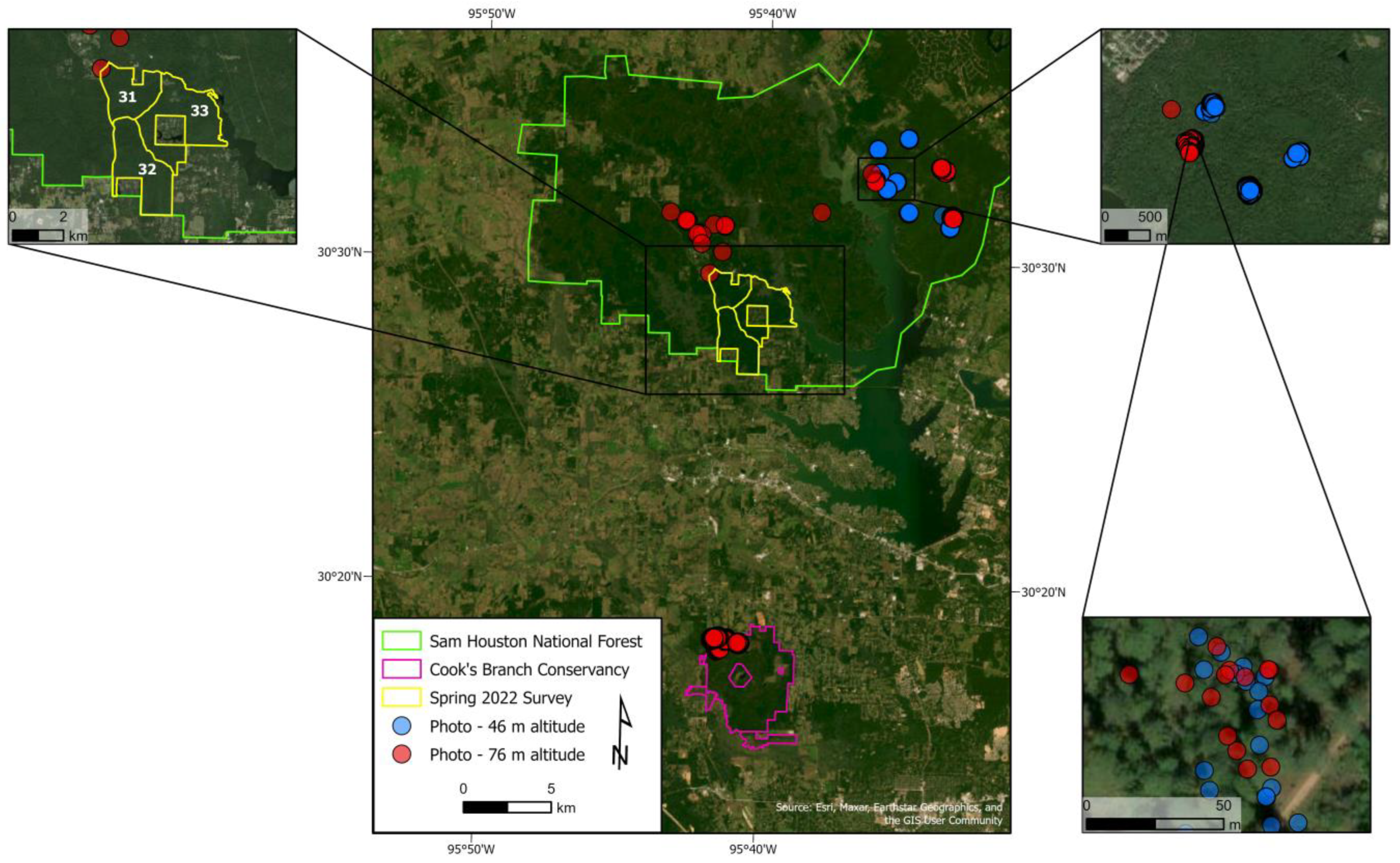
2.1. Study Area

Training sample photos were collected at Cook’s Branch Conservancy (CBC) and the SHNF in spring 2022 (Figure 1). The SHNF is one of the four Forest Service districts in Texas, with 65,978 hectares of public land spanning the Walker, San Jacinto, and Montgomery counties. The RCW population there is relatively large, with over 240 breeding groups. CBC is a privately owned, 2900-hectare wildlife conservation area located in Montgomery County, Texas. For over twenty years, it has undergone a management regime to support a current RCW population of 29 groups.

For both the survey sites, the forest type was predominantly mature loblolly pine (Pinus taeda) mixed with varying levels of mature shortleaf pine (Pinus echinata). RCW habitat is characterized by upland, mature pine, so hardwood species were present but sparse [31,39]. Levels of woody midstory vegetation varied from minimal with grassy openness to dense thickets of yaupon holly (Ilex vomitoria), American sweetgum (Liquidambar styraciflua), and American beautyberry (Callicarpa americana).

Surveying for new RCW trees was conducted in spring 2022 in Compartments 31–33 (1264 hectares) on SHNF (Figure 1). The survey area had very similar defining qualities to the areas where training samples were collected, except that the dense midstory conditions described above were ubiquitous. Despite that, several active RCW groups were present within the study area, along with suitable nesting habitats in unoccupied areas. Following the RCW Recovery Plan, we defined suitable nesting habitat as pine stands above 60 years old and within 0.8 km of suitable foraging habitat [31].

2.2. Training Samples

2.2.1. Training Sample Image Collection

Aerial images were collected with two types of UAS vehicles, a DJI Mavic Pro Platinum and a DJI Mavic 2 Pro (

Table 1. Details on the two UAS vehicles used to capture cavity tree images. In spring 2022, training sample photos were captured at SHNF and CBC in Walker County and Montgomery County, Texas.

Model	DJI Mavic Pro Platinum	DJI Mavic Pro 2
Weight	734 g	907 g
Flight time	30 m	31 m
Sensor	1/2.3″(CMOS)	1″(CMOS)
Effective pixels	12.35 million	20 million
Lens	FOV 78.8°, 26 mm (35 mm format equivalent), aperture f/2.2, shooting range from 0.5 m to ∞	FOV about 77°, 28 mm (35 mm format equivalent), aperture f/2.8-f/11, shooting range from 1 m to ∞
ISO Range (photo)	100–1600	100–3200 (auto), 100–12,800 (manual)
Electronic Shutter Speed	8–1/8000 s	8–1/8000 s
Still Image Size	4000 × 3000	5472 × 3648

). All flying was performed by FAA Part 107 Licensed UAS pilots, and UAS vehicles were registered at the FAA’s “DroneZone” website.

Existing studies have shown that disturbances can be reduced using UAS approaches compared to traditional ground survey methods [35,37]. This includes numerous examples where bird populations were monitored using a UAS [40,41,42]. We referenced previous work for suggested techniques, including a relatively small UAS platform, a non-combustion propulsion system, observations at altitudes (46–76 m) well above the forested tree line, and the use of “lawnmower” transects as opposed to targeted approaches [36]. Lawnmower transects constituted continuous flyovers, followed by visually overlapping flyovers in subsequent transects. Targeted image collection was never employed because of its high potential for causing disturbances [36,43].

For the collection of training sample images, known locations of cavity trees were flown and photographed at 76 m altitude using the Mavic 2 Pro and 46 m altitude using the Mavic Pro Platinum (Figure 2). Altitude selection was influenced by several considerations, including legal limits outlined by the FAA, clarity of cavity trees, and better line-of-sight awareness. For example, lower altitudes made cavity trees more discernible but made maintaining line-of-sight difficult.

While following transect lines, the UAS took photos when cavity trees were confidently observed within the camera’s field of view (FOV). The largest available resolution for image capture settings was used, and the gimbal angle was set to 45° oblique. This struck a balance of looking down and into forested areas while also reducing view obstruction of cavity trees by adjacent tree canopies. To better enable a model capable of making predictions under numerous survey conditions, a deliberate effort was made to simulate several imaging scenarios using variables like time of day, light conditions, and vegetation composition. A total of 978 training sample images were collected, which included 444 and 534 images at 46 m and 76 m altitudes, respectively.

2.2.2. Labeling and Data Management

Training sample images were labeled to include one object detection class named “cavity”. Reviewers with experience identifying RCW cavity trees labeled them by delimiting visual cues like resin wells, scaling, and sometimes the cavity entrance itself with bounding boxes while excluding unnecessary peripheral information (Figure 3). Our labeling did not aim to delimit and later detect the cavity opening exclusively, but instead, all the visual cues collectively on a cavity tree. Labeling proved to be challenging depending on the orientation and the position of trees in an image’s FOV.

Manually labeled images were broken into three classes: 75%, 14%, and 11% for training, validation, and testing, respectively (

Table 2. Summary of both major groups of training sample photos collected at two altitudes (46 m and 76 m) at SHNF and CBC in spring 2022. After annotations were completed, images were split into training, validation, and test datasets for model development and performance assessment.

Altitude	Total Images	Class	Train	Valid	Test	Total Annotations	Null Images	Average Annotation per Image	Average Image Size	Average Image Ratio
46 m	444	1	307	87	50	678	1.5	27	9.00 mp	4000 × 2250
76 m	534	1	428	53	53	765	94	1.4	16.84 mp	5472 × 3078

). Ten percent of images did not contain cavity trees but still assisted with model training by providing examples of where cavity trees were not occurring. After labeling, all 978 photos were exported from Roboflow, an open-source computer vision AI platform, into a file format appropriate for training using YOLOv4-tiny or YOLOv5 model architectures.

2.3. Model Training and Testing

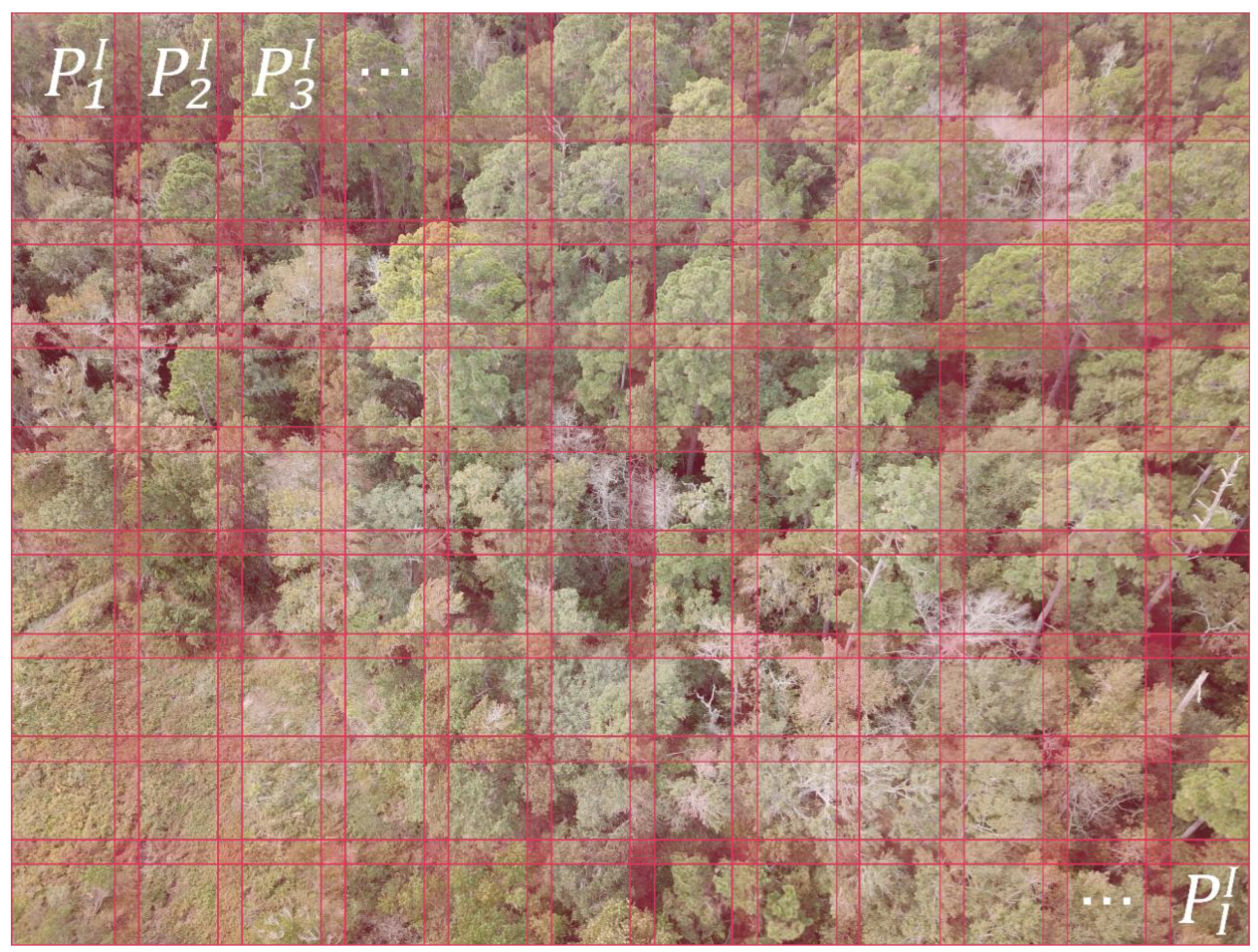
2.3.1. Model Architectures and Tiling

We trained two YOLO object detection model architectures, YOLOv4-tiny and YOLOv5n. YOLO models are in a class of single-shot detectors, which skip the region proposal network step found in the detection pipeline of two-stage detectors like R-CNN and Fast R-CNN [18]. This structural difference in the detection pipeline enables single-shot detectors to achieve relatively fast speeds compared to two-stage detectors and makes them suitable candidates for real-time detection (Figure 4).

However, YOLO models require specific input image sizes that are much smaller than our original, large-resolution parent images. Compressing parent images down to input dimensions would cause loss of pixels and diminish the details necessary to detect small objects. We circumvented this issue by dividing each original image into smaller tiles, each of which conformed to network input dimensions (Figure 5).

We selected the smallest amount of network layers and input pixel dimensions for each model family; 416 × 416 pixels for YOLOv4-tiny and 640 × 640 pixels for YOLOv5n. This translated into smaller computational demands and faster training and inference times. It also placed the average image object’s pixel dimensions above the recommended threshold of 10% of input pixel dimensions for detection [29,30]. Furthermore, training speed was greatly accelerated by using NVIDIA CUDA (Compute Unified Device Architecture) parallel computing platform, along with NVIDIA cuDNN (CUDA Deep Neural Network) GPU-accelerated Library. All training was performed on local hardware using two notebook computers (

Table 3. Hardware specifications for two laptop computers used for this study.

System	GPU	GPU Memory	CPU	RAM
Laptop 1	NVIDIA GeForce RTX 2080 Super Max Q	8 GB	Intel Core i9-10980HK @ 2.40 GHz × 16	32 GB
Laptop 2	NVIDIA GeForce RTX 3080	12 GB	AMD Ryzen 9 5900HK	32 GB

).

2.3.2. Training with YOLOv4-Tiny

Training with YOLOv4-tiny was configured using Darknet, an open-source neural network framework [44]. In addition to tiling to input dimensions of 416 × 416 pixels, Darknet also performed multiple default image preprocessing steps before training began. These included 90-degree rotation, 15% zoom, and horizontal flipping. Our combined preprocessing steps resulted in a total of 146,040 augmented images generated from the original 978 images. After approximately 35 h of training, we achieved a best mean Average Precision ([email protected]) of 95%. During model tuning, we identified that enabling the recalculation of bounding box anchors was an important parameter for better model performance due to the appearance of our targeted image objects. When experimenting with data augmentation, a vertical flip was helpful for performance, whereas other functions like image mosaicking hindered performance. We also slowly incremented batch sizes that were a multiple of subdivision sizes to manage GPU memory issues.

2.3.3. Training with YOLOv5n

Training using YOLOv5n was performed using an open-source machine learning framework, PyTorch. All the image preprocessing steps used for YOLOv4-tiny were also adopted for YOLOv5n. The one exception was image tiles conformed with YOLOv5n’s larger input size of 640 × 640 pixels. This resulted in a slightly larger input image size to image object ratio. The training was significantly more time intensive, with 300 epochs taking six days and 13 h. A larger epoch length for training might have yielded better results, but the time intensiveness of this approach proved to be a limiting factor. We achieved the best [email protected] of 78% using YOLOv5n, but we also speculated that training results could have been better had hardware capabilities not been a constraint.

2.3.4. Model Testing

A total of 103 images not used for either model training or validation were used for model testing. Image inferencing was performed using Darknet Detector for YOLOv4-tiny and Sliced Aided Hyper Inferencing (SAHI) for YOLOv5n. At the time of this study, the SAHI library did not support YOLOv4-tiny; therefore, image slicing was used. While tiling an image is a relatively straightforward approach (Figure 5), SAHI is a recently developed technique that can be integrated directly into the inference pipeline without pretraining and uses overlapping “slices” of the original images when making detections [30]. This enabled detection of fringe objects that might be split by tiles that do not overlap. SAHI logically slices a sample image $I$ into l number of $M\times N$ overlapping slices denoted by $P_1^I, P_2^I ,P_3^I ,\dots , P_l^I$. For our model, this was 416 × 416 pixel dimensions (Figure 6). The dimensions of sample image $I$ and corresponding slice, $l$, can vary on model input requirements. Upon the creation of each slice, object detection inferencing is iteratively applied. Each new slice was offset to create 20% overlap, where overlap is a customizable hyperparameter. This process facilitated detecting small RCW cavities within one slice or RCW cavities spread across multiple slices as bounding box inferences are merged via the non-maximum suppression (NMS) algorithm.

Like training, test images are inferenced at model input dimensions or overlapping slices in the case of SAHI. However, they are not physically partitioned into tiles as in training (Figure 5). Testing was performed at a confidence threshold of 0.30, with the Intersection over Union (IoU) being the calculation determining whether a detection fell below or above that designated threshold. IoU is calculated as follows:

$$\mathrm{IoU}=\frac{\mathrm{Area}\mathrm{of}\mathrm{Overlap}}{\mathrm{Area}\mathrm{of}\mathrm{Union}}$$

(1)

A relatively low confidence threshold of 0.30 was selected to intentionally include a larger number of detections, some of which were anticipated to be avoidable false positives (FP). Our rationale behind this was to preserve the occasional true positive (TP) that occurred at lower confidence intervals at the expense of filtering through a larger amount of FP. In this way, we tuned our model to our specific problem and approach, which later included semi-automated review of survey images. Model testing outcomes were summarized with TP, FP, false negatives (FN), and true negatives (TN), and then precision, recall, and F1 score metrics defined in Equations (2)–(4) were used to measure the performance of YOLOv4-tiny and YOLOv5n test results qualitatively:

$$\mathrm{precision}=\frac{\mathrm{TP}}{\mathrm{TP}+\mathrm{FP}}$$

(2)

$$\mathrm{recall}=\frac{\mathrm{TP}}{\mathrm{TP}+\mathrm{FN}}$$

(3)

$$\mathrm{F}1\mathrm{score}=\frac{2\times \left(\mathrm{Precision}\times \mathrm{Recall}\right)}{\mathrm{Precsion}+\mathrm{Recall}}$$

(4)

2.4. Surveying and Field Validation

2.4.1. Pedestrian

Pedestrian surveys were conducted in Compartments 31–33 in spring of 2022. Traditional survey methods for RCW cavity trees call for transect spacing of 91 m in very open pine stands and 46 m in areas of dense midstory [31]. We attempted to reasonably maintain this standard, although it was intermittently difficult because of very dense midstory vegetation. This standard was reasonably adhered to in foraging habitats, especially where nesting habitats occurred. Per survey protocols, areas where RCW presence could be confidently ruled out were excluded from surveys, such as riparian areas and pine stands younger than 30 years [31]. A Garmin GPSMAP 64s handheld unit was used to collect coordinate data for each new tree found. This device was accurate to within ±3 m, with a wireless protocol of 2.4 GHz @ 0 dBm nominal and battery life of up to 16 h.

2.4.2. Aerial: Manual Review and Semi-Automation

Aerial surveys were conducted in all survey Compartments in spring 2022. Image capture parameters were more regimented to ensure consistent and thorough survey coverage that mimicked established protocols. Mission planning was performed in DroneDeploy and DroneLink app services, with flights broken into approximately 18-to-30-min missions. Our total survey area of 1264 ha area was quite large for a multi-rotor UAS, so it took two pilots several flights over three weeks to cover the entire area. Additionally, battery life limitations and line-of-sight limitations further necessitated the use of small survey flights. Flight parameters used were 70–75% front overlap, 60–65% side overlap, and a horizontal flight speed of approximately 4 m per second. Altitude was 46 to 76 m, gimbal angle was 45° oblique, and terrain awareness was enabled to allow the UAS to maintain a consistent above-ground altitude (AGL). Based on these inputs, mission planning apps would create an automated flight path that the UAS followed while capturing photos at the designated survey overlap.

Total survey images collected was approximately 14,000 for Compartments 31–33. Semi-automated review was performed by inferencing survey images using the YOLOv4-tiny model and visually inspecting the subset of images containing detections afterward. With detections delimited by bounding boxes, semi-automated review proved more time efficient because a much smaller pixel area was defined by the bounding box or boxes in each image. This eliminated the error-prone and time-consuming process of manually reviewing the entire pixel area of one original image. During semi-automated review, model detections were confirmed as either FP or TP, with the latter case being added to a list of images to ground-truth later.

2.4.3. Field Validation

Following inference of survey images, ground-truthing of true-positive cavity tree detections was performed. The latitude and longitude coordinates were included within each UAS image’s metadata and extracted for field validation where images contained confirmed true positives. A Garmin GPSMAP 64 s handheld unit was used to navigate to locations and confirm a cavity tree’s presence and gather exact location coordinates. Results from pedestrian surveys and semi-automated review of YOLO model results were later compared.

3. Results

3.1. Model Testing Results

With a confidence threshold of 0.30 for 103 testing images, F1 scores of 0.85 and 0.82 were achieved using YOLOv4-tiny and YOLOv5n, respectively. Additionally, YOLOv4-tiny had an [email protected] (IoU threshold = 0.5) of 95% while YOLOv5n had an [email protected] (IoU threshold = 0.5) of 78%. Overall, YOLOv4-tiny outperformed YOLOv5n, including the amount of accurate positive predictions (TP), the amount of missed detections (FN), and precision (

Table 4. Summary of RCW cavity detection performance by YOLOv4-tiny and YOLOv5n.

Metric	YOLOv4-Tiny	YOLOv5n
TP (true positive)	130	92
FP (false positive)	37	2
FN (false negative)	8	39
TN (true negative)	-	-
precision	0.7784	0.7023
recall	0.942	0.9787
F1 score	0.8525	0.8178

). However, YOLOv5n performed better at not making predictions unnecessarily, with two false positives, while YOLOv4-tiny had 37 false positives. YOLOv4-tiny achieved an inferencing speed of 2.5 frames per second (fps). An existing study reported a speed of 0.5 fps and an overall mAP of 0.87 for detecting and classifying insects [25], and another study obtained a speed of 8.64 fps for their most accurate model in a study attempting to detect birds in real-time [24]. The former did not employ tiling or SAHI, and the latter targeted large image objects. Neither approach used an aerial image captured by UAS frameworks.

Results could be somewhat circumstantial when assessing detection performance on the test data. While YOLOv5n had 39 false negatives (FN) or missed cavity trees, it also tended to make stronger predictions in the form of more stable bounding boxes and higher confidence levels. Most cavity trees were detected by both models, while some cavity trees were uniquely found by one model (Figure 7). Collectively, both models found all the cavity trees in the testing dataset.

3.2. Comparing UAS and Pedestrian Survey Results in Compartments 31–33

The UAS-based survey and the proposed YOLO-based inference recognized true positive (TP) cavity trees in all active clusters within Compartments 31–33, except clusters 31-1 and 31-6. No detections were generated in any clusters designated as inactive or recruitment, where the latter designates clusters with pseudo-cavities installed into trees but not eventually used by RCWs. Not all images determined to be true positives (TP) during the semi-automated review were confirmed RCW cavity trees following ground-truthing. In total, 24 of 31 true positives were confirmed to contain cavity trees, with some images containing more than one cavity tree. In clusters where detections were made, not every active tree within that cluster was identified using the proposed methods, but minimally one or more detections were generated amongst a cluster’s collective trees. Pedestrian surveys found one unique discovery in cluster 31-1, whereas aerial surveys discovered five unique detections. Of those five, three were just north of cluster 33-2, a previously labeled inactive cluster and a newly updated active one because of these discoveries. The remaining two were both inactive RCW cavities but unassociated with any existing clusters. Ground crews confirmed that unique aerial survey detections were enveloped in thick, almost impenetrable vegetation. In total, aerial surveys resulted in ten newly located trees, five of which were unique detections. Traditional pedestrian methods located six new trees, one of which was a unique detection. Both methods combined located eleven new cavity trees (Figure 8).

4. Discussion

4.1. Interpretation of Results

While YOLOv5n resulted in poorer training performance than its YOLOv4-tiny counterpart, it still produced comparable testing performance or F1 scores, despite curtailed training time. Because of hardware constraints and excessively long training time, YOLOv5n was forced to stop with a small number of epochs, indicating it may have had more performance potential. Despite that, YOLOv5n still managed to generate an F1 score of 0.82, compared with YOLOv4-tiny’s F1 score of 0.85. This is compared to relatively dissimilar training metrics of 0.78 [email protected] for YOLOv5n and 0.95 [email protected] for YOLOv4-tiny. We speculate that YOLOv5n might have been a better-performing model if computational demands were not a limiting factor. Indicators, such as more appropriately placed bounding boxes around cavities, predictions at higher confidence levels, and a smaller likelihood for false positives supported this conclusion.

Semi-automation of aerial images compared with pedestrian survey methods produced mixed results, with aerial surveys being the most successful at generating unique detections of undiscovered RCW cavity trees. However, in two out of eight instances, aerial surveys did not create detections in existing and active RCW clusters. This could be partly due to overexposed images, which was an issue with groups of aerial survey images from regions of Compartment 31. It was noted during a semi-automated review that moderate-to-low exposure images were more likely to contain detections, even if they were false positives. Those exceptions aside, aerial surveys were minimally successful at creating detections within most existing clusters while also detecting five new RCW cavity trees that were not found during pedestrian surveys. Conversely, pedestrian surveys detected one new cavity tree in cluster 31-1 that aerial surveys did not, but this anomaly also occurred in the previously mentioned area of overexposed images. This could be a coincidence, although we speculate that overexposed images could have attributed to this aberration.

4.2. Implications of Results

The proposed semi-automated methods can be used to minimally locate one or more trees in most RCW clusters where vegetation is dense and obstructs visual observations. Although there were rare instances where no cavity trees were detected in a cluster, the same applied and can be said about pedestrian methods in our results. We used our model for a semi-automated review of still-image datasets, but more detections might be possible once fully automated real-time detection is achieved. Because the forest canopy is constantly obscuring and occluding cavity trees, the window of opportunity to observe cavity trees is brief, so much so that even our flight planning overlap did not ensure every cavity tree was photographed between image captures. Once a model can hypothetically infer around 30 fps, these glimpses of opportunity can be captured more effectively. While our model is currently not producing inference times capable of real-time detection, we feel we have identified the necessary model architecture and parameters to realize that goal eventually.

Despite a sizable number of false positives after inferencing survey areas with YOLOv4-tiny, we drew similar conclusions to previous work regarding semi-automated review [26]. Namely, the presence of bounding boxes tremendously improved the speed and efficiency of locating cavity trees during the review. Namely, the presence of bounding boxes tremendously improved the speed and efficiency of locating cavity trees during the review. It did so by eliminating most of the photos from consideration while also focusing reviewers’ attention on a specific delimited area rather than the entire photo. The latter method proved to be tedious, most likely error-prone [45], and difficult to perform attentively for prolonged periods. While YOLOv5n was not as effective at locating cavity trees, it produced disparately fewer false positives, making semi-automated review even less time-consuming. The generation of false positives amongst modeling techniques is of interest to researchers [6] and will be an important consideration for our future work once fully automated detection is employed. Semi-automated review provides an opportunity to filter out false positives, but fully automated detection would result in significant inefficiencies were ground-truthing performed for excessive amounts of false positives in the case of YOLOv4-tiny.

The largest hindrances to model development were a relatively small amount of data for model training and hardware limitations. Larger amounts of annotated training data and images collected where cavity trees occur in a variety of lighting, environmental, and orientational scenarios would greatly enable model development. Despite these advantages, they are counteracted by the budgetary and time constraints inherent in creating such large datasets. This was our dilemma and a limiting factor other researchers confronted, too [26]. That said, it was our goal to illustrate that small object detection could be achieved with a relatively small dataset. We felt we accomplished that goal and consequently demonstrated that the conservation goals of RCW and other potential wildlife groups can be enabled without dedicating large amounts of resources to data collection during model development.

Our semi-automated methods were also developed in such a way that they could be implemented practically. With RCWs being such an intensively managed species by a variety of agencies, the ability to perform accurate, reliable, and fast presence surveys can significantly enable management activities that cannot commence until surveys are completed per RCW Recovery Plan protocols [31]. This is particularly relevant to the US Forest Service, as they are the primary public agency responsible for managing RCW populations occurring on public lands. While RCW management protocols and objectives have not changed, the Forest Service has seen a steady decline in staff because of a paradigmatic shift towards wildfire suppression and other priorities [46,47]. This includes a 39% reduction in all non-fire personnel and a 41% increase in the annual budget towards wildland fire management by the Forest Service between 1995 and 2018 [46]. Therefore, novel and more efficient survey methods are paramount, particularly where they can assist understaffed agencies like the Forest Service to better accomplish their RCW conservation goals.

In addition to increased efficiency, our review of UAS methods provides strong evidence that disturbances to RCWs are most likely mitigated when compared with pedestrian surveys. This is especially true in areas of dense midstory, which make navigation on foot much more cumbersome. The process is often loud, disruptive, and arguably a fruitless effort in areas where thick vegetation makes observations nearly impossible from the forest floor. Furthermore, an aerial survey significantly enhances personnel safety in hazardous workplace environments, where dehydration, tripping and falling hazards, and exhaustion are common workplace hazards.

4.3. Limitations

Computational demands may become prohibitive when training computer vision models, but alternatives are available. Powerful cloud computing services, like Google Colab or Amazon SageMaker, can substitute for local computing and enable faster model training. In the field, aerial surveys using the UAS introduced several challenges, the two most significant being lighting conditions and line-of-sight obstructions. Bright lighting, combined with harsh shadows that are common in a forested landscape, greatly inhibited the ability to make successful observations of cavity trees. Uniform lighting scenarios in the early hours or during partial to full cloudy conditions made cavity detection more likely. Moreover, current FAA Part 107 Rules and Regulations limit UAS pilots to flying within line-of-sight of the aerial vehicle. While intermittent areas of development, such as roads, agricultural areas, or prairies, enabled suitable line-of-sight conditions, it was sometimes difficult to locate launch sites because our study area consisted of a tall, forested landscape.

4.4. Future Works

Future projects will focus on fine-tuning model performance while also working towards actual real-time deployment with the UAS. It may require integrating in-flight hardware with an embedded edge AI computing device such as NVIDIA TX1 or TX2 processor to deploy the model in real-time or leveraging already integrated UAS hardware. It is also possible to geospatially locate each detection with point data during real-time surveying. Conceivably, surveys would consist of UAS flights that create an array of points of interest, and then much smaller pedestrian surveys would review them.

Ensemble is one promising technique for combining the predictive powers of the two models used in this study. As mentioned, both the models included unique predictions, indicating that enabling them to cross-validate each other might lead to more comprehensive detection power. However, the computational demands are larger when employing an ensemble method and would need to be addressed before attempting its use. It is also possible to begin incorporating a classification regime into model training, where the model identifies separate phenomena that might help with monitoring efforts.

5. Conclusions

With efficient and accurate detection in wildlife monitoring being an important conservation objective, real-time detection has the potential to further refine methods already using deep learning analysis tools. In our study, two YOLO models, YOLOv4-tiny and YOLOv5n, combined with tiling and SAHI strategies demonstrated their ability to make accurate detections of RCW cavity trees, which we feel is a case study that pushes the boundaries of automating small wildlife detection in complex, high-resolution scenarios. With YOLO models being some of the fastest, state-of-the-art deep learning architectures, our model development is a strong step toward eventual real-time detection. Our results demonstrate that a semi-automated review of UAS survey images can locate RCW cavity trees and clusters more reliably than traditional pedestrian methods. These methods could immediately begin substituting for pedestrian methods in difficult environments, thereby enabling safer operations for personnel and even more accurate survey results. When real-time detection is deployed successfully, it is conceivable that cavity trees could be detected with increasingly more confidence. Most notably, our results were the product of a relatively small training sample dataset and, therefore, can be reasonably applied by wildlife managers with small-object detection problems in heterogeneous environments.

References

1. Pennekamp, F.; Schtickzelle, N. Implementing Image Analysis in Laboratory-Based Experimental Systems for Ecology and Evolution: A Hands-on Guide. Methods Ecol. Evol. 2013, 4, 483–492. [Google Scholar] [CrossRef]
2. Weinstein, B.G. A Computer Vision for Animal Ecology. J Anim. Ecol. 2018, 87, 533–545. [Google Scholar] [CrossRef] [PubMed]
3. Borowiec, M.L.; Dikow, R.B.; Frandsen, P.B.; McKeeken, A.; Valentini, G.; White, A.E. Deep Learning as a Tool for Ecology and Evolution. Methods Ecol. Evol. 2022, 13, 1640–1660. [Google Scholar] [CrossRef]
4. Seymour, A.C.; Dale, J.; Hammill, M.; Halpin, P.N.; Johnston, D.W. Automated Detection and Enumeration of Marine Wildlife Using Unmanned Aircraft Systems (UAS) and Thermal Imagery. Sci. Rep. 2017, 7, 45127. [Google Scholar] [CrossRef] [PubMed]
5. Hodgson, J.C.; Mott, R.; Baylis, S.M.; Pham, T.T.; Wotherspoon, S.; Kilpatrick, A.D.; Raja Segaran, R.; Reid, I.; Terauds, A.; Koh, L.P. Drones Count Wildlife More Accurately and Precisely than Humans. Methods Ecol. Evol. 2018, 9, 1160–1167. [Google Scholar] [CrossRef]
6. Corcoran, E.; Winsen, M.; Sudholz, A.; Hamilton, G. Automated Detection of Wildlife Using Drones: Synthesis, Opportunities and Constraints. Methods Ecol. Evol. 2021, 12, 1103–1114. [Google Scholar] [CrossRef]
7. Yi, Z.-F.; Frederick, H.; Mendoza, R.L.; Avery, R.; Goodman, L. AI Mapping Risks to Wildlife in Tanzania: Rapid Scanning Aerial iImages to Flag the Changing Frontier of Human-Wildlife Proximity. In Proceedings of the IEEE International Geoscience and Remote Sensing Symposium IGARSS, Brussels, Belgium, 11–16 July 2021; pp. 5299–5302. [Google Scholar]
8. Bogucki, R.; Cygan, M.; Khan, C.B.; Klimek, M.; Milczek, J.K.; Mucha, M. Applying Deep Learning to Right Whale Photo Identification. Conserv. Biol. 2019, 33, 676–684. [Google Scholar] [CrossRef]
9. Hong, S.-J.; Han, Y.; Kim, S.-Y.; Lee, A.-Y.; Kim, G. Application of Deep-Learning Methods to Bird Detection Using Unmanned Aerial Vehicle Imagery. Sensors 2019, 19, 1651. [Google Scholar] [CrossRef]
10. Duporge, I.; Isupova, O.; Reece, S.; Macdonald, D.W.; Wang, T. Using Very-high-resolution Satellite Imagery and Deep Learning to Detect and Count African Elephants in Heterogeneous Landscapes. Remote Sens. Ecol. Conserv. 2021, 7, 369–381. [Google Scholar] [CrossRef]
11. Miao, Z.; Gaynor, K.M.; Wang, J.; Liu, Z.; Muellerklein, O.; Norouzzadeh, M.S.; McInturff, A.; Bowie, R.C.K.; Nathan, R.; Yu, S.X.; et al. Insights and Approaches Using Deep Learning to Classify Wildlife. Sci. Rep. 2019, 9, 8137. [Google Scholar] [CrossRef] [Green Version]
12. Guirado, E.; Tabik, S.; Rivas, M.L.; Alcaraz-Segura, D.; Herrera, F. Whale Counting in Satellite and Aerial Images with Deep Learning. Sci. Rep. 2019, 9, 14259. [Google Scholar] [CrossRef]
13. Schneider, S.; Taylor, G.W.; Linquist, S.; Kremer, S.C. Past, Present and Future Approaches Using Computer Vision for Animal Re-identification from Camera Trap Data. Methods Ecol. Evol. 2019, 10, 461–470. [Google Scholar] [CrossRef]
14. Gray, P.C.; Fleishman, A.B.; Klein, D.J.; McKown, M.W.; Bézy, V.S.; Lohmann, K.J.; Johnston, D.W. A Convolutional Neural Network for Detecting Sea Turtles in Drone Imagery. Methods Ecol. Evol. 2019, 10, 345–355. [Google Scholar] [CrossRef]
15. LeCun, Y.; Bengio, Y.; Hinton, G. Deep Learning. Nature 2015, 521, 436–444. [Google Scholar] [CrossRef] [PubMed]
16. Pouyanfar, S.; Sadiq, S.; Yan, Y.; Tian, H.; Tao, Y.; Reyes, M.P.; Shyu, M.-L.; Chen, S.-C.; Iyengar, S.S. A Survey on Deep Learning: Algorithms, Techniques, and Applications. ACM Comput. Surv. 2019, 51, 92. [Google Scholar] [CrossRef]
17. Dargan, S.; Kumar, M.; Ayyagari, M.R.; Kumar, G. A Survey of Deep Learning and Its Applications: A New Paradigm to Machine Learning. Arch. Computat. Methods Eng. 2020, 27, 1071–1092. [Google Scholar] [CrossRef]
18. Redmon, J.; Divvala, S.; Girshick, R.; Farhadi, A. You Only Look Once: Unified, Real-Time Object Detection. In Proceedings of the IEEE Conference on Computer Vision and Pattern Recognition (CVPR), Las Vegas, NV, USA, 27–30 June 2016; pp. 779–788. [Google Scholar]
19. Liu, M.; Wang, X.; Zhou, A.; Fu, X.; Ma, Y.; Piao, C. UAV-YOLO: Small Object Detection on Unmanned Aerial Vehicle Perspective. Sensors 2020, 20, 2238. [Google Scholar] [CrossRef] [PubMed]
20. Wu, W.; Liu, H.; Li, L.; Long, Y.; Wang, X.; Wang, Z.; Li, J.; Chang, Y. Application of Local Fully Convolutional Neural Network Combined with YOLO v5 Algorithm in Small Target Detection of Remote Sensing Image. PLoS ONE 2021, 16, e0259283. [Google Scholar] [CrossRef] [PubMed]
21. Wang, X.; Zhao, Q.; Jiang, P.; Zheng, Y.; Yuan, L.; Yuan, P. LDS-YOLO: A Lightweight Small Object Detection Method for Dead Trees from Shelter Forest. Comput. Electron. Agric. 2022, 198, 107035. [Google Scholar] [CrossRef]
22. Linlong, W.; Huaiqing, Z.; Tingdong, Y.; Jing, Z.; Zeyu, C.; Nianfu, Z.; Yang, L.; Yuanqing, Z.; Huacong, Z. Optimized Detection Method for Siberian Crane (Grus Leucogeranus) Based on Yolov5. In Proceedings of the 11th International Conference on Information Technology in Medicine and Education (ITME), Wuyishan, China, 19–21 November 2021; pp. 1–6. [Google Scholar]
23. Alqaysi, H.; Fedorov, I.; Qureshi, F.Z.; O’Nils, M. A Temporal Boosted YOLO-Based Model for Birds Detection around Wind Farms. J. Imaging 2021, 7, 227. [Google Scholar] [CrossRef]
24. Santhosh, K.; Anupriya, K.; Hari, B.; Prabhavathy, P. Real Time Bird Detection and Recognition Using TINY YOLO and GoogLeNet. Int. J. Eng. Res. Technol. 2019, 8, 1–5. [Google Scholar]
25. Bjerge, K.; Mann, H.M.R.; Høye, T.T. Real-time Insect Tracking and Monitoring with Computer Vision and Deep Learning. Remote Sens. Ecol. Conserv. 2022, 8, 315–327. [Google Scholar] [CrossRef]
26. Andrew, M.E.; Shephard, J.M. Semi-Automated Detection of Eagle Nests: An Application of Very High-Resolution Image Data and Advanced Image Analyses to Wildlife Surveys. Remote Sens. Ecol. Conserv. 2017, 3, 66–80. [Google Scholar] [CrossRef]
27. Mishra, P.K.; Rai, A. Role of Unmanned Aerial Systems for Natural Resource Management. J. Indian Soc. Remote Sens. 2021, 49, 671–679. [Google Scholar] [CrossRef]
28. Anderson, K.; Gaston, K.J. Lightweight Unmanned Aerial Vehicles Will Revolutionize Spatial Ecology. Front. Ecol. Environ. 2013, 11, 138–146. [Google Scholar] [CrossRef]
29. Unel, F.O.; Ozkalayci, B.O.; Cigla, C. The Power of Tiling for Small Object Detection. In Proceedings of the IEEE/CVF Conference on Computer Vision and Pattern Recognition Workshops (CVPRW), Long Beach, CA, USA, 16–17 June 2019; pp. 582–591. [Google Scholar]
30. Akyon, F.C.; Onur Altinuc, S.; Temizel, A. Slicing Aided Hyper Inference and Fine-Tuning for Small Object Detection. In Proceedings of the IEEE International Conference on Image Processing (ICIP), Bordeaux, France, 16–19 October 2022; pp. 966–970. [Google Scholar]
31. U.S. Fish and Wildlife Service. Recovery Plan for the Red-Cockaded Woodpecker (Picoides borealis): Second Revision; U.S. Fish and Wildlife Service: Atlanta, GA, USA, 2003; pp. 1–296. [Google Scholar]
32. Ligon, J.D. Behavior and Breeding Biology of the Red-Cockaded Woodpecker. Auk 1970, 87, 255–278. [Google Scholar] [CrossRef]
33. Jusino, M.A.; Lindner, D.L.; Banik, M.T.; Walters, J.R. Heart Rot Hotel: Fungal Communities in Red-Cockaded Woodpecker Excavations. Fungal Ecol. 2015, 14, 33–43. [Google Scholar] [CrossRef]
34. Rudolph, C.D.; Howard, K.; Connor, R.N. Red-Cockaded Woodpeckers vs Rat Snakes: The Effectiveness of the Resin Barrier. Wilson Bull. 1990, 102, 14–22. [Google Scholar]
35. Christie, K.S.; Gilbert, S.L.; Brown, C.L.; Hatfield, M.; Hanson, L. Unmanned Aircraft Systems in Wildlife Research: Current and Future Applications of a Transformative Technology. Front. Ecol. Environ. 2016, 14, 241–251. [Google Scholar] [CrossRef]
36. Mulero-Pázmány, M.; Jenni-Eiermann, S.; Strebel, N.; Sattler, T.; Negro, J.J.; Tablado, Z. Unmanned Aircraft Systems as a New Source of Disturbance for Wildlife: A Systematic Review. PLoS ONE 2017, 12, e0178448. [Google Scholar] [CrossRef]
37. Krause, D.J.; Hinke, J.T.; Goebel, M.E.; Perryman, W.L. Drones Minimize Antarctic Predator Responses Relative to Ground Survey Methods: An Appeal for Context in Policy Advice. Front. Mar. Sci. 2021, 8, 648772. [Google Scholar] [CrossRef]
38. ESRI. World Imagery [basemap]. Scale Not Given. “World Imagery”. 9 June 2022. Available online: https://www.arcgis.com/home/item.html?id=226d23f076da478bba4589e7eae95952 (accessed on 20 December 2022).
39. Walters, J.R.; Daniels, S.J.; Carter, J.H.; Doerr, P.D. Defining Quality of Red-Cockaded Woodpecker Foraging Habitat Based on Habitat Use and Fitness. J. Wild. Manag. 2002, 66, 1064. [Google Scholar] [CrossRef]
40. Sardà-Palomera, F.; Bota, G.; Viñolo, C.; Pallarés, O.; Sazatornil, V.; Brotons, L.; Gomáriz, S.; Sardà, F. Fine-Scale Bird Monitoring from Light Unmanned Aircraft Systems: Bird Monitoring from UAS. Ibis 2012, 154, 177–183. [Google Scholar] [CrossRef]
41. Chabot, D.; Craik, S.R.; Bird, D.M. Population Census of a Large Common Tern Colony with a Small Unmanned Aircraft. PLoS ONE 2015, 10, e0122588. [Google Scholar] [CrossRef] [PubMed]
42. Fudala, K.; Bialik, R.J. The Use of Drone-Based Aerial Photogrammetry in Population Monitoring of Southern Giant Petrels in ASMA 1, King George Island, Maritime Antarctica. Glob. Ecol. Conserv. 2022, 33, e01990. [Google Scholar] [CrossRef]
43. Pfeiffer, M.B.; Blackwell, B.F.; Seamans, T.W.; Buckingham, B.N.; Hoblet, J.L.; Baumhardt, P.E.; DeVault, T.L.; Fernández-Juricic, E. Responses of Turkey Vultures to Unmanned Aircraft Systems Vary by Platform. Sci. Rep. 2021, 11, 21655. [Google Scholar] [CrossRef]
44. Open-Source Neural Networks in c. Available online: http://pjreddie.com/darknet/ (accessed on 20 December 2022).
45. Hollings, T.; Burgman, M.; van Andel, M.; Gilbert, M.; Robinson, T.; Robinson, A. How Do You Find the Green Sheep? A Critical Review of the Use of Remotely Sensed Imagery to Detect and Count Animals. Methods Ecol. Evol. 2018, 9, 881–892. [Google Scholar] [CrossRef]
46. National Association of Forest Service Retirees. Sustaining the Forest Service: Increasing Workforce Capacity to Increase the Pace and Scale of Restoration on National Forest System Lands; National Association of Forest Service Retirees: Milwaukee, WI, USA, 2019; p. 10. [Google Scholar]
47. Santo, A.R.; Coughlan, M.R.; Huber-Stearns, H.; Adams, M.D.O.; Kohler, G. Changes in Relationships between the USDA Forest Service and Small, Forest-Based Communities in the Northwest Forest Plan Area amid Declines in Agency Staffing. J. For. 2021, 119, 291–304. [Google Scholar] [CrossRef]
Figure 1. Aerial capture locations for 444 and 532 training sample photos taken at two average altitudes (46 m and 76 m), and the survey area later used for model testing. Photos were collected at both the CBC and the SHNF, with no training samples collected within the survey area in Compartments 31–33 on the SHNF. Coordinate System: NAD 1983 UTM Zone 15N. Our basemap was reprinted/adapted with permission from Ref. [38]. Maps throughout this article were created using ArcGIS® software by Esri. ArcGIS® and ArcMap™ are the intellectual property of Esri and are used herein under license. Copyright © Esri. All rights reserved. For more information about Esri® software, please visit www.esri.com.
Remotesensing 15 00883 g001
Figure 2. Differences between training sample images collected at altitudes of (a) 76 m and (b) 46 m. In addition to altitude, the lighting difference observed between the two photos is an example of how we attempted to create a diverse training sample image dataset. For our study, high-resolution images were collected at higher altitudes using the Mavic 2 Pro, and lower-resolution images were collected at lower altitudes with the Mavic Pro Platinum.
Remotesensing 15 00883 g002
Figure 3. Comparison of (a) a cavity tree image from the ground and (b) a cavity tree ariel image from 76 m altitude. The former serves as an example of what resin wells look like visually but was not captured aerially or used for the study’s training sample dataset. While the resin wells are the most noteworthy feature of image objects, some also include discernible cavity entrances and red bark scaling.
Remotesensing 15 00883 g003
Figure 4. The entire workflow of our model development, which consists of (a) image collection and management and (b) model training and survey image testing. Both YOLOv4-tiny and YOLOv5n were used for model training because of their fast detection or inference times and to allow for comparisons between the two YOLO versions. Tiling was used for both the models for training, while tiling was used for YOLOv4-tiny and SAHI for YOLOv5n for model inferencing.
Remotesensing 15 00883 g004
Figure 5. Example of the total pixel dimensions (3078 × 5472) of (a) an original aerial image, (b) the pixel dimensions (105 × 13) of RCW cavity image, (c) image object loss from normal compression, and (d) image object with tiling. Because our targeted image objects (i.e., cavity trees) were, on average, 1/3630, the size of an overall original image, cavity trees would be lost to image compression during model training. To address loss from compression, we used tiling, which partitions the original image into tiles of the model’s input size. This approach enabled preservation of minute details necessary for effective small-object detection. (e) An example of an original image compressed to YOLOv4-tiny input pixel dimensions without tiling. If tiling was not used, our image objects would be completely lost from image compression and prior to model training.
Remotesensing 15 00883 g005
Figure 6. A visualization of the SAHI process. An image with a resolution of 4000 × 3000 pixels is processed one slice at a time, iteratively from P 1 I ,   P 2 I   , P 3 I   ,   ,   P l I . The dimensions of each slice are 640 × 640 pixels—the slice dimension should match the computer vision model input dimensions for ideal performance. Each time a slice is inferenced, the next slice is offset at 20% overlap. This creates areas of an image that are re-inferenced by SAHI and allows for cavities to be detected across several tiles.
Remotesensing 15 00883 g006
Figure 7. Inference result on one image taken at 76 m altitude by (a) YOLOv4-tiny and (b) YOLOv5n. While all the cavity trees in test images were collectively detected by the models, some examples were uniquely detected by only one model. Specifically, YOLOv5n detected two cavities, while YOLOv4-tiny was not able to detect them.
Remotesensing 15 00883 g007
Figure 8. Map of the aerial and pedestrian survey results for new RCW cavity trees in Compartments 31–33 on SHNF. Aerial surveys detected five unique trees and discovered existing trees in six of eight active cluster sites. Pedestrian surveys discovered one unique tree, and both methods detected five of the same new trees. This ultimately resulted in ten new trees discovered by the UAS, six during traditional pedestrian surveys, and eleven total using both methods. Coordinate System: NAD 1983 UTM Zone 15N. Our basemap was reprinted/adapted with permission from Ref. [38]. Maps throughout this article were created using ArcGIS® software by Esri. ArcGIS® and ArcMap™ are the intellectual property of Esri and are used herein under license. Copyright © Esri. All rights reserved. For more information about Esri® software, please visit www.esri.com.
Remotesensing 15 00883 g008