Abstract
To produce highly detailed 3D models of architectural scenes, both aerial and terrestrial images are usually captured. However, due to the different viewpoints of each set of images, visual entities in cross-view images show dramatic changes. The perspective distortion makes it difficult to obtain correspondences between aerial–terrestrial image pairs. To solve this problem, a tie point matching method based on variational patch refinement is proposed. First, aero triangulation is performed on aerial images and terrestrial images, respectively; then, patches are created based on sparse point clouds. Second, the patches are optimized to be close to the surface of the object by variational patch refinement. The perspective distortion and scale difference of the terrestrial and aerial images projected onto the patches are reduced. Finally, tie points between aerial and terrestrial images can be obtained through patch-based matching. Experimental evaluations using four datasets from the ISPRS benchmark datasets and Shandong University of Science and Technology datasets reveal the satisfactory performance of the proposed method in terrestrial–aerial image matching. However, matching time is increased, because point clouds need to be generated. Occlusion in an image, such as that caused by a tree, can influence the generation of point clouds. Therefore, future research directions include the optimization of time complexity and the processing of occluded images.
1. Introduction
Image matching is at the core of the fundamental photogrammetry problem. Fast and accurate image matching is the basis of image processing. With the development of multilens cameras and the wide use of consumer-level cameras, aerial and street-level images have become the major data source for city-scale urban reconstruction. The observation angle of a single aerial or terrestrial image is limited, so the information obtained is not comprehensive. Therefore, a model reconstructed from terrestrial images usually has fine texture and almost no deformation. This model type lacks roof information, and cavities often appear at the tops of buildings. In contrast, a model reconstructed from aerial images usually has a relatively complete structure but lacks details, and the bottoms of the buildings are prone to blurring.
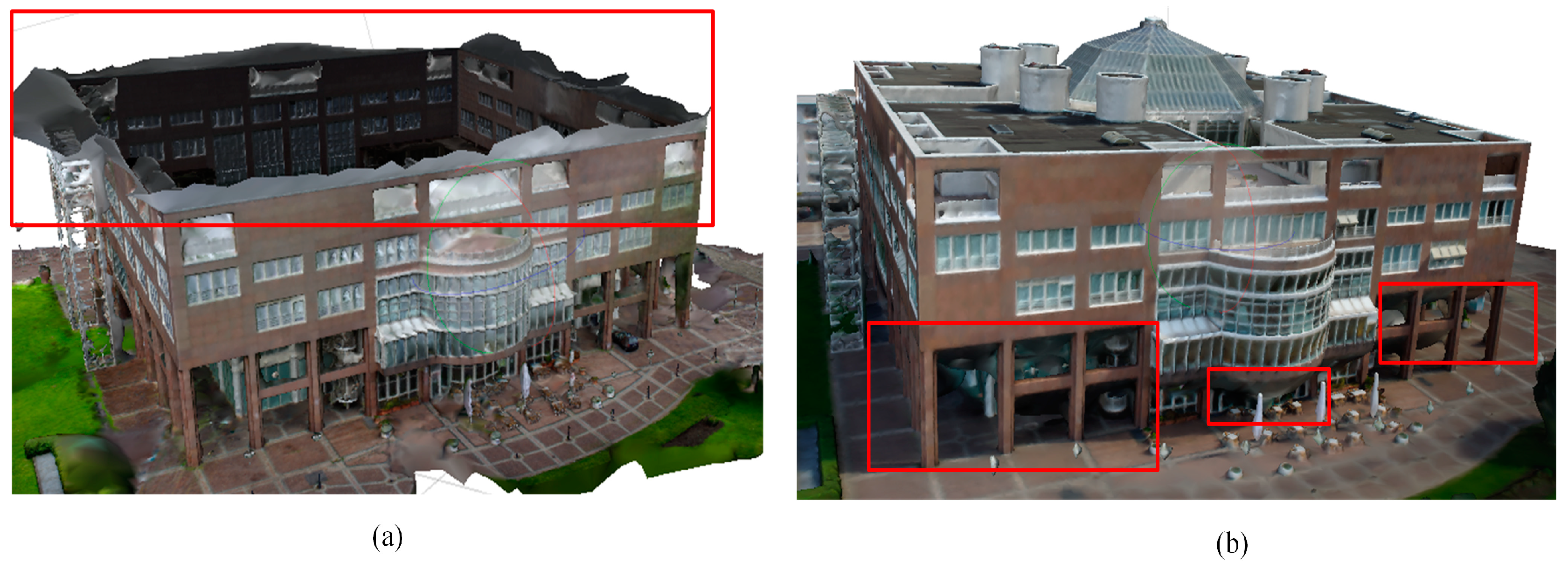
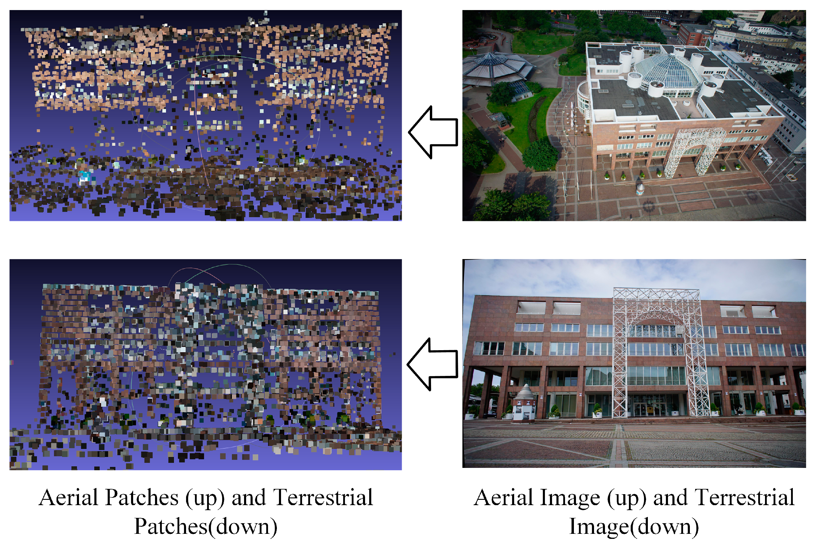
Recent studies [1,2,3] have demonstrated that a combination of terrestrial and aerial images is an effective way to improve the accuracy of 3D reconstructions. Figure 1 shows models that were reconstructed from aerial and terrestrial images. The ground model (built by terrestrial images) is highly detailed but lacks roof information; in contrast, an aerial model (built by aerial images) is more complete but less detailed, especially at the bottom parts of the buildings [1].

Figure 1.
Reconstructed models from images collected from different perspectives. (a) The ground model. (b) The aerial mode.
The combination of terrestrial–aerial photogrammetry for 3D reconstruction has been used in cultural heritage conservation [4,5], archaeological excavations [6], landslide reconstruction [7], and urban environmental studies [8].
Image alignment is necessary to integrate multisource images. However, in multi-source image acquisition, differences in resolution, viewpoint, scale, sensor models, and illumination conditions will lead to feature confusion and object occlusion problems in the images [9]. For aerial–terrestrial image pairs, region-based methods encounter challenges because of the drastic viewpoint change and scale change, and the performance of region-based methods decreases dramatically with the increasing geometric difference between aerial and terrestrial images [10]. Naturally, the most frequently used method for aligning aerial and terrestrial imagery is to match the images’ local features such as the scale-invariant feature transform (SIFT) [11], speeded up robust features (SURF) [12], and affine-sift (ASIFT) [13]. However, such methods cannot manage the dramatic viewpoint and scale differences between terrestrial and aerial images, and the performance of these methods degrades considerably when the translation tilt exceeds 25° [14]. The major obstacles to establishing correspondence between terrestrial-view and aerial-view images are the drastic viewpoint and scale difference. The perspective deformations caused by the drastic viewpoint and scale changes between aerial–terrestrial images severely hinder local feature extraction and matching. Occlusion and repetitive patterns common in urban scenarios also complicate this problem [15]. Discriminative feature points and robust descriptions improve the efficiency and accuracy of subsequent matching. To obtain more robust features, some researchers have proposed alleviating the difference in viewpoints by transforming images, whereas others have attempted to introduce deep-learning-based frameworks to extract image features and establish correspondences. Some researchers have pioneered different studies and discussions. Existing studies have mostly used the matching of UAV’s look-down images with reference images, whereas studies on the matching of large-inclination and multiview UAV images with reference images are relatively rare [9].
- (1)
- Image rectification-based methods. Warping all of the images to the same reference plane is a valid solution to eliminate the global geometric deformation between images [10]. Some researchers have proposed alleviating the difference in view angle by transforming images of arbitrary views into a standard view [1,16,17,18]. Maria et al. [16] transformed an arbitrary perspective view of a planar façade into a frontal view by applying an orthorectification preprocessing step. Finding a common reference plane and then projecting the images onto it is an effective method to alleviate geometric deformations [19,20,21]. However, it is not always possible to find a suitable reference plane. Thus, view-dependent rectifications that reduce the geometric distortion by correcting each pair of images individually have been proposed [10]. In the work of [22], a ground-based multiview stereo was used to produce a depth map of terrestrial images and warp the images to aerial views. Gao et al. [3] rendered 3D data onto a target view. These methods require dense reconstruction to generate the model, and the quality of the mesh model influences the synthetic image. As the quality of the synthesized images decreases, the matching performance becomes limited. Although these methods effectively reduce the variance in descriptors, the large number of matches and the ambiguous repeating structures hinder the approach [23]; it is usually acceptable for local windows rather than a whole image.
- (2)
- Deep-learning-based methods. Different from traditional methods, convolutional neural networks (CNN) extract image features; the more adaptive and robust feature descriptors are extracted through iterative learning of the neural networks. Some researchers [24,25] have obtained image feature detectors that perform better than traditional feature detectors such as SIFT. In recent years, with the development of artificial intelligence, deep-learning-based methods, such as deep feature matching (DFM) [26], SuperPoint [27], and SuperGlue [28], have also made great progress in cross-view image matching. SuperGlue [28] takes the features and the descriptors detected by SuperPoint [27] as inputs and then uses a graphical neural network to find the cross- and self-attention between features. It can significantly improve the matching performance of extracted features. However, the authors in [29] showed that due to the tradeoff between invariance and discrimination, it is generally impossible to make the network more rotation and illumination invariant. DFM [26] adopts a pretrained VGG-19 [30] extractor that is applied to the features in the terminal layers first and hierarchically matches features up to the first layers. However, DFM requires the target object to be planar or approximately planar. It should be noted that deep-learning methods cannot completely replace the classical method, and [31] proves that classical solutions may still outperform the perceived state-of-the-art approaches with proper settings.
To solve the problem of perspective distortion and scale difference, the proposed method transfers image matching into patch matching based on point clouds. The perspective distortion is reduced by projecting a local window onto a rectified patch. Different from other image rectification methods, in this paper, each extracted feature point is rectified separately. Additionally, the geometric features inherited from the point cloud can be used as geometrical constraints to remove outliers.
This can provide a basis for the integration of aerial and terrestrial images. Accurate image alignment is a prerequisite for subsequent image-processing flow, typically 3D reconstruction. The main contributions of this paper are summarized as follows:
- (1)
- A robust aerial-terrestrial image-matching method is proposed. The proposed method can address drastic viewpoint changes, scale differences, and illumination differences in the image pairs.
- (2)
- Mismatches caused by weak texture and repeated texture are alleviated. The geometric constraints between patches (inherited from the point clouds) can eliminate outliers in matching.
- (3)
- The effect of matching is not affected by the shape of the target building. The proposed method does not require the matching object to be a plane.
The rest of this paper is structured as follows. Section 2 introduces the proposed method in detail. Section 3 introduces the experimental dataset, and the performance of the proposed method is evaluated using different terrestrial–aerial images in this section. Concluding remarks are given in Section 4.
2. Materials and Methods
2.1. Overview of the Proposed Method
As aerial images and terrestrial images are captured by different platforms, the intersection angle usually exceeds 60°. The perspective distortion and scale difference caused by the drastic viewpoint change make it difficult to register the images. This study attempts to overcome this problem by establishing the closest patch to the local tangent plane of the object.
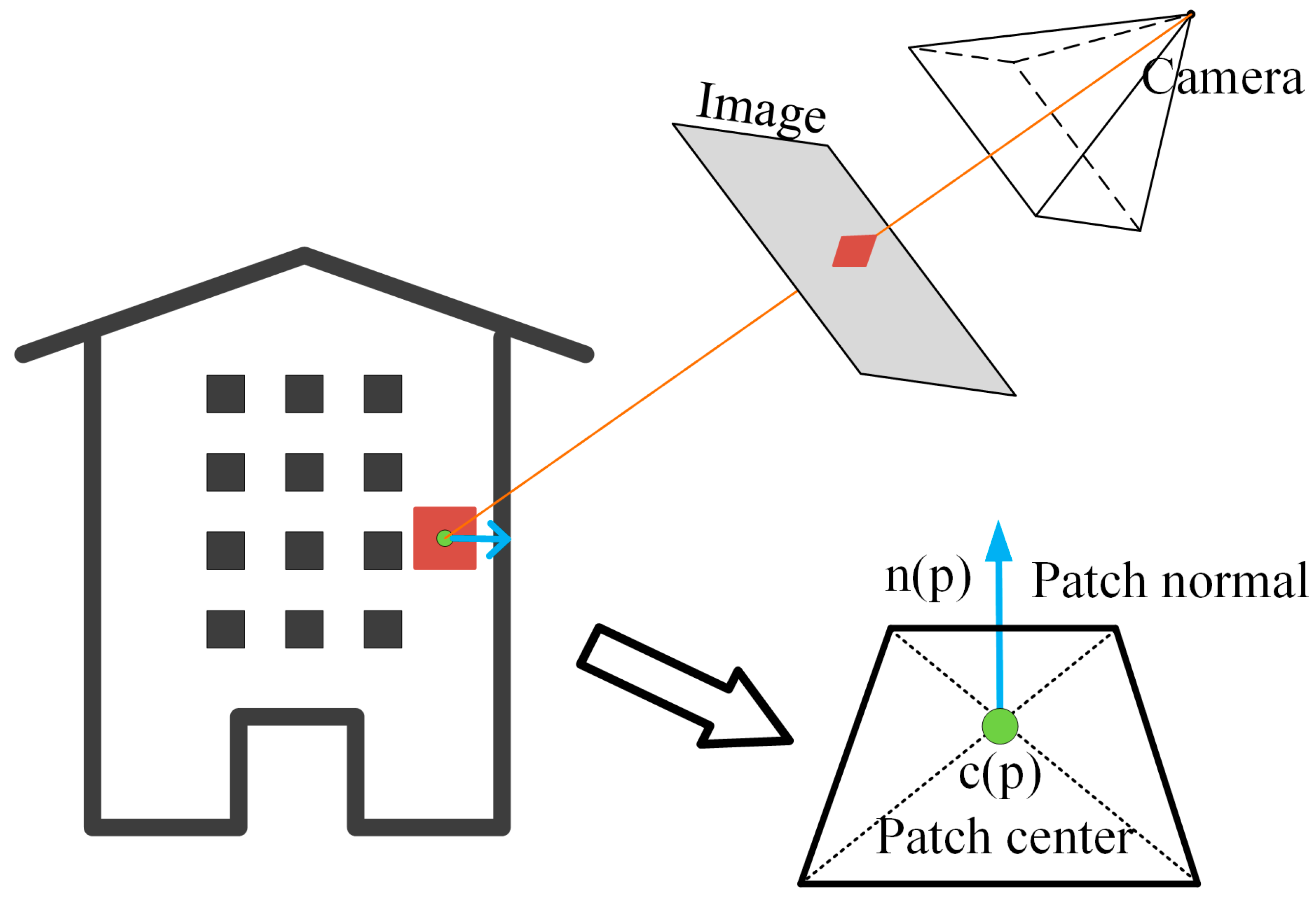
Aerial and terrestrial image alignment is performed in the following manner. First, the sparse 3D point clouds of the aerial and terrestrial images are obtained from off-the-shelf SFM (OpenMVG) [32] solutions, respectively. Because the perspective distortion of images captured by the same platform is small, feature matching between images can obtain a reliable result. The patches are built based on the point clouds and optimized to be close to the tangent plane of the object surface by the following variational patch refinement method. The perspective distortion and scale difference can be reduced when the local window of the image is projected onto the patch. The patch consists of a normal vector n(p) and a centroid c(p), as shown in Figure 2.
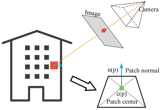
Figure 2.
Definition of a patch.
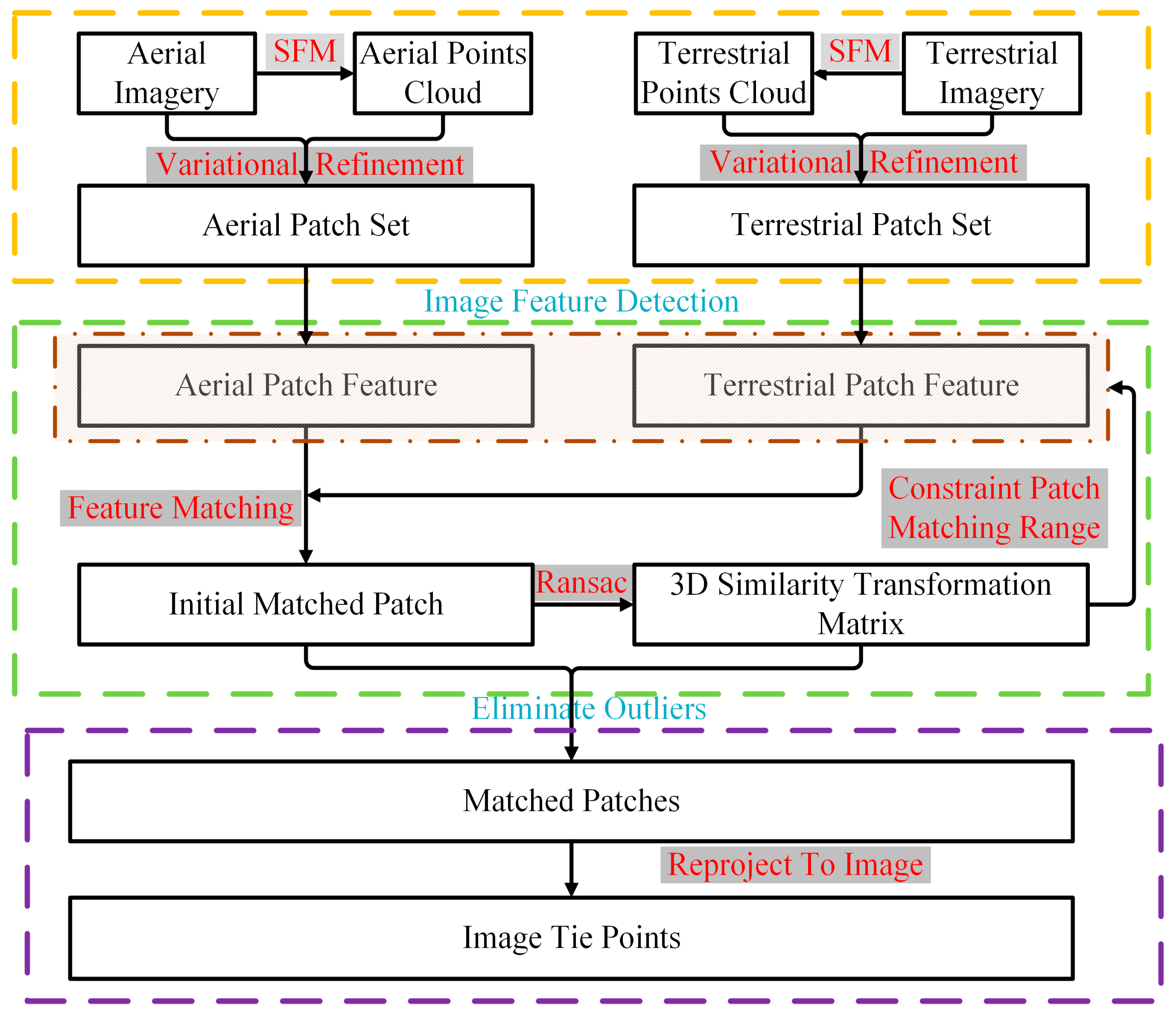
Through variational patch refinement, the features of the optimized patches can be detected from the textures projected by the images. After that, the matched patches can be obtained through feature matching. The 3D similarity transformation model estimated from the initial matched patches can be used as the geometric constraint to limit the matching range for each patch and remove outliers. The image tie points are the reprojections of matched patches. The overall workflow of the proposed approach is shown in Figure 3.
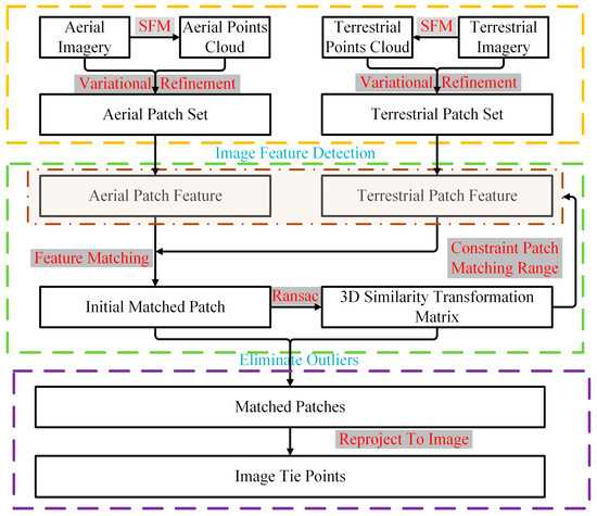
Figure 3.
Flowchart of the patch-based matching strategy.
2.2. Variational Patch Refinement
In this paper, the patch acts as a proxy for images. A pair of images are denoted as and , and a patch is denoted as T (a, b, c, D). The perspective distortion of the image can be reduced by projecting it onto the optimized patch. The aim of patch refinement is to make the position and attitude of the patch close to the surface of the object. In the optimization process, the photo-consistency is the patch refinement metric, and the normalized cross correlation (NCC) is the most common metric function. The backprojection of the patch onto images and is related to the position and attitude of the patch. The homographic transformation matrix between one image pair can be obtained. It can be denoted as H. The variational patch refinement computes the optimal patch’s position and attitude (α, β, D) iteratively, which maximizes the NCC of images.
2.2.1. Energy Function Construction
The aim of refinement is to make the patch close to the surface of the object. In this process, the photo-consistency of aerial and terrestrial images projected onto the patch is the measurement. The more similar the projection of aerial and terrestrial images is, the closer the position of the patch to the object surface. The equation for minimizing their projection similarity is formulated as follows:
where is the reprojection of image in view via patch T, and measures the similarity of the patch projection area for image pair and . is a decreasing function of a photo-consistency measure between images and at point of image ; that is, , which is opposite to the normalized cross correlation.
Then, the sum of all image pairs is minimized. The difference between and is due to the positional change in patch T. Let the normal vector of the patch be (a, b, c), and the patch plane can be expressed as:
2.2.2. Derivative of the Energy Function
To minimize the image similarity , the derivative of is taken with respect to the three parameters (α, β, D) of patch T. The derivative of the metric function with respect to T can be formulated as the product of these terms:
where H is the homographic matrix between image and image ; H’ is the normalization of H; and are the corresponding points of images and .
- Derivative of photo-consistency
The computation of the gradient that registers an image to image can be expressed as , where . The gradient is computed by applying the derivative to the pixel intensity of image .
where and are the average pixel intensities of images and , respectively. and are the standard deviations of images and , respectively. The derivative of the image intensity to the point coordinates can be represented as the image gradient of the corresponding image point in view , which can be expressed as .
- 2.
- Derivative of the homographic matrix
The homographic matrix H between two images can be expressed in terms of the projection matrix , , and patch . and are the projection matrices of images and , respectively, and patch can be expressed as .
where is the Mth row of the projection matrix .
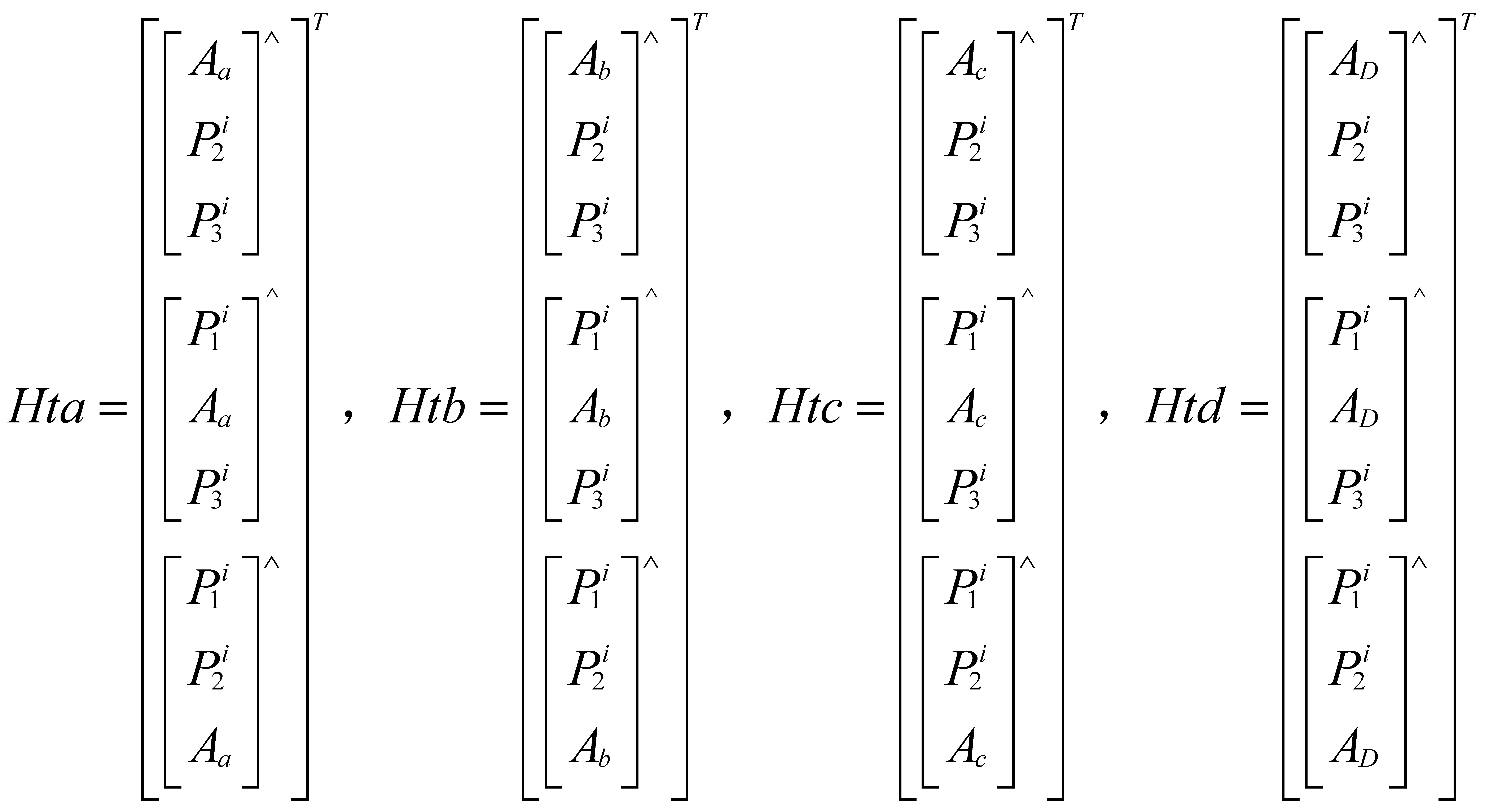
Assume that and are the corresponding points of images and . is the transformation matrix that transforms the image point to the object point on the patch. is the matrix that contains the four variables: , , , and D. Therefore, can be expressed as:
where Hta, Htb, Htc, and Htd are the coefficients of variables a, b, c, and D, respectively, separated from Ht.
Therefore:
Through the above theoretical deduction, the homographic matrix H, which contains the four variables (a, b, c, and D), can be obtained. However, the image point obtained by the homographic matrix must be homogenized. The homogeneous term is different for different image points. For the image point , the homogeneous term of its corresponding point can be obtained by multiplying the third row of H by . To obtain the derivative of the homographic matrix H, the matrix is divided by γ, so that the image point obtained by the homographic matrix is homogeneous.
where ha, hb, hc, and hD are the coefficients of the variables a, b, c, and D separated from .
Furthermore, the partial derivative of the H matrix with respect to α, β, and D can be obtained.
where:
Then, the position and normality of the patch are optimized by minimizing the metric function E(T) with respect to α, β, and D. The initial patch parameters are determined by the position of the point cloud, and its normal vector is parallel to the average optical axis of all attended images and toward the images. Then, gradient descent is used to decrease the metric function E(T) to obtain the optimal parameters.
2.2.3. Initial Parameters of the Patch
The initial patch parameters are determined by the position of the point cloud, and the centroid of patch c(p) (x, y, z) is the coordinate of each point cloud.
The normal vector n(p) is parallel to the average optical axis of all reference images and toward the images, and the equation is written as:
where is a ray formed by the patch and optical center of each reference image, and R(p) is the reference image set.
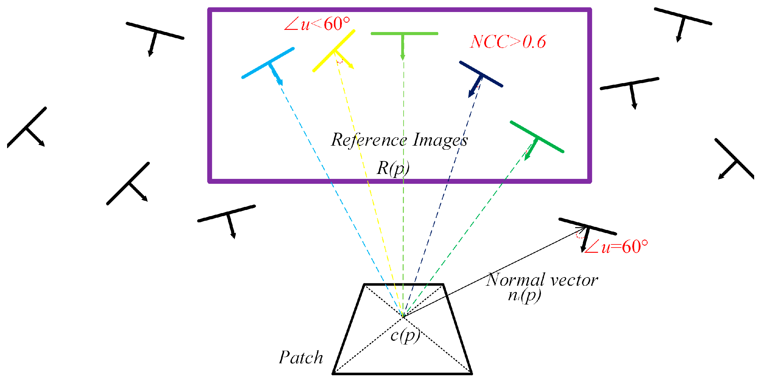
Due to the occlusion and the drastic change in the viewpoint, not all images can be used to optimize the patch, and the reference image set R(p) is selected according to the NCC threshold between the visible images and the intersection angle threshold between the images and the patches, as shown in Figure 4. The equation is written as:
where is the image that can observe the patch. is the set of reference images. is the camera optical center of the image. is the texture that image projects onto the patch. In this paper, u is set as 60°, and the threshold is set as 0.6.
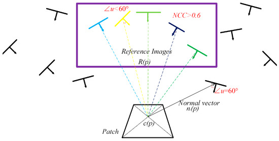
Figure 4.
Selection of reference images.
2.3. Feature Matching with the Optimized Patch
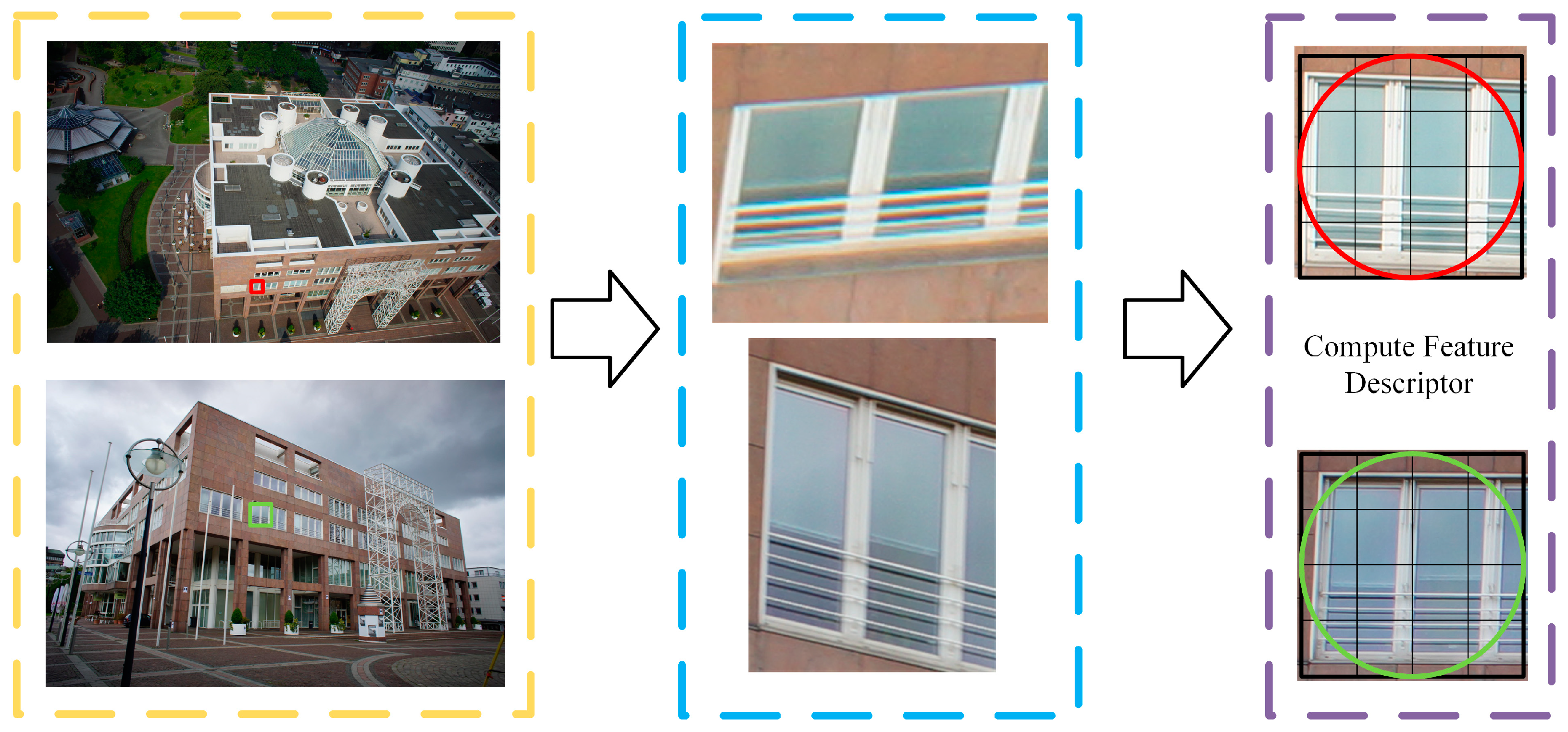
Variational patch refinement can eliminate the patch perspective distortion caused by the drastic viewpoint of the image. Figure 5 shows the effect of patch optimization. The perspective distortion and the scale difference can be eliminated. The centroid of the optimized patch represents a feature point, and the SIFT descriptor is used for matching.

Figure 5.
The effect of patch optimization. The yellow area shows the original images, the blue area shows the reprojections of the patches on the original images, and the purple area shows the rectified images on the patches.
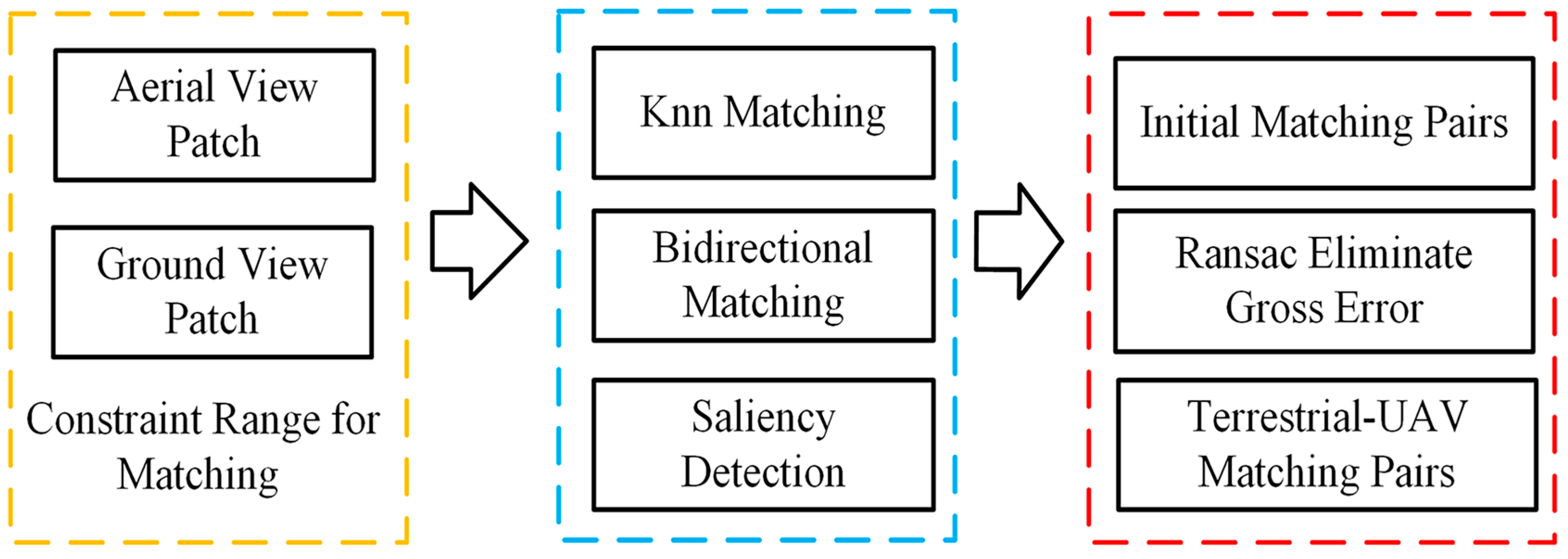
The flowchart of matching the aerial and terrestrial patches based on patch features is shown in Figure 6. First, the fast library for approximate neighbors (FLANN) is used for initial matching, and then the outliers are eliminated through cross-checking (bidirectional matching) and saliency detection using the nearest neighbor distance ratio (NNDR) test [33]. After that, the 3D spatial similarity transformation matrix between two sets of patches can be computed by RANSAC, which can be used to further remove the outliers. Furthermore, the 3D spatial similarity transformation matrix can be used as an additional geometry constraint prior to limiting the matching range of the patches, and the effect is shown in Section 3.3.1.
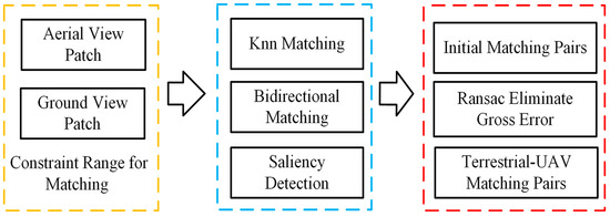
Figure 6.
Flowchart of terrestrial–aerial image matching.
3. Experiments and Analyses
In this section, an experiment is constructed to evaluate the performance of the proposed method on the ISPRS and Shandong University of Science and Technology datasets, and the proposed method is compared with two traditional and two deep-learning-based image-matching algorithms. The datasets are first described, and then the results of different datasets are evaluated.
3.1. Introduction to the Experimental Dataset
Four datasets (see Table 1) are used to evaluate the performance of the proposed method: the datasets include the ISPRS benchmark datasets collected at the Center of Dortmund and ZECHE of Zurich and the Shandong University of Science and Technology (SDUST) datasets collected at the hospital (HOSP) and academic buildings (AB). All the aerial images with position and orientation system (POS) data were captured by UAVs, but a part of the terrestrial image dataset lacks POS data.

Table 1.
Description of the four datasets used for evaluation.
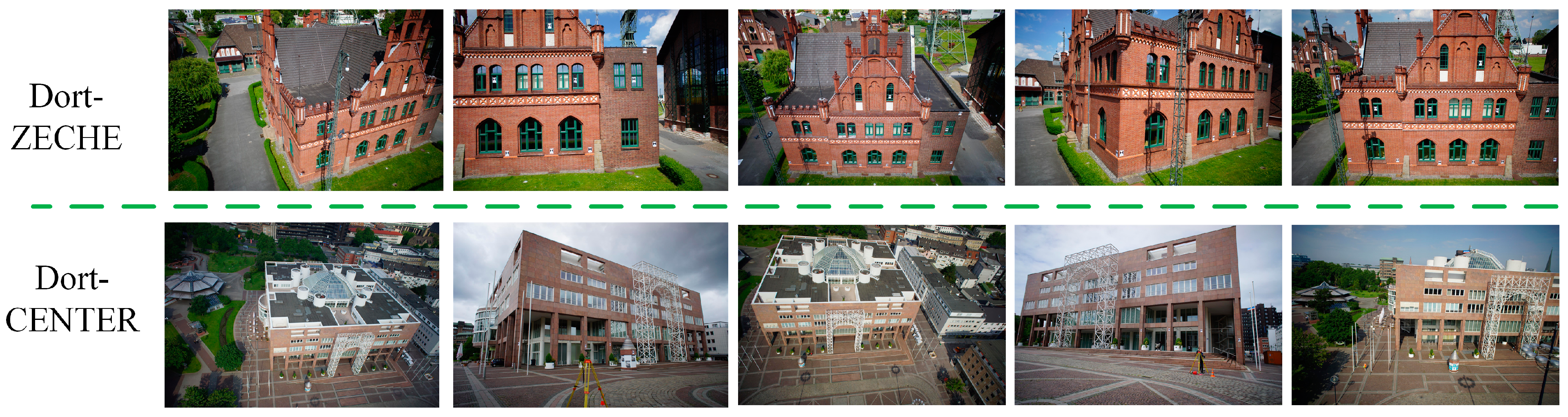
The aerial images and terrestrial images in the Center and ZECHE datasets were collected by the International Society for Photogrammetry and Remote Sensing (ISPRS) and European SDR [2] in Dortmund and Zurich, respectively, as shown in Figure 7. The aerial and terrestrial images were captured using the same sensor. The ground sample distance (GSD) of the aerial and terrestrial images ranged from 1 cm to 3 cm. A detailed description of this dataset can be found in [2].
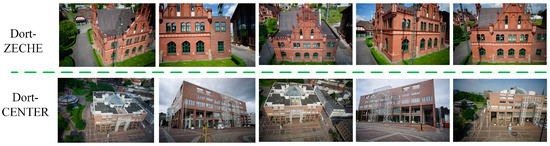
Figure 7.
Partial images of the Dort-ZECHE and Dort-CENTER datasets.
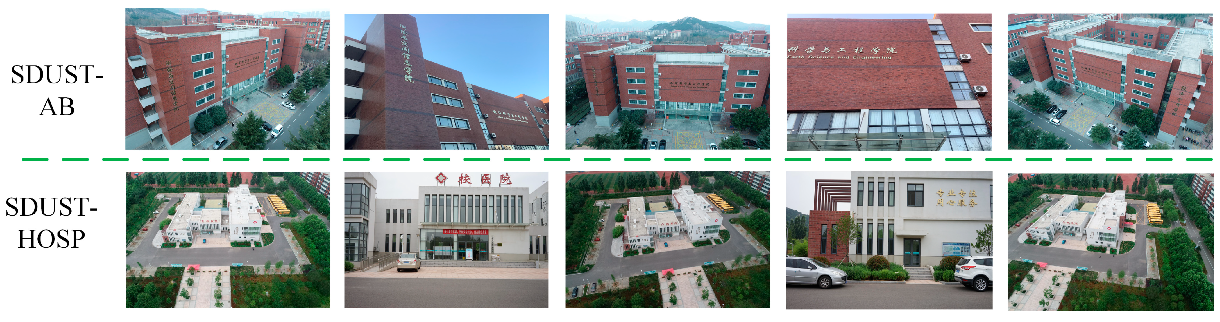
The other two datasets were collected on the campus of Shandong University of Science and Technology and include images of a hospital building and an academic building, as shown in Figure 8. Different from the ISPRS datasets, their aerial and terrestrial images were captured by different sensors, and the POS data of the ground camera are unattainable.

Figure 8.
Partial images of the SDUST-AB and SDUST-HOSP datasets.
3.2. Result of Variational Patch Refinement
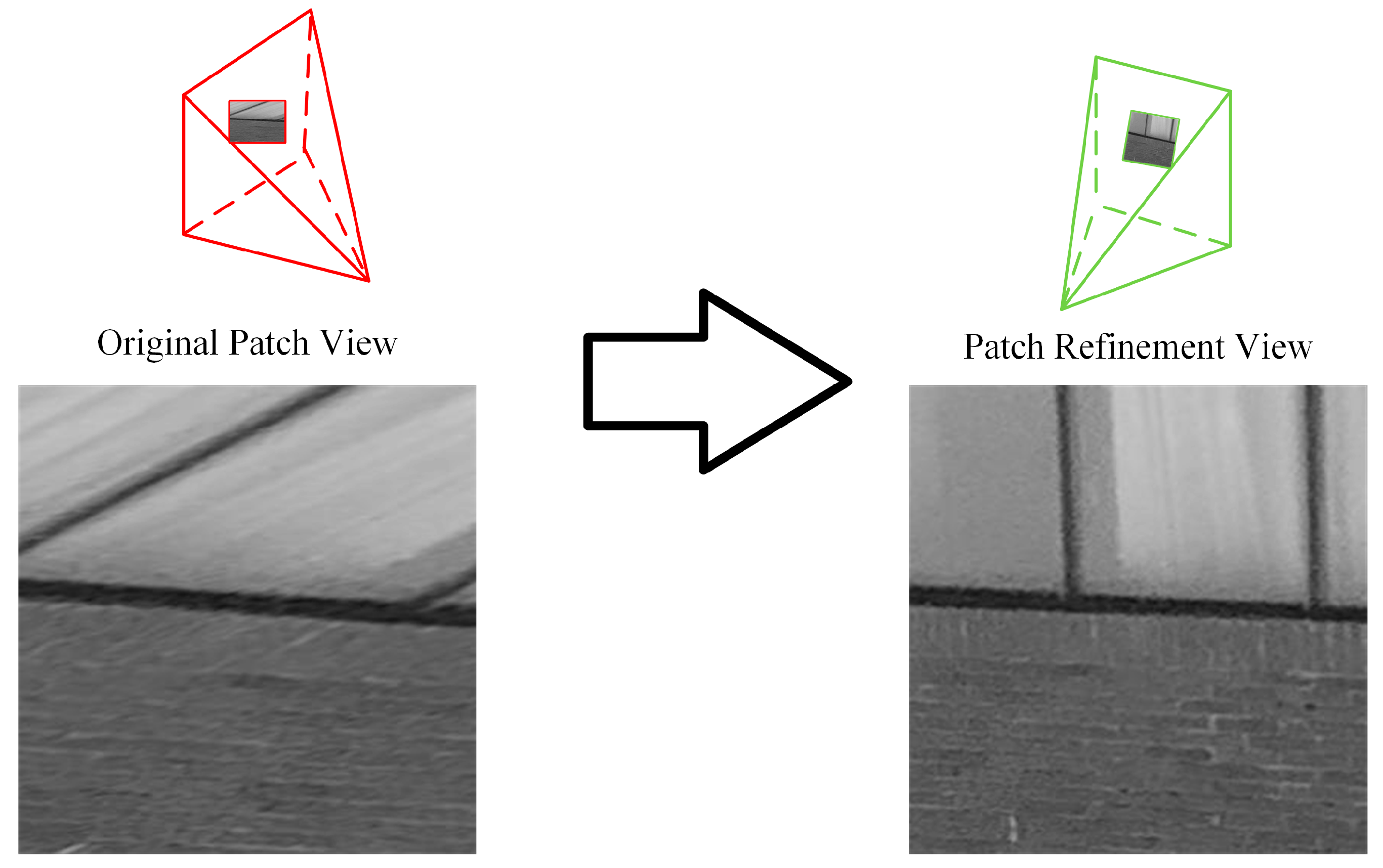
As shown in Figure 9, through variational patch refinement, the patches are optimized so that they are close to the surface of the object. Figure 10 demonstrates the effect of variational patch refinement. Note that the final image given the patch texture may change due to the optimization of the patch attitude angle. The final image with the minimal angle between its optical axis and the normal vector of the patch can be described as:
where is the normal vector of the patch, and is the principal optical axis of image .

Figure 9.
Results of variational patch refinement.

Figure 10.
Rectified effect of the refined patch. The red view frustums are original camera poses. Green view frustums are the patch refinement view.
3.3. Evaluation of the Effectiveness of the Feature-Matching Algorithms
In this section, an experiment is constructed to evaluate the performance of the proposed method on the ISPRS and Shandong University of Science and Technology datasets, and the proposed method is compared with two traditional and two deep-learning-based image matching algorithms. The evaluation results of the experiment are measured by the mean number of inliers (MNI) and mean matching accuracy (MMA, the inliers of the dataset/total matches of dataset). MMA is an important evaluation index of the image-matching algorithm, and a low accuracy means that there are many mismatches in the matching result, which will affect the subsequent tasks of image processing. However, MMA cannot fully reflect the effect of the matching algorithm. The aim of image matching is to align aerial and terrestrial images, which requires a large number of correct tie points, and the MNI can visually show whether a pair of aerial–terrestrial images can be aligned.
3.3.1. Effective Constraint Range of Feature Matching
For urban buildings, repeated façade elements are one of the feature-matching obstacles. The highly similar textures will cause more outliers in the putative matches. Sometimes the inlier matching similarity is lower than that of outliers due to highly similar textures accompanied by perspective distortion and different lighting conditions.
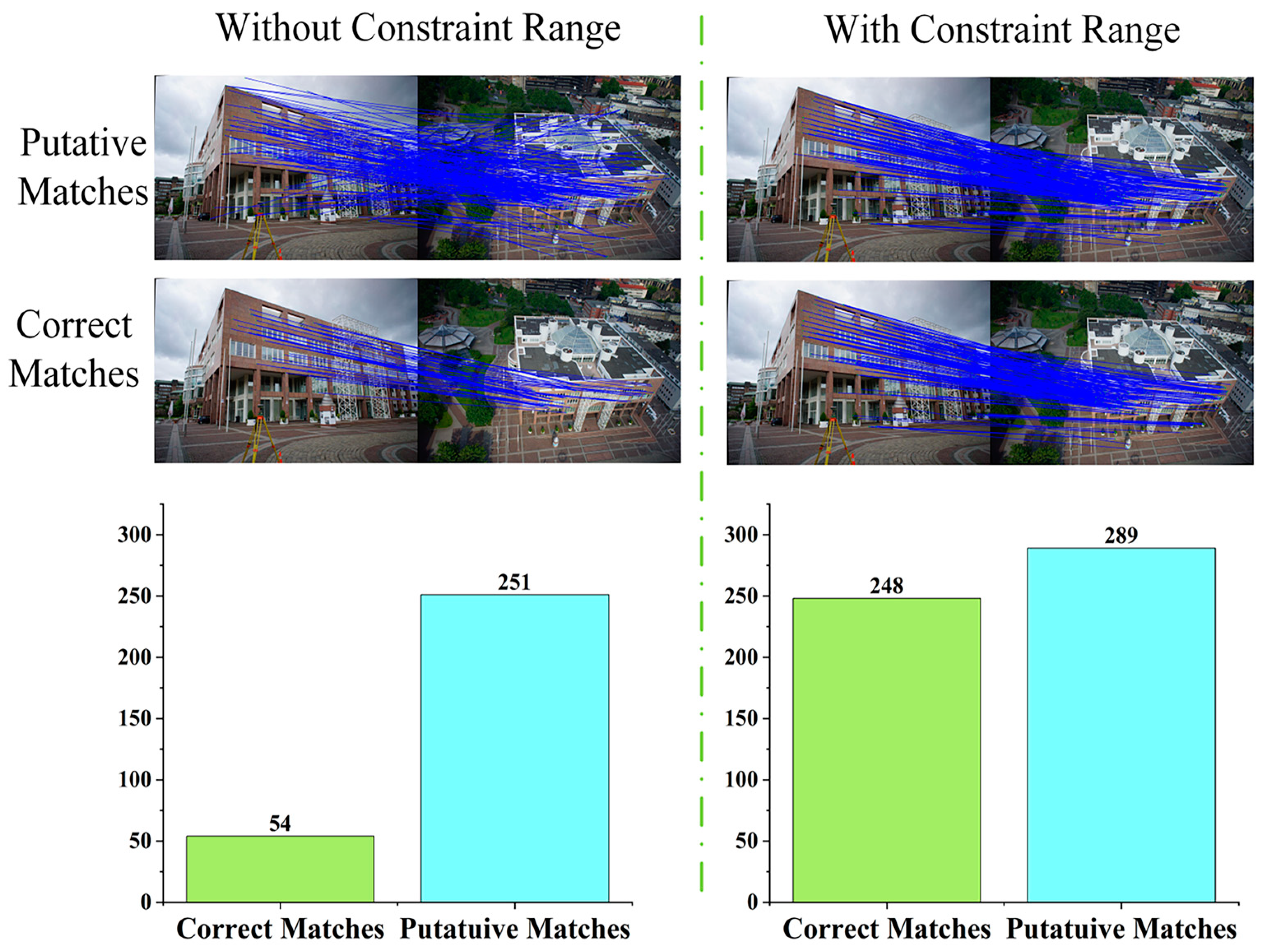
Thus, after initial feature matching, the computed 3D similar transformation can be used as the geometry constraint in patch matching. It constrains the matching range for each patch. As shown in Figure 11, feature matching without a constraint range involves 251 putative matches, and 54 are retained after eliminating the outliers; the feature matching with a constraint range involves 289 putative matches, and 248 are retained after eliminating the outliers.

Figure 11.
Feature matching constraint range results.
3.3.2. Matching Results of Public and Local Datasets
In this section, the proposed method for feature matching on these datasets is compared with the existing algorithms. Five image pairs with drastic viewpoint or scale changes are selected from each dataset for quantitative evaluation.
The results of the proposed method are compared with the result of two traditional algorithms, ASIFT [13] and GMS [34], and two deep-learning algorithms, DFM [26] and SuperGlue [28]. To be fair, the maximum number of detected feature points is limited to 4000, which is close to the number of patches corresponding to each image; the input images are resized to be the same size. For the SuperGlue method, the GitHub repository [35] with the outdoor model trained on mega depth data is used in the experiment. For DFM, the original implementation of the algorithm [36] is used in the experiment, and the radio test thresholds remain the same as the recommended settings (0.9, 0.9, 0.9, 0.9, 0.95); through testing, it is found that there may be a number of feature point limitations, and threshold changes have little impact on the number of inliers and the matching accuracy.
In image pairs 1–5, which are selected from ZECHE of the Dortmund dataset, the change in the viewing angle is drastic. The quantitative results are listed in Table 2, and a representative result is shown in Figure 12. The inlier matches are checked by the reprojection of SFM or through manually methods.
Table 2.
Quantitative results of the different methods on dataset Dort-ZECHE.
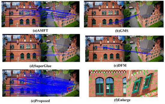
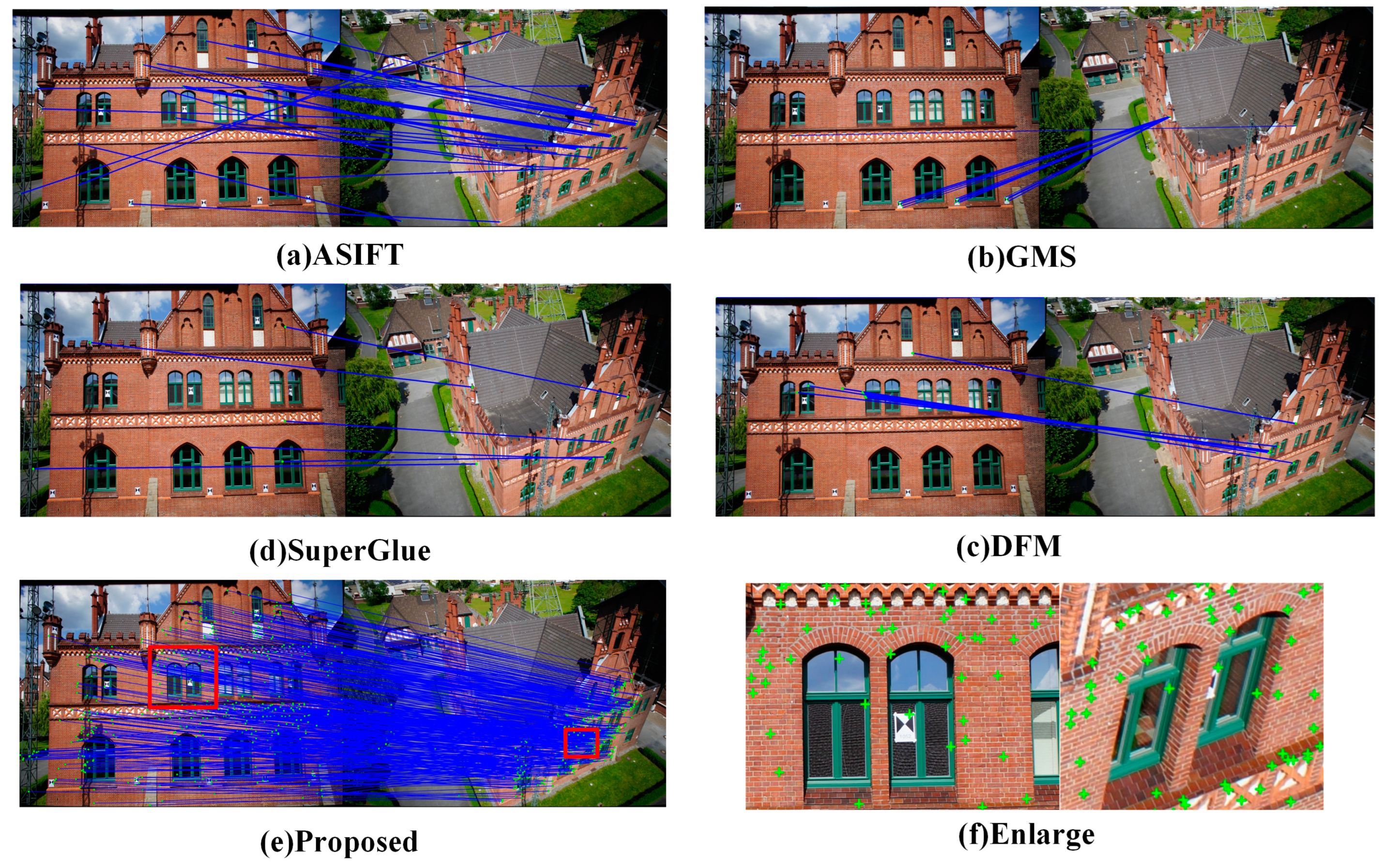
Figure 12.
Image feature-matching comparison on the ZECHE ZOLLERN (Dortmund) dataset. (a–e) show the matching results of the ASIFT, GMS, DFM, and SuperGlue algorithms, respectively. (e) shows the matching result of the proposed algorithm, and (f) shows a magnified view of the matched feature points.
A more challenging image pair, as a representative of image pairs 6–10, which were selected from Dort-Center, is shown in Figure 13. Compared with image-matching pairs 1–5, the attitude of the image pairs changes by nearly 90°, and the scale difference is more obvious. Furthermore, the lighting conditions are different because of the different capture times. As shown in Table 3, with the extreme view angle and scale difference, ASIFT and GMS almost completely fail. The method based on deep learning can only obtain a certain number of matches in this case, SuperGlue performs better than DFM, and MMA and MNI do not perform as well as the proposed algorithm.
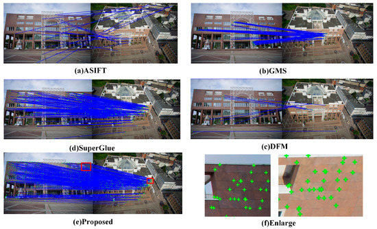
Figure 13.
Image feature-matching comparison on the Dortmund (Center) dataset. (a–e) show the matching results of the ASIFT, GMS, DFM, and SuperGlue algorithms, respectively. (e) shows the matching result of the proposed algorithm, and (f) shows a magnified view of the matched feature points.
Table 3.
Quantitative results of the different methods on dataset Dort-CENTER.
Compared with the ISPRS dataset, the SDUST dataset is more challenging in terms of evaluating the stability of the matching algorithms. Image pairs 11–15 are selected from SDUST-AB. The aerial images were captured on cloudy days, but the terrestrial images were captured on sunny days with IPAD Air-3. In particular, note that the terrestrial images only have GPS data and lack camera attitude data. The accuracy of the GPS data is low due to the capture platform. Because of the different capture equipment and weather conditions, there are significant radiometric differences in the terrestrial and aerial images, which makes image matching challenging. The matching results of the different methods are listed in Table 4, and a representative matching result is shown in Figure 14.
Table 4.
Quantitative results of the different methods on dataset SDUST-AB.

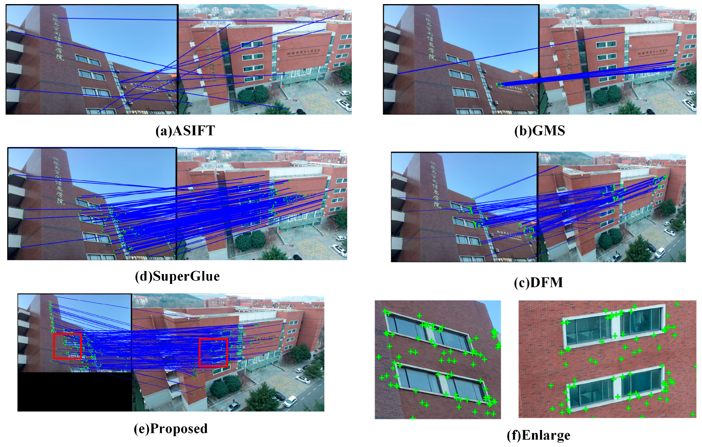
Figure 14.
Image feature-matching comparison on the Shandong University of Science and Technology dataset. (a–e) show the matching results of the ASIFT, GMS, DFM, and SuperGlue algorithms, respectively. (e) shows the matching result of the proposed algorithm, and (f) shows a magnified view of the matched feature points.
Image pairs 16–20, which are selected from SDUST-HOSP, include aerial–terrestrial images with extreme changes in scale and viewpoint. As shown in Figure 15, the scale differences between the terrestrial–aerial images are more obvious than those of the Dortmund dataset’s image pairs. In addition, the terrestrial images lack POS data.
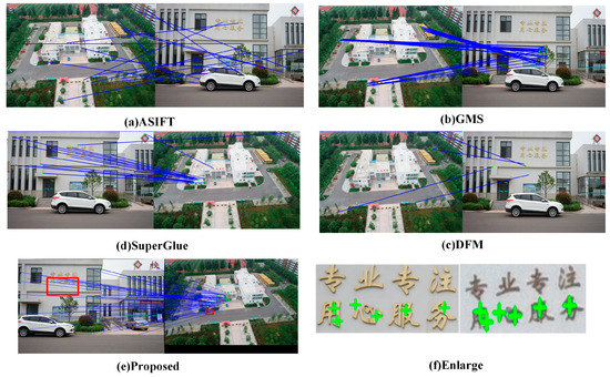
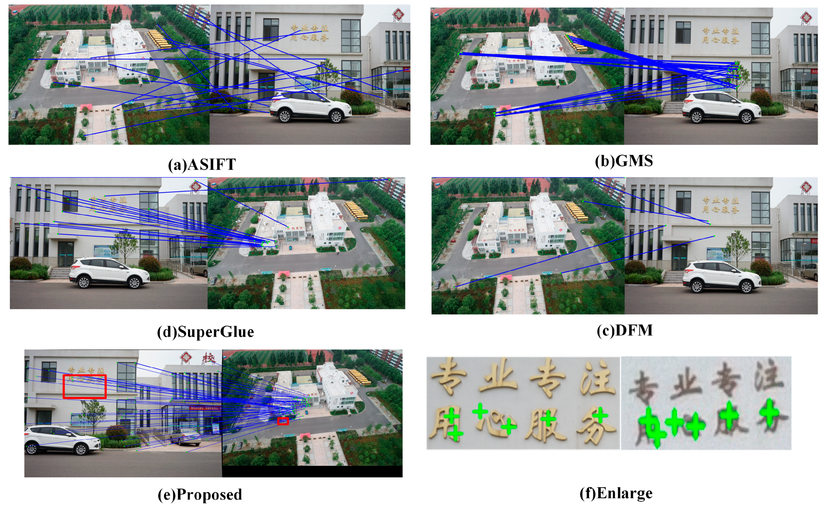
Figure 15.
Image feature-matching comparison on the hospital image in the Shandong University of Science and Technology dataset. (a–d) show the matching results of the ASIFT, GMS, DFM, and SuperGlue algorithms, respectively. (e) shows the matching result of the proposed algorithm, and (f) shows a magnified view of the matched feature points.
In the experiment on the SDUST-HOSP dataset, unfortunately, the method based on deep learning and the traditional method almost completely failed. The proposed method also faced some challenges. The quantitative results of the different methods are shown in Table 5. With an extreme difference in image scale, the proposed algorithm can still obtain enough inliers. As the representative result in Figure 15 shows, ASIFT, GMS, and DFM can hardly obtain enough matches. More matches are obtained by SuperGlue; however, the correspondence is not correct. The effect of the proposed method is also affected. The number of inliers and total matches are greatly reduced, but the matching accuracy remains stable.
Table 5.
Quantitative results of the different methods on dataset SDUST-HOSP.
3.3.3. Result of Image Reconstruction
Highly detailed 3D mesh models are usually reconstructed with aerial and terrestrial images. Different views of the image make the reconstruction result more complete. The integration of aerial and terrestrial images is the basis of combined reconstruction. However, in the experiments, ASIFT, GMS, and DFM can hardly obtain the tie points between the aerial and terrestrial images. Therefore, the terrestrial images with more detail cannot be integrated with aerial images, and their reconstructed models are similar to the models generated with only aerial images. The ASIFT, GMS, and DFM models are shown in Figure 16. The colorful box is a magnified view showing the details of the model. There is serious distortion at the bottom of the building, and the texture details of the building walls are poor.
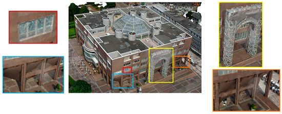
Figure 16.
Model generated after the aerial–terrestrial images were aligned by ASIFT, GMS, and DFM.
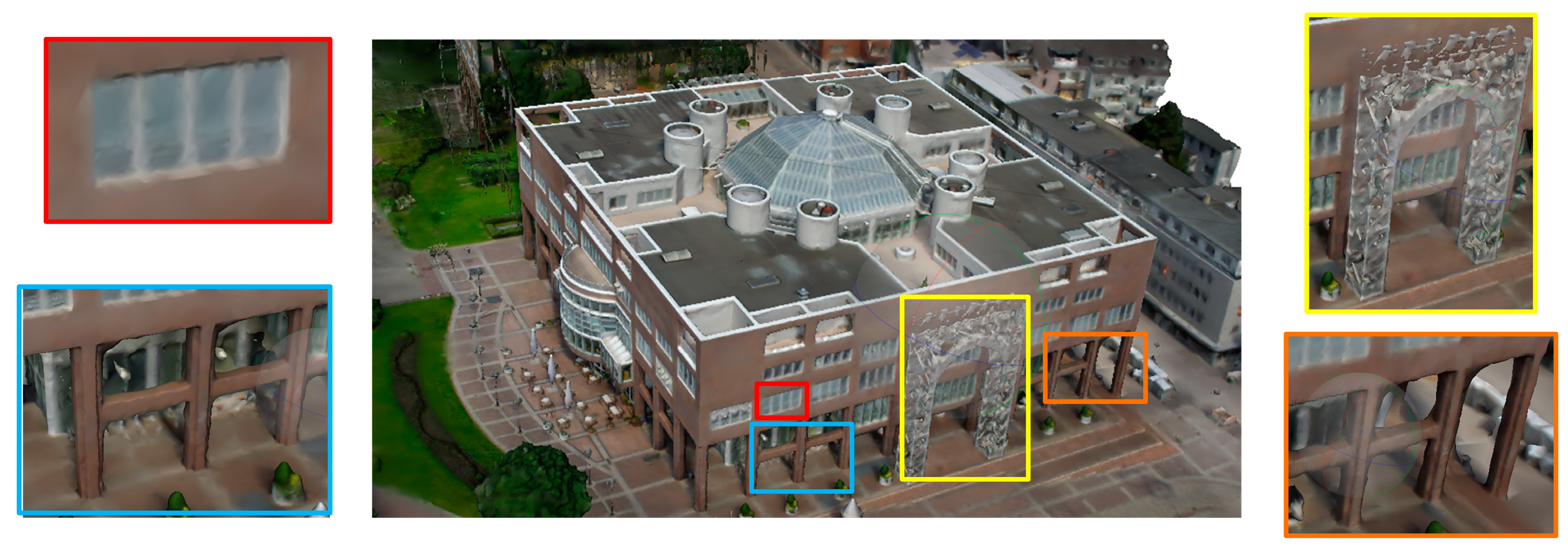
The matching effect of SuperGlue in cross-view aerial–terrestrial images is inferior to the effect of the proposed method; less tie points are obtained, and parts of the terrestrial images cannot be aligned with the aerial images, which makes the generated model lack some details. As shown by the representative result in Figure 17, the blue, yellow, and orange box areas of the models generated by SuperGlue are blurred and deformed. The model generated after aerial–terrestrial alignment by the proposed method is shown in Figure 18.
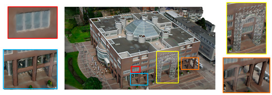
Figure 17.
The model generated after the aerial–terrestrial images were aligned by SuperGlue.
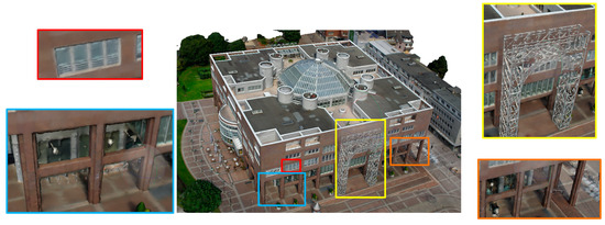
Figure 18.
The model generated after the aerial–terrestrial images were aligned by the proposed method.
3.3.4. Evaluation of the Effectiveness and Robustness of the Proposed Method
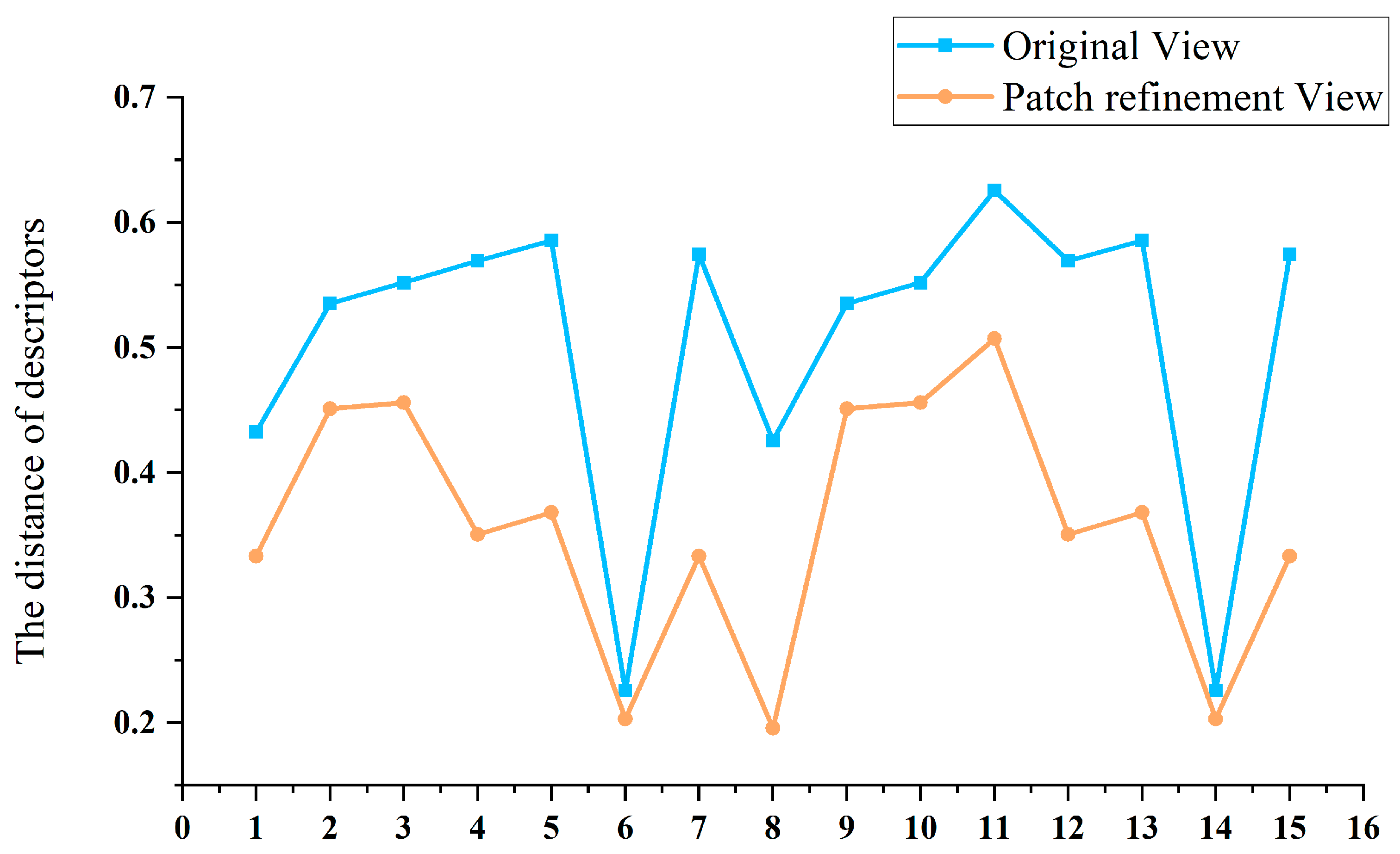
The descriptor variation distance is an index used to verify the effect of patch refinement. Taking image pair 8 from the Dort-Center dataset as an example, Figure 19 shows the change in the descriptor distance on the same feature matches before and after patch refinement.

Figure 19.
Analysis of changes in descriptor distances before and after view rectification.
In Figure 19, the matches with the same number on the horizontal axis share the same feature locations (the location distance is less than 2 pixels) on the images. This figure only shows 15 match results, the No. 6 and No. 14 matches are matched both in the original view and rectified view, and other matches fail in the original view. For the matches that are outliers in the original views but inliers in the rectified views, the descriptor distances decrease significantly.
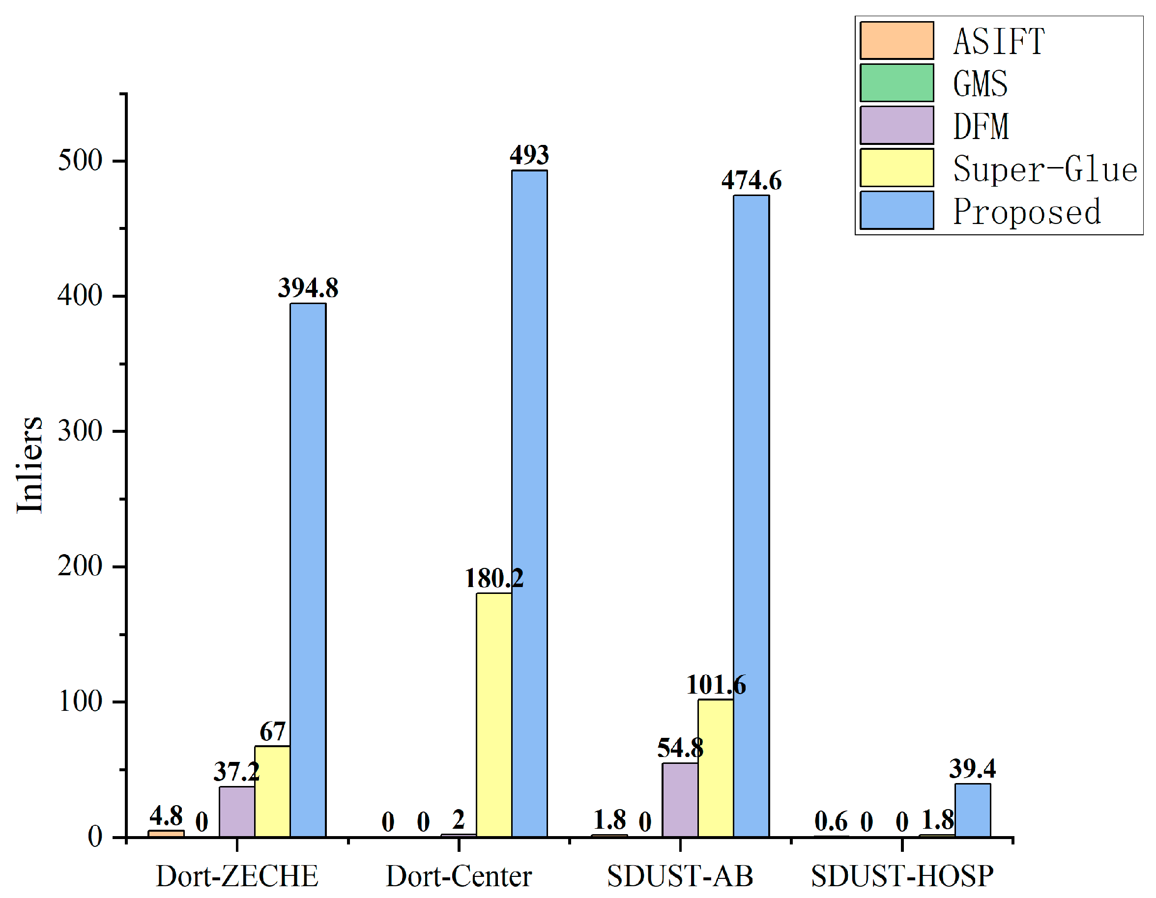
The reason for this may be that when transforming terrestrial-view and aerial-view images into the refined patch view, the geometric features are recovered and easily recognized, thereby leading to more similar match feature descriptors. This is helpful for increasing the number of inliers in the putative match set. Figure 20 shows a comparison of the mean number of correct matches (inliers) on the four datasets.
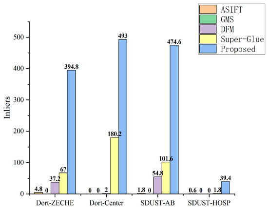
Figure 20.
Mean inliers of each dataset.
The experimental results demonstrate that the performance of the proposed aerial–terrestrial image-matching method is effective. The experiments on the Dortmund datasets verify that when the intersection angle of aerial–terrestrial images exceeds 60°, the matching effect of traditional methods almost fails; the mean matching accuracy of the deep learning method is slightly lower than that of the proposed method; however, the total number of inliers is substantially less than that of the proposed method. The experiments on the SDUST dataset show the robustness of the proposed method; it can obtain enough inliers without POS data.
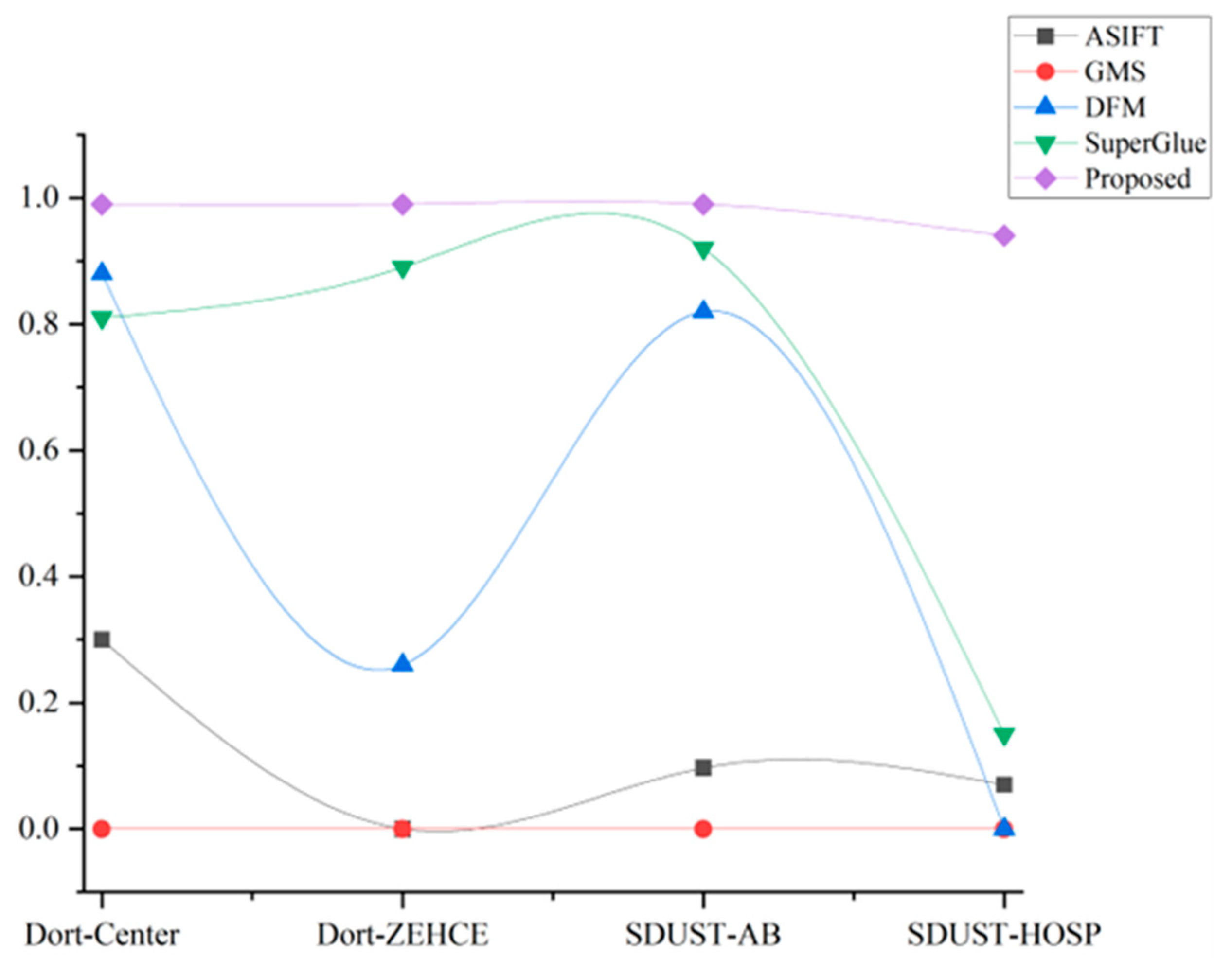
The number of inliers and matching accuracy of different algorithms on these datasets are shown in Figure 20 and Figure 21, respectively. These figures intuitively show the robustness and accuracy of the proposed algorithms when dealing with images with drastic changes in viewpoint and scale.

Figure 21.
Mean matching accuracy of each dataset.
4. Conclusions
In this paper, an approach to obtain tie points between terrestrial and aerial images is proposed. After variational patch refinement, the patches close to the surface of the object become a bridge between terrestrial and aerial images. The image perspective distortion and scale difference can be eliminated substantially by projecting onto a patch. The geometric property that is inherited from the point cloud can remove the outliers and improve the matching accuracy. Four datasets are used for quantitative analysis to evaluate the proposed approach.
In the experiments, although ASIFT and GMS have been optimized for cross-view images, because the intersecting angle of aerial–terrestrial image pairs usually exceeds 60°, the classical methods can hardly obtain correct tie points. For the deep-learning method, the robustness of DFM is not good, which may be because the buildings in the datasets have concave and convex structures. When dealing with nonplanar structures, the effect of DFM is poor. SuperGlue maintains high matching accuracy in most cases; however, the number of inliers in different image pairs varies greatly. For some image pairs, the correct matches are often less than 30. The robustness of SuperGlue is inferior to that of the proposed methods.
The results indicate that the proposed approach performs better than several state-of-the-art techniques in terms of both accuracy and the matching effect.
4.1. Contribution
The proposed method intends to solve the problem of severe perspective distortion and scale difference due to drastic changes in viewpoint. Patches are established and optimized by variational patch refinement so that they are close to the local tangent plane of the surface. Then, the differences in the image viewpoint, scale, and radiation between aerial oblique and terrestrial images are reduced or even eliminated. In addition, the patches inherit the geometry attribute of the point clouds, which can limit the workspace for feature matching and eliminate the outliers caused by the repetitive patterns using 3D similarity transformation. The significance of the proposed approach lies in its robustness and accuracy; it is almost unaffected by the convergent angle between aerial and terrestrial images and has few mismatches.
4.2. Limitations of the Proposed Method
The proposed patched-based terrestrial–aerial image-matching method still has the following limitations:
- Compared with traditional matching methods, the proposed method needs to build a patch based on images in the same view, which will increase the calculation time.
- This method rectifies the image scale difference by setting the size of the patch corresponding to the feature point based on GPS data. If there is no GPS assistance during image acquisition, the scale difference needs to be reduced by building an image pyramid on the patch.
- Occlusion is still a difficult problem; obscured parts of images usually cannot be used to generate correct point clouds, and it is difficult to maximize the photo-consistency between occluded images and normal images.
Optimization of the time complexity and the processing of occluded images are the directions of future research. Furthermore, although the proposed method can deal with the scale difference between aerial–terrestrial images, when the image scale difference is too large, the image resolution becomes a limiting factor of image matching, and super-resolution may be a solution.
Although the reconstruction results of the combination of aerial and ground images are highly detailed, in the high-frequency structure area, the reconstruction model is still blurred. Photometric stereo [37] and mesh refinement may be the proper methods to reconstruct high-quality mesh shapes.
Author Contributions
J.L. conceived the idea and designed the experiments.; H.Y. performed the experiments and analyzed the data.; H.Y. wrote the main manuscript.; J.L. and H.Y. reviewed the paper. Funding acquisition: P.L. and B.L. All authors have read and agreed to the published version of the manuscript.
Funding
This research was funded by the National Natural Science Foundation of China, grant number 42171439; Qingdao Science and Technology Demonstration and Guidance Project (grant no. 22-3-7-cspz-1-nsh); QingDao Key Laboratory for the integration and application of sea-land geographical information.
Data Availability Statement
Not applicable.
Conflicts of Interest
The authors declare no conflict of interest.
References
- Wu, B.; Xie, L.F.; Hu, H.; Zhu, Q.; Yau, E. Integration of aerial oblique imagery and terrestrial imagery for optimized 3D modeling in urban areas. ISPRS J. Photogramm. 2018, 139, 119–132. [Google Scholar] [CrossRef]
- Nex, F.; Remondino, F.; Gerke, M.; Przybilla, H.-J.; Bäumker, M.; Zurhorst, A. ISPRS benchmark for multi-platform photogrammetry. In Proceedings of the Joint Isprs Conference, Munich, Germany, 25–27 March 2015; pp. 135–142. [Google Scholar]
- Gao, X.; Shen, S.; Zhou, Y.; Cui, H.; Zhu, L.; Hu, Z. Ancient Chinese architecture 3D preservation by merging ground and aerial point clouds. ISPRS J. Photogramm. 2018, 143, 72–84. [Google Scholar] [CrossRef]
- Balletti, C.; Guerra, F.; Scocca, V.; Gottardi, C. 3D integrated methodologies for the documentation and the virtual reconstruction of an archaeological site. Int. Arch. Photogramm. Remote Sens. Spat. Inf. Sci. 2015, XL–5/W4, 215–222. [Google Scholar] [CrossRef]
- Jian, M.; Dong, J.; Gong, M.; Yu, H.; Nie, L.; Yin, Y.; Lam, K.M. Learning the Traditional Art of Chinese Calligraphy via Three-Dimensional Reconstruction and Assessment. IEEE Trans. Multimed. 2020, 22, 970–979. [Google Scholar] [CrossRef]
- Zhang, C.-S.; Zhang, M.-M.; Zhang, W.-X. Reconstruction of measurable three-dimensional point cloud model based on large-scene archaeological excavation sites. J. Electron. Imagining 2017, 26, 011027. [Google Scholar] [CrossRef]
- Ren, C.; Zhi, X.; Pu, Y.; Zhang, F. A multi-scale UAV image matching method applied to large-scale landslide reconstruction. Math. Biosci. Eng. 2021, 18, 2274–2287. [Google Scholar] [CrossRef] [PubMed]
- Rumpler, M.; Tscharf, A.; Mostegel, C.; Daftry, S.; Hoppe, C.; Prettenthaler, R.; Fraundorfer, F.; Mayer, G.; Bischof, H. Evaluations on multi-scale camera networks for precise and geo-accurate reconstructions from aerial and terrestrial images with user guidance. Comput. Vis. Image Underst. 2017, 157, 255–273. [Google Scholar] [CrossRef]
- Zhang, Y.; Ma, G.; Wu, J. Air-Ground Multi-Source Image Matching Based on High-Precision Reference Image. Remote Sens. 2022, 14, 588. [Google Scholar] [CrossRef]
- Zhu, Q.; Wang, Z.D.; Hu, H.; Xie, L.F.; Ge, X.M.; Zhang, Y.T. Leveraging photogrammetric mesh models for aerial-ground feature point matching toward integrated 3D reconstruction. ISPRS J. Photogramm. 2020, 166, 26–40. [Google Scholar] [CrossRef]
- Lowe, D.G. Distinctive image features from scale-invariant keypoints. Int. J. Comput. Vis. 2004, 60, 91–110. [Google Scholar] [CrossRef]
- Bay, H.; Ess, A.; Tuytelaars, T.; Van Gool, L. Speeded-up robust features (SURF). Comput. Vis. Image Underst. 2008, 110, 346–359. [Google Scholar] [CrossRef]
- Morel, J.-M.; Yu, G. ASIFT: A new framework for fully affine invariant image comparison. SIAM J. Imaging Sci. 2009, 2, 438–469. [Google Scholar] [CrossRef]
- Mikolajczyk, K.; Tuytelaars, T.; Schmid, C.; Zisserman, A.; Matas, J.; Schaffalitzky, F.; Kadir, T.; Gool, L.V. A Comparison of Affine Region Detectors. Int. J. Comput. Vis. 2005, 65, 43–72. [Google Scholar] [CrossRef]
- Xue, N.; Xia, G.S.; Bai, X.; Zhang, L.P.; Shen, W.M. Anisotropic-Scale Junction Detection and Matching for Indoor Images. IEEE Trans. Image Process. 2018, 27, 78–91. [Google Scholar] [CrossRef]
- Kushnir, M.; Shimshoni, I. Epipolar Geometry Estimation for Urban Scenes with Repetitive Structures. IEEE T. Pattern Anal. 2014, 36, 2381–2395. [Google Scholar] [CrossRef]
- Zhang, Q.; Li, Y.J.; Blum, R.S.; Xiang, P. Matching of images with projective distortion using transform invariant low-rank textures. J. Vis. Commun. Image Represent. 2016, 38, 602–613. [Google Scholar] [CrossRef]
- Yue, L.W.; Li, H.J.; Zheng, X.W. Distorted Building Image Matching with Automatic Viewpoint Rectification and Fusion. Sensors 2019, 19, 5205. [Google Scholar] [CrossRef]
- Hu, H.; Zhu, Q.; Du, Z.Q.; Zhang, Y.T.; Ding, Y.L. Reliable Spatial Relationship Constrained Feature Point Matching of Oblique Aerial Images. Photogramm. Eng. Rem. S. 2015, 81, 49–58. [Google Scholar] [CrossRef]
- Jiang, S.; Jiang, W.S. On-Board GNSS/IMU Assisted Feature Extraction and Matching for Oblique UAV Images. Remote Sens. 2017, 9, 813. [Google Scholar] [CrossRef]
- Fanta-Jende, P.; Gerke, M.; Nex, F.; Vosselman, G. Co-registration of Mobile Mapping Panoramic and Airborne Oblique Images. Photogramm. Rec. 2019, 34, 149–173. [Google Scholar] [CrossRef]
- Shan, Q.; Wu, C.; Curless, B.; Furukawa, Y.; Hernandez, C.; Seitz, S.M. Accurate Geo-Registration by Ground-to-Aerial Image Matching. In Proceedings of the 3DV, Tokyo, Japan, 8–11 December 2014; pp. 525–532. [Google Scholar]
- Altwaijry, H.; Belongie, S. Ultra-wide Baseline Aerial Imagery Matching in Urban Environments. In Proceedings of the British Machine Vision Conference 2013, Bristol, UK, 9–13 September 2013; p. 15.11. [Google Scholar]
- Yi, K.M.; Trulls, E.; Lepetit, V.; Fua, P. LIFT: Learned Invariant Feature Transform. In Proceedings of the European Conference on Computer Vision, Amsterdam, The Netherlands, 11–14 October; Springer: Cham, Switzerland, 2016; pp. 467–483. [Google Scholar]
- Zhang, X.; Yu, F.X.; Karaman, S.; Chang, S. Learning Discriminative and Transformation Covariant Local Feature Detectors. In Proceedings of the 2017 IEEE Conference on Computer Vision and Pattern Recognition (CVPR), Honolulu, HI, USA, 21–26 July 2017; pp. 4923–4931. [Google Scholar]
- Efe, U.; Ince, K.G.; Alatan, A.A.; Soc, I.C. DFM: A Performance Baseline for Deep Feature Matching. In Proceedings of the CVPR, Virtual Event, 19–25 June 2021; pp. 4279–4288. [Google Scholar]
- DeTone, D.; Malisiewicz, T.; Rabinovich, A.; IEEE. SuperPoint: Self-Supervised Interest Point Detection and Description. In Proceedings of the CVPR, Salt Lake City, UT, USA, 18–22 June 2018; pp. 337–349. [Google Scholar]
- Sarlin, P.E.; DeTone, D.; Malisiewicz, T.; Rabinovich, A.; IEEE. SuperGlue: Learning Feature Matching with Graph Neural Networks. In Proceedings of the CVPR, Virtual Event, 14–19 June 2020; pp. 4937–4946. [Google Scholar]
- Pautrat, R.; Larsson, V.; Oswald, M.; Pollefeys, M. Online Invariance Selection for Local Feature Descriptors. In Proceedings of the ECCV, Glasgow, UK, 23–28 August 2020; Springer: Cham, Switzerland, 2020; pp. 707–724. [Google Scholar]
- Simonyan, K.; Zisserman, A. Very Deep Convolutional Networks for Large-Scale Image Recognition. arXiv 2014, arXiv:1409.1556. [Google Scholar]
- Jin, Y.; Mishkin, D.; Mishchuk, A.; Matas, J.; Fua, P.; Yi, K.M.; Trulls, E. Image Matching Across Wide Baselines: From Paper to Practice. Int. J. Comput. Vis. 2021, 129, 517–547. [Google Scholar] [CrossRef]
- Moulon, P.; Monasse, P.; Perrot, R.; Marlet, R. OpenMVG: Open Multiple View Geometry. In Proceedings of the Reproducible Research in Pattern Recognition, Virtual Event, 11 January 2017; Springer: Cham, Switzerland, 2017; pp. 60–74. [Google Scholar]
- Mikolajczyk, K.; Schmid, C. A performance evaluation of local descriptors. IEEE T. Pattern Anal. 2005, 27, 1615–1630. [Google Scholar] [CrossRef] [PubMed]
- Bian, J.W.; Lin, W.Y.; Matsushita, Y.; Yeung, S.K.; Nguyen, T.D.; Cheng, M.M. GMS: Grid-based Motion Statistics for Fast, Ultra-robust Feature Correspondence. In Proceedings of the CVPR, Honolulu, HI, USA, 21–26 July 2017; pp. 2828–2837. [Google Scholar]
- Sarlin, P.E.; DeTone, D.; Malisiewicz, T.; Rabinovich, A. SuperGlue github repository. In Proceedings of the CVPR, Virtual Event, 14–19 June 2020; Available online: https://github.com/magicleap/SuperGluePretrainedNetwork (accessed on 5 December 2022).
- Efe, U.; Ince, K.G.; Alatan, A.A.; Soc, I.C. DFM github repository. In Proceedings of the CVPR, Virtual Event, 19–25 June 2021; Available online: https://github.com/ufukefe/DFM (accessed on 5 December 2022).
- Ju, Y.; Shi, B.; Jian, M.; Qi, L.; Dong, J.; Lam, K.-M. NormAttention-PSN: A High-frequency Region Enhanced Photometric Stereo Network with Normalized Attention. Int. J. Comput. Vis. 2022, 130, 3014–3034. [Google Scholar] [CrossRef]


Disclaimer/Publisher’s Note: The statements, opinions and data contained in all publications are solely those of the individual author(s) and contributor(s) and not of MDPI and/or the editor(s). MDPI and/or the editor(s) disclaim responsibility for any injury to people or property resulting from any ideas, methods, instructions or products referred to in the content. |
© 2023 by the authors. Licensee MDPI, Basel, Switzerland. This article is an open access article distributed under the terms and conditions of the Creative Commons Attribution (CC BY) license (https://creativecommons.org/licenses/by/4.0/).