Article

Spectral Simulation and Error Analysis of Dusty Leaves by Fusing the Hapke Two-Layer Medium Model and the Linear Spectral Mixing Model

1
Institute for Geoinformatics & Digital Mine Research, Northeastern University, Shenyang 110819, China
2
Key Laboratory of Ministry of Education on Safe Mining of Deep Metal Mines, Northeastern University, Shenyang 110819, China
*
Author to whom correspondence should be addressed.
Remote Sens. 2023, 15(5), 1220; https://doi.org/10.3390/rs15051220
Submission received: 3 January 2023 / Revised: 18 February 2023 / Accepted: 20 February 2023 / Published: 22 February 2023
(This article belongs to the Section Environmental Remote Sensing)

Abstract

:
The Hapke two-layer medium model is an efficient way of simulating the spectra of dusty leaves. However, the simulation accuracy is low when the amount of dustfall is small. To solve this problem, we introduced the dust coverage factor and the linear spectral mixing model, to improve the accuracy of the Hapke two-layer medium model. Firstly, based on the assumption of spherical dust particles, the arrangement and accumulation mode of the particles were set, and the coverage factor and accumulation thickness of particles in the leaf area were calculated. Then, the coverage factor was used as an abundance. Endmembers were the spectra of dust-free leaves (measured) and dust-covered leaves (simulated by model), and the final simulated spectra were calculated using linear spectral mixing theory. This study presents the following findings: (1) When the coverage factor was calculated using the exponential model, the maximum difference between the corrected simulated spectra and the measured spectra was 3.4%, and the maximum difference between the original simulated spectra and the measured spectra was 15.2%. The accuracy of the corrected spectra is much higher than that of the original simulated spectra. (2) In this study, the physical thickness and optical thickness calculated by the Hapke two-layer medium model are equivalent, which is quite different from the actual dust accumulation. When the linear spectral mixing model is introduced, to modify the simulation value when the number of dust particles accumulated is less than one layer, the spectral endmember value of the simulated dust leaf is replaced by the simulation spectrum when the number of dust particles accumulated is exactly one layer. The calculated cor-rection spectrum has high rationality and credibility. This finding may be beneficial for monitoring amounts of dustfall accurately using remote sensing in mining areas.

1. Introduction

Dust diffusion and deposition are widely considered important factors affecting the ecological environment [1]. Sources of dust particles include sandstorms [2,3], volcanic eruptions (ash) [4], mining operations [5], industrial production [6], energy consumption [7,8], urban activities [9], etc. Anthropogenic activities lead to the release of a huge amount of dust, and the problems of such dust pollution are well known and of serious concern. For example, in opencast mining [10], a large amount of dust is generated in excavation and loading [11,12,13]. In the transportation of minerals [14,15], dust is generated by the repeated rolling of wheels on the ground, and vehicle exhaust contains particulate matter [16]; exhaust gas increases the diffusion range of dust and not only endangers human life and health [17,18,19] but also causes serious damage to the surrounding environment [20,21]. Therefore, it is necessary to monitor dust pollution in mines, to guide the management of dust dispersion and dust pollution.
Remote sensing monitoring has technical advantages, such as a large monitoring range and high efficiency, and it is one of the most common means of monitoring the environment and vegetation in mining areas [22]. When dust settles on the surface of a leaf, via wind and gravity, it causes a change in the leaf spectrum [23,24]. The detection of dusty leaf spectra can be used to calculate dust pollution levels in mining areas, so it is necessary to measure and study the spectra of dusty leaves. Usually, there are difficulties in obtaining the spectra of dusty leaves [25], while pure dust spectra and dust-free leaf spectra are easier to obtain. Therefore, it is more convenient to calculate dust pollution levels by using the dust spectra of vegetation through modeling or simulation, and this work can provide basic data, and an evaluation basis for the assessment of regional ecological environments [26].
There are many methods used to simulate vegetation spectra, among which the SAIL model is a canopy-scale radiative transfer model that is suitable for simulating the spectral bi-directional reflectance (BRDF) characteristics of a uniform vegetation population, by simulating the interaction between incident radiation and a uniform medium and by considering multiple scattering factors [27]. The PROSPECT model is a multilayer flat plate model based on the radiation transfer model at the leaf level, which is used to calculate the isotropic scattering of the leaf structure [28]. By combining the SAIL model and the PROSPECT model, the PROSAIL model can be utilized to calculate the vegetation canopy spectrum and various important biochemical parameters of leaves. It is also the most widely used radiative transmission model for simulating vegetation canopy spectra [29,30]. DART is one of the most comprehensive and complex 3D radiation transfer models available [31]. It can construct natural or urban surface scenes from geomorphic data, and simulate surface and atmospheric radiation transmission processes from ultraviolet to thermal infrared [32]. At the canopy scale, the above models are more accurate in simulating or inverting the chlorophyll of vegetation in 3D radiation transfer. However, at the leaf scale, when the leaf and dust particles accumulate on the surface of the leaf forming a two-layer or multilayer medium, the above models cannot meet the requirements. Therefore, the Hapke two-layer medium model is introduced in this study to calculate the reflectivity of the two-layer medium of leaf and dust. The Hapke two-layer medium model was proposed by Hapke [33,34]. It has the advantages of being a simple solution, having high precision, and easy inversion [35]. However, the Hapke two-layer medium model cannot accurately calculate the simulated spectra when the amount of dust deposited is small. In this case, using the model to simulate the spectra of dusty leaves would produce a large error. Therefore, the model needs to be fused to obtain more accurate simulated spectra.
The purpose of this study is to fuse the Hapke two-layer medium model and the linear spectral mixing model so that the model can accurately simulate dusty leaf spectra when the amount of dust is small. The findings of the study may be used to support the retrieval of dustfall in mining areas.

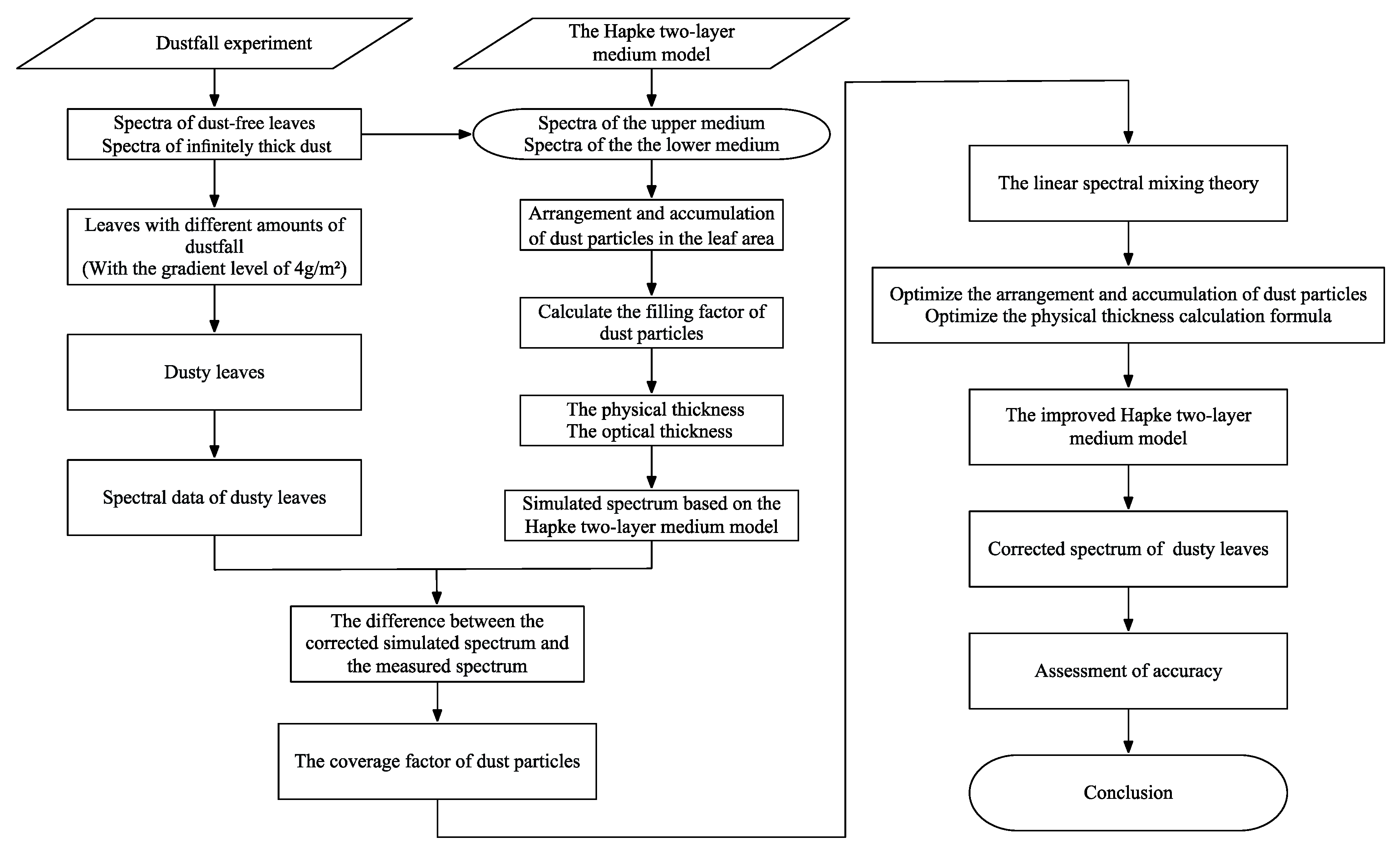
2. Data, Methods, and Method Optimization

In this paper, dust accumulation on the leaf and leaf surface was simplified into a two-layer medium model, and the overall reflectivity of the whole model was calculated according to different amounts of dustfall. The technical route is shown in Figure 1. According to Figure 1, first, a dustfall experiment was performed (with a gradient level of 4 g/m2), and spectral data of dusty leaves were obtained. The spectral data of dust-free leaves were used as the reflection spectra of the lower medium in the Hapke two-layer medium model. The infinitely thick dust spectrum was used as the Hapke upper medium reflection spectrum. Then, the filling factor was calculated based on the accumulation and arrangement of dust particles, and the calculated physical thickness and optical thickness were substituted into the Hapke bilayer dielectric model formula to calculate the simulated spectrum. Due to the large error in the obtained simulated spectrum, we further calculated the coverage of dust particles in the leaf region, introduced the linear spectral mixing model to correct the error, and achieved good results.

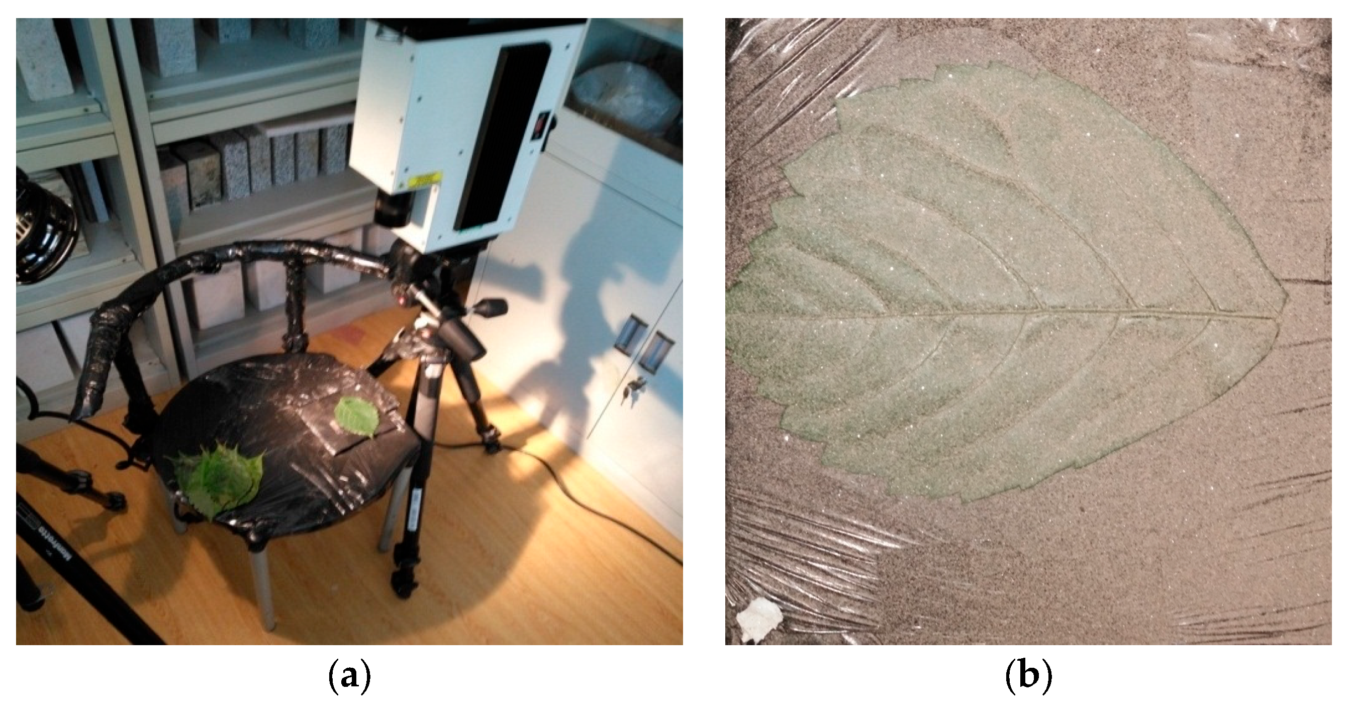
2.1. Data (Measured Spectral Data)

An SVC HR-1024 spectrometer was used to collect the spectral information of the samples, which was produced by Spectral Vista in the United States, with a spectral detection range of 350–2500 nm, a spectral resolution of 3.5–9.5 nm, and a channel number of 1024. Dust samples were collected from the tailings pond of the Qidashan Iron Mine of the Anshan Iron and Steel Mining Company. The dust particles were analyzed by chemical detection in the pattern test at Northeastern University, and their composition content is shown in Table 1.
Due to the wide distribution of particle sizes in dust samples, in order to simplify the calculation process in the experiment, dust particles with a single particle size (60 um) were selected as dust removal experimental samples, through artificial control.
Leaf spectra measurements and leaf dustfall experiments were conducted at the graduate school of Northeastern University. The leaves of Parthenocissus tricuspidata, commonly found in the school, were selected for the experiment. In order to ensure the freshness of the leaf samples, and eliminate the influence of water loss, leaf samples were picked before the experiment in the morning.
Firstly, the leaf spectrum measurement experiment was carried out, the experimental setup is shown in Figure 2a. The light source was a halogen lamp, with a height angle of 60° and a distance of 50 cm from the target. The measurement time of the spectrometer was 2 s. A 4° lens was used, with the leaf positioned directly below the lens, and the lens height from the leaf was set to 55 cm, to ensure that the leaf filled the field of view. The spectral curves of 32 sample leaves were measured in turn.
Then, the leaf dustfall experiment was carried out, and Figure 2b shows a leaf covered by dust particles after spraying a certain amount of dust during the experiment. In this study, dusty leaves with different dustfall amounts were obtained by adding quantitative dust to the leaf surface successively, and spectral data of dusty leaves with different dustfall amounts were measured. The specific operation consisted of successively spraying a fixed quantity of dust (4 g/m2) onto a dust-free leaf, with the upper limit of dust addition being 248 g/m2. After each addition of dust, the dusty leaf spectral data under the dust magnitude were measured, until all the spectral data between 0 and 248 g/m2 had been measured.

2.2. Theoretical Basis

2.2.1. Physical Thickness and Optical Thickness

Optical thickness is usually defined as the integration of the extinction coefficient in the vertical direction. Some researchers define the optical thickness of a path in the scattering medium as the dimensionless line integral of the extinction coefficient along the path. The calculation formula is as follows:
τ 0 = s   E s d s ,
where τ 0 is the optical thickness and E(s) is the extinction coefficient.
The calculation formula of optical thickness can be further simplified, and can be written as the product of the extinction coefficient and physical thickness, given by Equation (2):
τ 0 = E · t ,
where t is the physical thickness and E is the extinction coefficient.
Johnson [36] rewrote the optical thickness calculation formula based on Hapke’s paper [34], and the rewritten optical thickness calculation equation is Equation (3):
τ 0 = 3 t ln p / 2 d ,
where t is the physical thickness, p is the fractional pore space in the coating (equal to 1 minus the filling factor), and d is the dust grain size.

2.2.2. The Hapke Two-Layer Medium Model

For the Hapke two-layer medium model, if the upper layer is infinitely thick, the diffusive reflectance is calculated by Equation (4):
r U = 1 γ / 1 + γ ,
By transforming Equation (4), the albedo factor, γ, can be written as Equation (5):
γ = 1 r U / 1 + r U ,
The Hapke model diffusive reflectance, r 0 , of the system is given by Equation (6) [34]:
r 0 = r U 1 + 1 r U r L r U 1 r L r U e 4 γ τ 0 / 1 + r U r L r U 1 r L r U e 4 γ τ 0   ,
where r U is the diffuse reflectance of the upper medium and r L is the diffuse reflectance of the lower medium. In the simulation calculation, r U was taken as the spectral reflectance of infinitely thick dust, and r L was taken as the measured spectral value of the dust-free leaves. By substituting the corresponding parameters into Equation (6), to calculate the total reflectance, the simulated reflectance spectrum of this model can be obtained.

2.3. The Fusion of the Hapke Two-Layer Medium Model and the Linear Spectral Mixing Model

In real deposited dust particles, the arrangement and accumulation are usually complicated. Generally speaking, dust accumulation can be regarded as a probabilistic model, and different forms of dust accumulation cause different simulation results, which are reflected in the calculation of equivalent physical thickness. Due to changes in the equivalent physical thickness caused by accumulation and arrangement, the corresponding optical thickness also changes, so the Hapke two-layer medium model simulation results are slightly different. When the amount of dustfall gradually increases, the area covered by dust particles on the leaf surface also gradually increases. The physical thickness used in the Hapke two-layer medium model simulation is an equivalent calculation method. When the dust particles do not completely cover the leaf area, the overall thickness is equivalent to the thickness of a thin layer. However, in actual dust deposition, even if the dust particles do not completely cover the leaf area, the dust thickness is greater than or equal to the particle size. Therefore, the Hapke two-layer medium model simulation error mainly requires correction when dust particles do not completely cover the leaf area. The formula for the equivalent physical thickness corresponding to the arrangement and accumulation of dust particles is given in this section, and the dust coverage factor is introduced to correct the spectral reflectance simulated by the Hapke two-layer medium model when particles do not completely cover the leaf area.

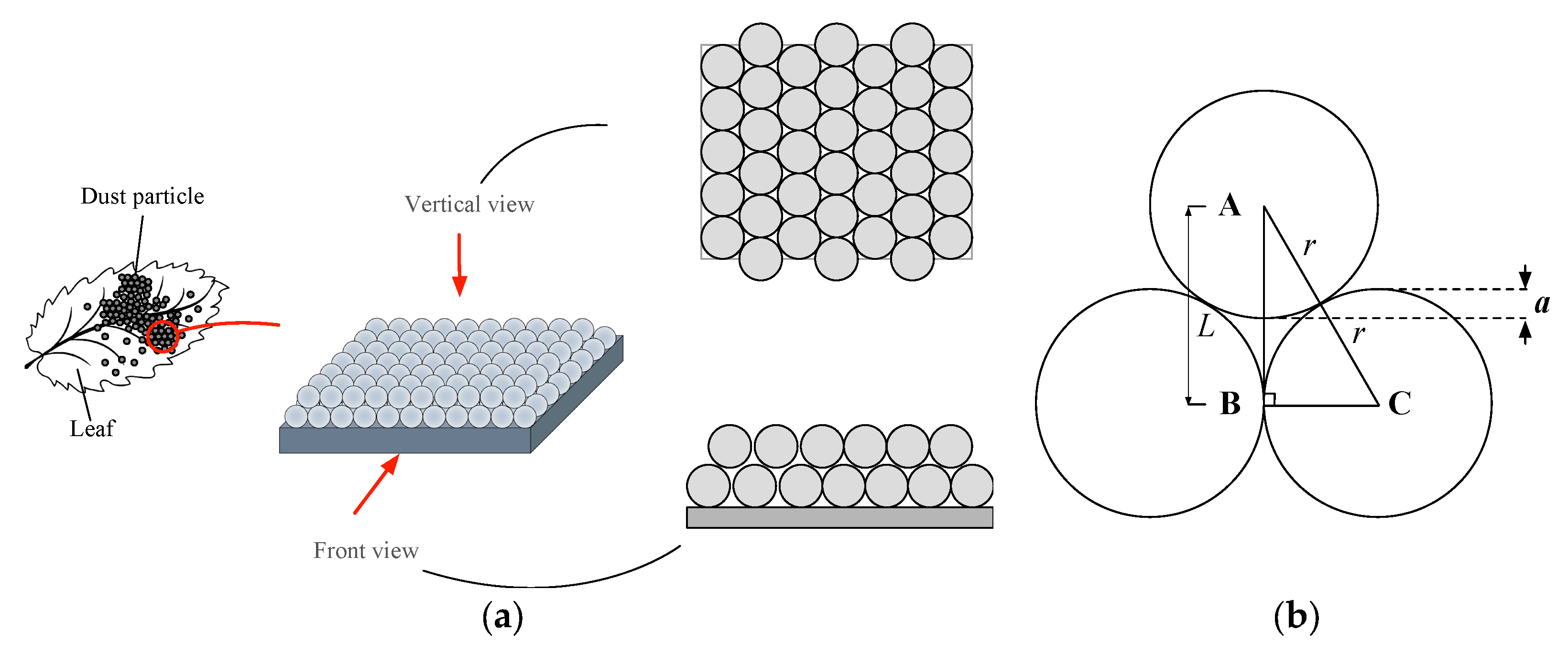
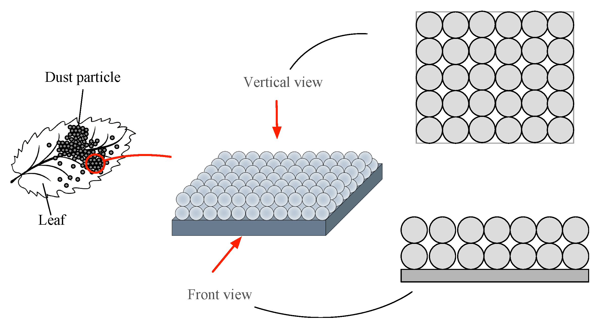
2.3.1. Arrangement and Accumulation of Dust Particles

In this study, the arrangement of dust particles has an impact on the dust coverage factor. Specifically, when the arrangement is close, the number of particles required increases, and the dust coverage factor is greater. When the arrangement is sparse, the number of dust particles is small, and the dust coverage factor is small. In addition, different particle accumulation modes also affect the calculated value of the filling factor. Different dust accumulation modes in the longitudinal direction cause an increase or decrease in the filling factor. This firstly changes the physical thickness calculation method, which directly affects the optical thickness, resulting in a change to the calculated value of the optical thickness and a change to the Hapke two-layer medium model simulation value. It also leads to a change in the filling factor calculation value: When the arrangement is tight, the multilayer particles are stacked, and the filling factor is small; otherwise, the filling factor becomes larger. The calculation deviation caused by the arrangement and accumulation of the above dust must be considered; thus, they need to be calculated in detail for systematic study and analysis.
The experiment treated all particles as ideal spheres, assuming that a single dust particle had a radius of r (units of cm) and a mass of m (units of g). The dust particles of iron tailings used in this study were taken from iron tailings in Qidashan, and the true density ρp of the iron tailings dust was 2.744   g / cm 3 . The mass of a single dust particle is given by the following formula:
m = ρ · v = ρ p × 4 π 3 × d 2 3 ,
When dust particles settled beside each other until they covered the entire leaf area, their distribution trend was similar to that in Figure 3a. In this case, in order to obtain the total number of dust particles forming a full layer, it is necessary to calculate the value of a first, so that the length of each pair of particles when they are close together can be calculated, and the number of particles per unit area can be calculated. Figure 3b shows the geometric relationship between a and the particles when they are accumulated or arranged. This is also true for the case of dust particle accumulation; given the value of a, the physical thickness at the time of accumulation can also be calculated.
According to the arrangement and accumulation in Figure 3a, the calculation process of a is given by Equation (8) [37].
a = r + r 3 r = 0.268 r = 0.134 d ,
Based on the arrangement of dust particles in Figure 3a, the number of particles per unit area (cm2) is given by Equation (9).
N T = 1.155 / d × 1 / d = 1.155 / d 2 ,
where N T is the number of particles per unit area (cm2) and d is the dust grain size.
The filling factor refers to the degree to which the bulk material is filled by its particles in a certain bulk volume. In this study, the filling factor refers to the degree of filling by dust particles per unit volume of the leaf surface, which reflects the void rate generated when the particles are filled per unit volume. The filling factor based on this arrangement can be calculated using Equation (10).
φ = 1 N T 3 2 × 4 3 π × d 3 8 1 × 1 × 1 = 1 0.65 = 0.35 ,
According to Equations (3) and (6), the filling factor can affect the optical thickness calculation of the dust particles, which further affects the spectral values simulated by the model. Therefore, the change in the arrangement and accumulation of dust particles will make the calculation value of the filling factor change accordingly, and eventually affect the accuracy of the model simulation spectrum.
The number of dust particles on the leaves increases with the increase in dustfall amount. The calculation of the equivalent physical thickness of the dust medium is related to the accumulation method. We next introduce the calculation method for the equivalent physical thickness of the dust medium.
In this study, we make a corresponding simplification of the equivalent physical thickness of the stacking process. The calculation of equivalent physical thickness is divided into two cases: when the number of accumulation layers is less than one layer, and when it is more than one layer. The specific steps are as follows:
  • When the accumulation of dust particles is less than one layer, the calculation process for the equivalent physical thickness is as follows:
Firstly, the calculation formula of the physical thickness is given, as shown in Equation (11).
t = N L · d ,
The calculation of the accumulation layer number, N L , is the ratio of M to the total weight of particles per unit area, as shown in Equation (12):
N L = M ( 100 × N T ) 2 × m   ,
where M is the amount of dustfall, m is the mass of a single dust particle, and N T is the number of particles per unit area (cm2).
By simplifying the above formula, Equation (13) can be obtained.
N L = M ( 100 × N T ) 2 × ρ p × 4 π 3 × d 2 3 = 6 M N T · ρ p · d 3 × 10 4   ,
By combining Equations (11) and (13), the calculation formula of the equivalent physical thickness can be obtained as shown in Equation (14).
t = N L · d = 6 M N T · ρ p · d 2 × 10 4   ,
2.
When the accumulation layer of dust particles is one layer, there are two parts to calculating the equivalent physical thickness of the dust medium.
  • t   < ( d + a ) :
t = d ,
  • ( d + a ) < t < ( 2 d a ) :
t = d + N L 1 × d a ,
The equivalent physical thickness of the dust medium at more than two layers is calculated in the same way; thus, it is not repeated here.

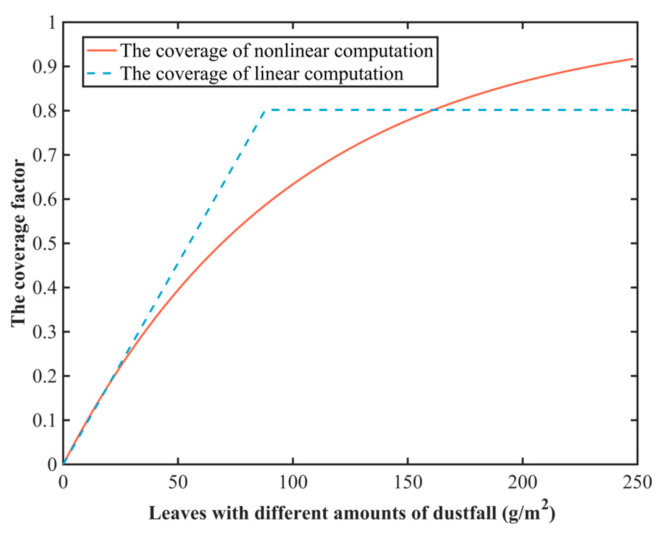
2.3.2. The Dust Coverage Factor

The dust coverage factor is introduced to correct the Hapke two-layer medium model’s simulated spectrum. The correction formula is based on linear spectral mixing theory. The composition of the mixed spectrum is the endmembers, and the proportion of the end element is the abundance; that is, the corrected spectrum is the linear combination of the endmember spectrum and its abundance. In this study, endmember spectra are the dust-free leaf spectra and the dusty leaf spectra simulated by the Hapke two-layer medium model with different amounts of dustfall. The spectral abundance of dust-free leaves is the ratio of the area not covered by dust to the total area, and the spectral abundance of the Hapke two-layer medium model simulation is the dust coverage factor. To summarize, the correction formula can be given by Equation (17).
R = 1 f d × r L + f d × R H a p k e ,
where r L is the measured spectrum of the dust-free leaves, f d is the dust coverage factor, and R H a p k e is the simulated spectrum of the corresponding amounts of dustfall.
The formula for calculating f d is based on the number of layers of particles piled up above, which is shown in Equation (18).
f d = S c S = 100 × N T 2 × N l a y × π · d 2 2 100 × 100 = π N L 4 × 1.155 ,
For Equation (18), it should be noted that f d does not change when the dust particles are distributed in one layer in the leaf area.
However, in the actual experiment, there is a nonlinear law between the dust coverage factor and the different amounts of dustfall, so it is necessary to further match the dust coverage factor to reality as closely as possible.
Neil S. Beattie [38] obtained a mathematical model of particle accumulation through experiment, which can better reflect real particle accumulation situations. The calculation method is given in Equation (19).
f d = 1 e N L ,
where f d is the proportion of the area covered by dust particles in the total area and N L is the number of the accumulation layers of dust particles.
Thus, Equation (17) can be rewritten as Equation (20).
R = 1 f d × r L + f d × R H a p k e ,
The basic principle of the Hapke two-layer medium model simulation value correction formula, R′, is based on the idea of the linear spectral mixing model. When the particles are not fully spread, a part of the leaf area must not be covered by dust, so this part of the area should show the characteristics of a dust-free spectrum. The remaining area is the dust-covered area, which should show the actual spectral characteristics of pure dust. Therefore, when the number of dust layers is less than one, the spectrum of the uncovered area should be the spectrum of the dust-free leaf, while the spectrum of the covered area should be the spectrum of the covered area with a full layer. At this point, Equation (20) can be further rewritten.
When dust particles do not completely cover the leaf area, the R H a p k e in Equation (20) is changed to R H , and a new correction formula is obtained in this case:
R = 1 f d × r L + f d × R H ,
where R H is the simulated spectrum under the corresponding amount of dustfall when the number of dust accumulation layers is one.
The correction formula for the accumulation of more than one layer of dust particles is the corresponding simulated reflectance, R H a p k e , as shown in Equation (22).
R = 1 f d × r L + f d × R H a p k e ,

3. Results

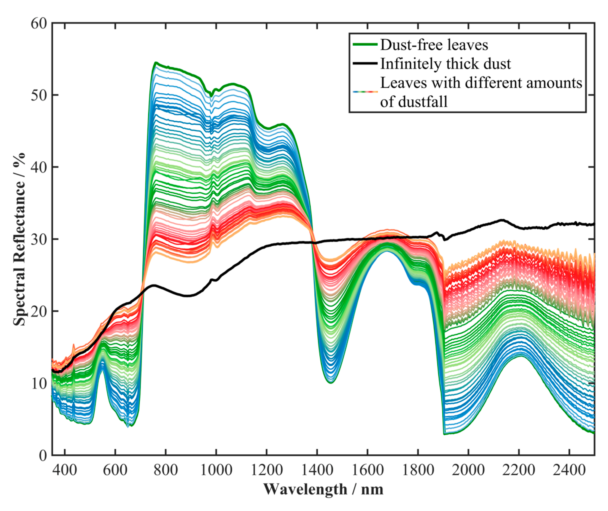
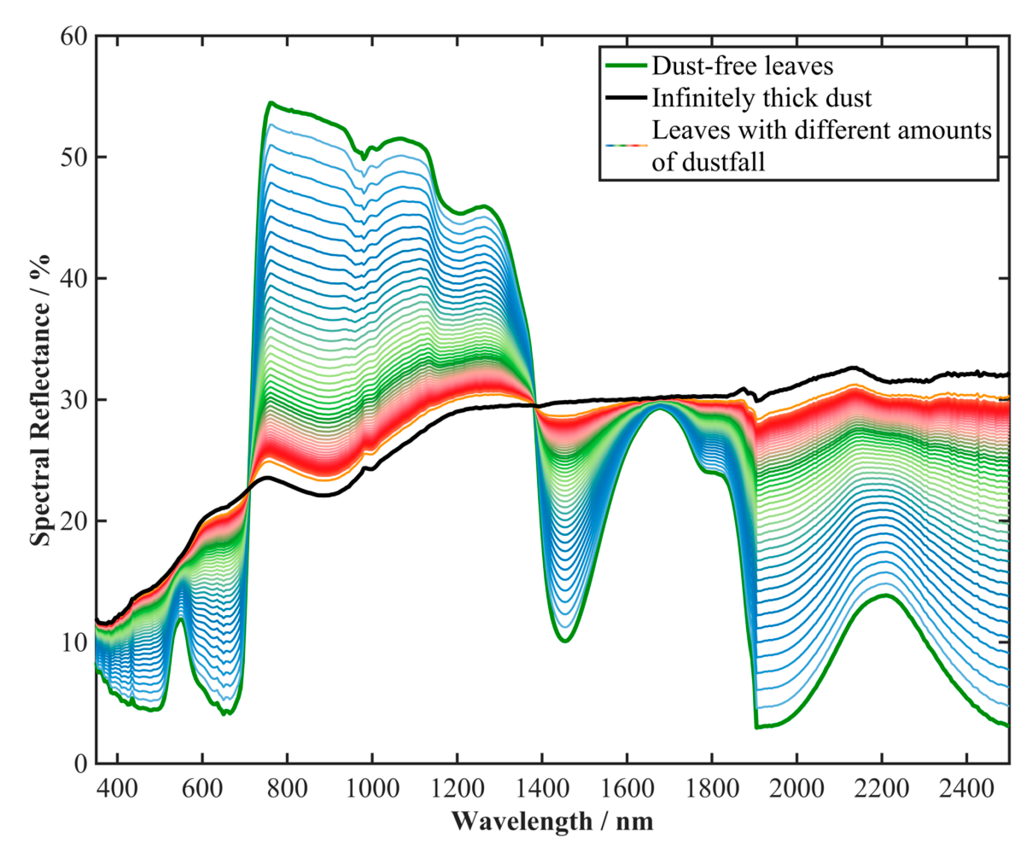
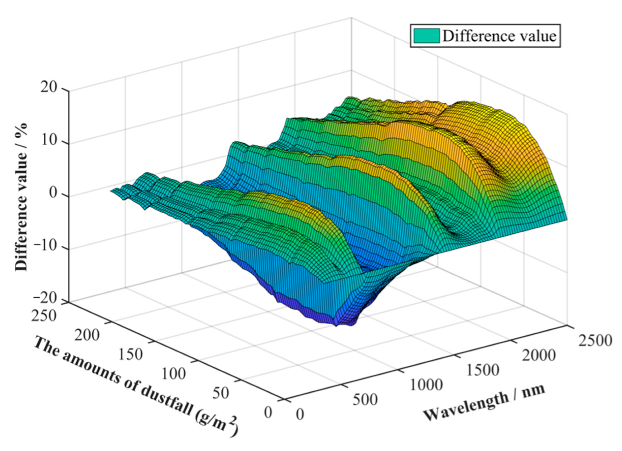
3.1. Measured Spectra and Simulated Spectra by Using Hapke Two-Layer Medium Model Directly

The measured spectral curves of leaves with different amounts of dustfall is shown in Figure 4. The results show that, as the amount of dustfall increases, the spectral curve of dusty leaves approaches that of dust. Taking one of the two experimental leaves as an example (Figure 4), in the ranges of 380–710 nm and 1420–1570 nm, the reflectance of dusty leaves is higher than that of non-dusty leaves. The reflectance of dusty leaves increases as dustfall amounts increase. The crest flattens out at 559 nm. In the range of 710–1420 nm, the reflectance of dust-free leaves is higher than that of dusty leaves, and the reflectance decreases with an increase in dustfall amount. In the range of 1570–1900 nm, the reflectance of dust-free leaves is lower than that of dusty leaves, and the reflectance increases with an increase in dustfall amount.
The Hapke two-layer medium model simulates the spectral curves of leaves with different amounts of dustfall. The results are shown in Figure 5. By calculating the difference between the simulated spectral value and the measured spectrum, the two-dimensional surface diagram of the difference, shown in Figure 6, could be calculated. In the range of 720–1370 nm, the difference is negative, and the simulated spectral reflectance is lower than the measured spectral reflectance. In the ranges of 350–720 nm and 1370–2500 nm, the difference is positive, and the simulated spectral reflectance is higher than the measured spectral reflectance. When the amount of dustfall is less than what is needed to cover the first layer, the difference widens as the amount of dustfall increases. When the amount of dust is 76 g/m2 and the wavelength is 2500 nm, the greatest difference is about 15.2%. When above the amount of dustfall required for one layer, the difference decreases as the amount of dustfall increases.

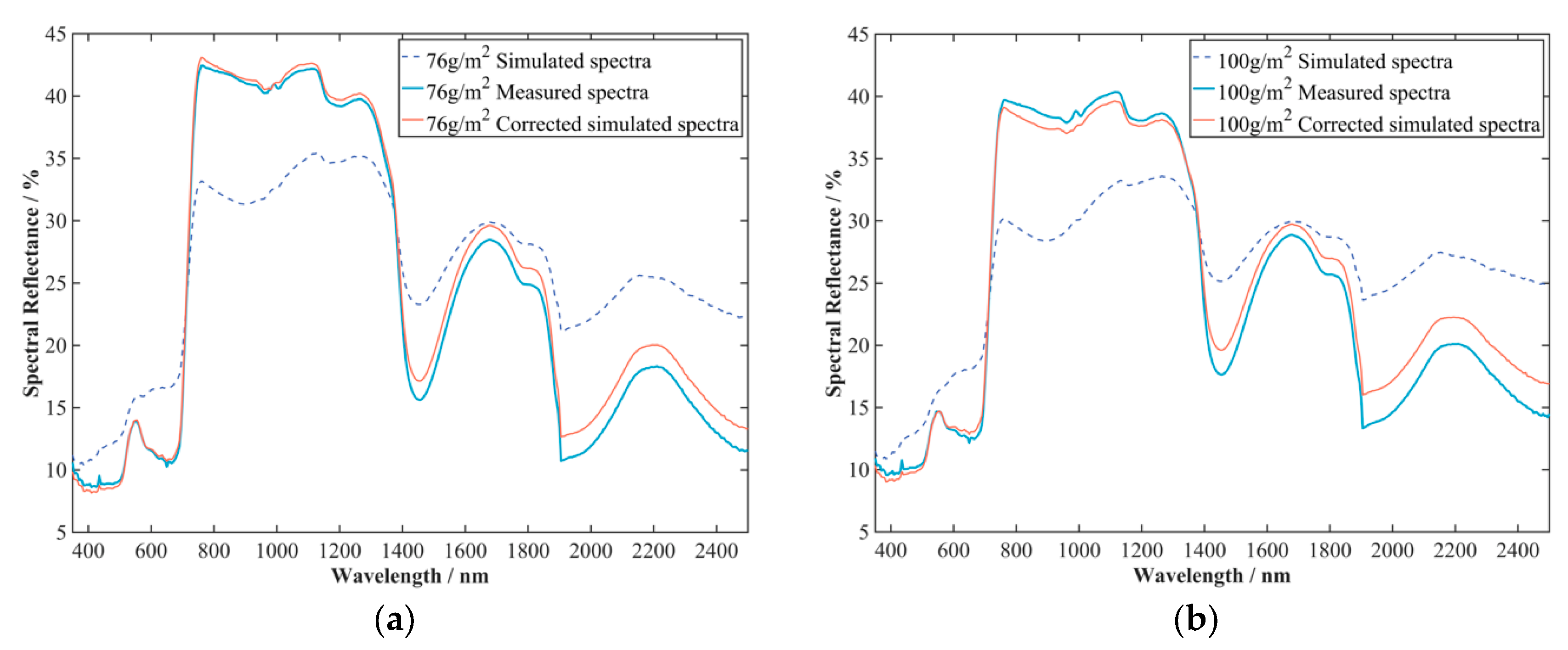
3.2. Results Based on the Fused Model

The simulation spectrum results, after error correction, are shown in Figure 7. For example, the corrected simulated spectra at 76 g/m2 and 100 g/m2 of dustfall are compared to the respective measured spectra and based on the Hapke two-layer medium model simulated spectra as shown in Figure 8. The results show that there is a large difference between the uncorrected curve and the measured curve. When the amount of dustfall is 76 g/m2, the corrected curve is slightly higher than the measured spectral curve. When the amount of dustfall is 100 g/m2 (the number of dust accumulation layers is one), the corrected spectral curve is slightly lower than the measured spectral curve at 710 nm–1400 nm, and slightly higher than the measured curve at 1400 nm–2500 nm.
Taking the amounts of dustfall of 76 g/m2 and 100 g/m2 as examples, Figure 9 shows the difference between the corrected simulated reflectance and the measured value as a function of wavelength, and Figure 10 shows the two-dimensional surface diagram of the difference between the corrected and measured values of the Hapke two-layer medium model simulated spectra. Further analysis of Figure 10 shows that: In the whole band, the difference value does not change greatly with the amount of dustfall; in the range of 720–1370 nm, most of the difference values are negative; and the corrected spectra are smaller than the measured spectra. In the range of 1370 to 2500 nm, the difference is positive as a whole, and the greatest difference is 3.4%, when the amount of dustfall is 200 g/m2.

4. Discussion

In this paper, the spectral correction formula was given for dusty leaves simulated by the Hapke two-layer medium model, based on the dust coverage factor and linear spectral mixing theory. The principle of correcting the formula is as follows: When dust particles are tiled and do not completely cover the leaf area (because the dust is spherical), there are gaps between the particles, and the spectrum of the gaps is the spectrum of the vegetation leaves. The areas covered by dust are calculated as simulated spectral reflectance. It is worth mentioning that a change in coverage is related to the arrangement and accumulation mode of particles: When the accumulation mode changes, the particles may overlap, so the coverage changes accordingly. When the arrangement is different, there is the possibility of sparse or tight arrangement between particles, in which case the dust coverage factor is slightly different. It is clear from the correction, Equation (15), that the dust coverage factor is an important parameter, so it is necessary to explore the impact of dust coverage factor changes on the accuracy of the results in detail. Changes to the dust coverage factor are related to the arrangement and the accumulation mode, leading to changes in the filling factor, which is one of the important parameters of the Hapke two-layer medium model simulation, thus, it is necessary to explore this in detail.

4.1. The Effect of Particle Accumulation on the Filling Factor and the Simulated Spectrum

As mentioned above, different dust particle accumulation modes lead to varying changes in the longitudinal packing density of particles, resulting in larger or smaller gaps between particles. Another sparse arrangement and accumulation mode of dust particles is presented in this paper, as shown in Figure 11.
Based on the assumption of dust particle arrangement and accumulation in Figure 11, the filling factor of particle accumulation, φ , can be easily calculated by Equation (23):
φ = 1 4 3 π d 2 3 d 3 ,
By substituting d = 60 um into the above equation, the filling factor can be calculated, as shown in Equation (24):
φ = 1 π 6 = 0.48 ,
The value of the fractional pore space, p, can be calculated by the following equation:
p = 1 φ ,
The filling factor of 0.48 is greater than the filling factor of 0.35, calculated in Section 2.3.1 above, using the tight arrangement and accumulation method. This is because the interstitial fraction is directly used in the calculation of fractional pore space, p, in the Hapke two-layer medium model, and is therefore affected by the change in the interstitial fraction in the simulation reflectivity calculation of Hapke. A comparison between the results obtained for the above accumulation mode and the final results is shown in Figure 12.

4.2. Calculation and Comparison of the Dust Coverage Factor

Based on the arrangement and stacking shown in Figure 10, the filling factor in this case is 0.48 (as calculated by Equation (23)). The accumulation layer number can be given by Equation (26):
N L = M ( 100 / d ) 2 × m ,
In this case, the equivalent physical thickness is calculated by Equation (27):
t = N L · d ,
The number of dust particles under the corresponding amount of dustfall is given by Equation (28).
N T = N L × ( 100 / d ) 2 ,
In summary, the formula for calculating coverage (linear) can be rewritten as Equation (29):
f d = S c S = N T × π · d 2 2 100 × 100 = π N L 4 ,
When the concept of the dust coverage factor was introduced, it was initially simply calculated in a linear way. Although the error of the result was reduced somewhat, it was still regarded as unacceptable if the error was large. The error surface diagram obtained after introducing the linear coverage is shown in Figure 12.
It can be seen from Figure 12 that the error of the corrected result is somewhat lower than that of the original simulated value, and the maximum difference value is reduced by about 5%. In order to analyze the influence of the different calculation methods of linear coverage and nonlinear coverage on the results, the curve of coverage with the amount of dustfall can be obtained by taking the amount of dustfall as the horizontal coordinate and the dust coverage factor as the vertical coordinate, as shown in Figure 13.
It is clearly observable that in a linear calculation, the linear coverage value is higher than the nonlinear coverage value, in the dust magnitude range of 32 g/m2 to 160 g/m2. Therefore, when the corrected reflectance is calculated according to the correction formula in Section 2.3.2, the Hapke simulation value accounts for more weight. In the band where the simulated value is lower than the measured value, the correction is still not large enough. Based on this situation, the particle stacking method is optimized from linear to nonlinear under the condition that other conditions remain unchanged, and the relation between the number of stacking layers and the coverage is established for error correction. It can be assumed that the error could be further reduced. It is worth mentioning that the nonlinear coverage curve in Figure 13 is also consistent with the measured coverage values in previous studies. The reason for the above phenomenon is that when the coverage increases linearly, before 160 g/m2, the coverage value obtained by the calculation method of linear coverage is higher than that obtained by the nonlinear calculation method. In this instance, when calculating coverage according to the correction formula, the simulated value of Hapke occupies a large weight, and the correction effect is not obvious; the correction curve is still below the measured value. The actual results also confirm the acceptability of the above analysis.
The maximum difference between the correction results calculated based on the above arrangement and accumulation methods, and the measured values, is about 10%, with a large error (as shown in Figure 12). In practice, coverage tends to increase as the magnitude of dust increases. When the particles are fully spread, the dust particles continue to fall into the gaps or accumulate on the particles. Therefore, this is an ideal treatment method that does not fit the actual situation and needs to be further optimized.
If the calculation method of the dust coverage factor is based on the nonlinear increase shown in the formula, since the arrangement of dust particles does not change, the dust magnitude of only one full layer is 88 g/m2. When the magnitude is higher than this value, the coverage also increases accordingly. In this instance, the maximum difference between the corrected result and the measured value is about 6% (as shown in Figure 14), and the error is still large, so it is necessary to consider a more compact arrangement and accumulation, according to Section 2.3, to reduce the error.
If the arrangement and the accumulation of particles in Section 2.3 are used, such an arrangement makes the particles dense, and more dust is required for each full layer. A full layer is on the order of 100 g/m2. In this instance, due to the change in the accumulation mode, when each layer is full but the thickness is insufficient (d + a), the number of layers is one. After exceeding this value, the relationship between the order of magnitude and the number of layers gradually increases until the new layer is full. The maximum difference between the obtained correction result and the measured value was about 3%, which shows that the calculation error was further reduced.

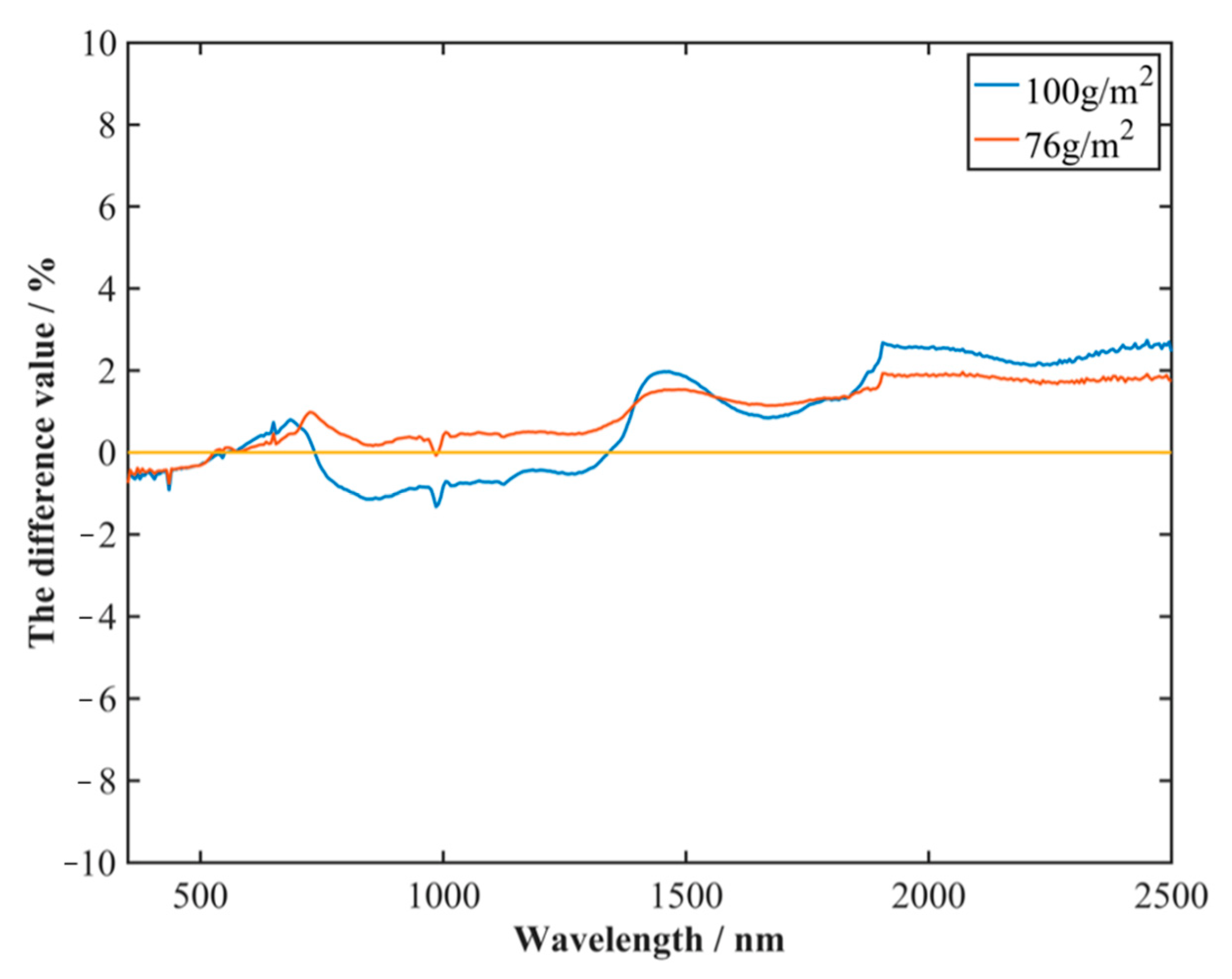
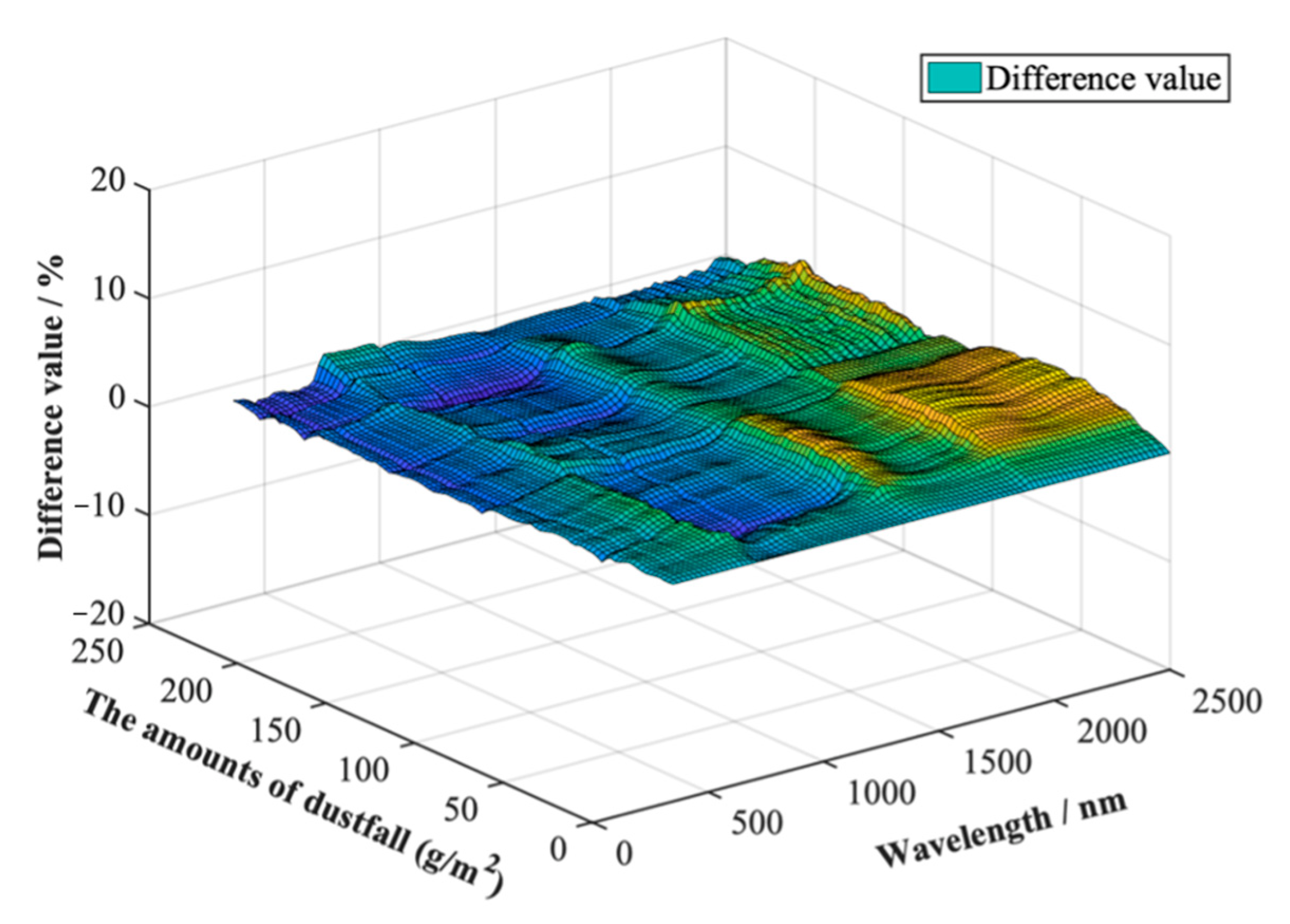
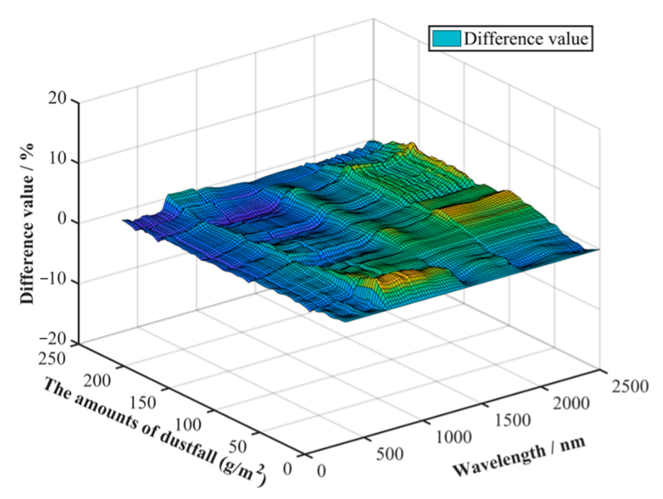
4.3. The Influence of Different Correction Formulas on Error Correction

Because the error correction formula is different, the correction effect is also different; thus, the error correction formula should be analyzed. The error correction formula is given in Section 2.2.2 (Equations (20) and (21)), and is repeated here for completeness.
R = 1 f d × r L + f d × R H a p k e ,
R = 1 f d × r L + f d × R H ,
In this study, Equations (30) and (31) were used to correct the Hapke two-layer medium model simulated spectra. The maximum difference between the corrected spectra and the measured values calculated by the equations was about 3.4%, but the bands were different; the maximum error of Equation (30) occurred in the range of 800–1000 nm (Figure 15), while that of Equation (31) occurred in the range of 2000–2500 nm (Figure 9).

5. Conclusions

The impact of dust pollution on the environment is not negligible. Moreover, rapidly monitoring the magnitude of pollution is an important task. In this study, we used the Hapke two-layer medium model to simulate the leaf spectra of different amounts of dustfall. Due to the limitations of the Hapke two-layer medium model, which cannot accurately simulate the spectra of dusty leaves, the dust coverage factor and the linear spectrum mixing model were used to improve the accuracy. The findings of this study are as follows:
(1) In this paper, the fusing model is proposed. The maximum difference between the simulated spectrum and the measured spectrum with this model is 3.4%, while the maximum difference between the simulated spectrum with the original model is 15.2%. The accuracy of the fusing model is much higher than that of the original model. This overcomes the disadvantage of the Hapke two-layer medium model, that it is inaccurate at smaller amounts of dustfall.
(2) In the Hapke two-layer medium model, the thickness of the upper medium is equivalent, so its calculated simulation spectrum error is large because the dust particles do not completely cover the area of the leaves when the dust amount is small. Therefore, we further optimized the correction formula so that the calculated correction spectrum had higher rationality and reliability.
The method proposed by this study can quickly simulate different amounts of dustfall on leaves’ surfaces, and then quickly invert and calculate dust pollution levels in a mining area, while also providing a convenient and accurate data acquisition method for environmental monitoring in the mining area. The next step regarding this method could be to improve the Hapke two-layer medium model based on wavelength modification: the formulation of a wavelength modification being based on the absorption and reflection characteristics of dust and leaves. In future studies, we will conduct the dustfall experiment with single-size dust particles and mixed-size dust particles, to determine the relationship of the dusty leaf spectra of single-size particles and mixed-size particles. Finally, the dusty leaf spectrum of actual mixed-size dust will be simulated directly.

Author Contributions

Conceptualization, B.M.; data curation, X.Y., Q.L. and M.S.; funding acquisition, D.C. and Y.S.; investigation, B.M., X.Y. and Y.S.; methodology, B.M., D.C. and Q.L.; Resources, B.M., D.C. and Y.S.; software, B.M., X.Y., Y.S., Q.L. and M.S.; supervision, D.C.; writing—original draft, B.M. and X.Y.; writing—review and editing, B.M. and X.Y. All authors have read and agreed to the published version of the manuscript.

Funding

This work was jointly supported by the National Natural Science Foundation of China (41871310 and 41801249), and the Fundamental Research Funds for the Central Universities (N2101006 and N2201007).

Institutional Review Board Statement

Not applicable.

Informed Consent Statement

Not applicable.

Data Availability Statement

The data presented in this study are available upon reasonable request from the corresponding author.

Acknowledgments

We would like to acknowledge the anonymous reviewers for their valuable suggestions.

Conflicts of Interest

The authors declare no conflict of interest.

References

  1. Yan, X.; Shi, W.; Zhao, W.; Luo, N. Mapping dustfall distribution in urban areas using remote sensing and ground spectral data. Sci. Total Environ. 2015, 506, 604–612. [Google Scholar] [CrossRef] [PubMed]
  2. Xu, L.; Mu, G.; Ren, X.; Sun, L.; Lin, Y.; Wan, D. Spatial distribution of dust deposition during dust storms in Cele Oas is, on the southern margin of the Tarim Basin. Arid. Land Res. Manag. 2016, 30, 25–36. [Google Scholar] [CrossRef]
  3. Bali, K.; Mishra, A.K.; Singh, S.; Chandra, S.; Lehahn, Y. Impact of dust storm on phytoplankton bloom over the Arabian Sea: A case study during March 2012. Env. Sci. Pollut. Res. 2019, 26, 11940–11950. [Google Scholar] [CrossRef] [PubMed]
  4. Payne, R.J.; Symeonakis, E. The spatial extent of tephra deposition and environmental impacts from the 1912 Novarupta eruption. Bull. Volcanol. 2012, 74, 2449–2458. [Google Scholar] [CrossRef]
  5. Qi, J.; Nadhir, A.A.; Knutsson, S. Dust Generation within the Vicinity of Malmberget Mine, Sweden. AMM 2011, 90, 752–759. [Google Scholar] [CrossRef]
  6. Lamare, R.E.; Singh, O.P. Effect of cement dust on soil physico-chemical properties around cement plants in Jaintia Hills, Meghalaya. Environ. Eng. Res. 2019, 25, 409–417. [Google Scholar] [CrossRef]
  7. Deng, Q.; Deng, L.; Miao, Y.; Guo, X.; Li, Y. Particle deposition in the human lung: Health implications of particulate matter from different sources. Environ. Res. 2019, 169, 237–245. [Google Scholar] [CrossRef]
  8. Hariram, M.; Sahu, R.; Elumalai, S.P. Impact Assessment of Atmospheric Dust on Foliage Pigments and Pollution Resistances of Plants Grown Nearby Coal Based Thermal Power Plants. Arch. Environ. Contam. Toxicol. 2017, 74, 56–70. [Google Scholar] [CrossRef]
  9. Navrátil, T.; Hladil, J.; Strnad, L.; Koptíková, L.; Skála, R. Volcanic ash particulate matter from the 2010 Eyjafjallajökull eruption in dust deposition at Prague, central Europe. Aeolian Res. 2013, 9, 191–202. [Google Scholar] [CrossRef]
  10. Mandal, K.; Kumar, A.; Tripathi, N.; Singh, R.S.; Chaulya, S.K.; Mishra, P.K.; Bandyopadhyay, L.K.; Council of Scientific and Industrial Research. Characterization of different road dusts in opencast coal mining areas of India. Environ. Monit. Assess 2011, 184, 3427–3441. [Google Scholar] [CrossRef]
  11. Gil-Loaiza, J.; Field, J.P.; White, S.A.; Csavina, J.; Felix, O.; Betterton, E.A.; Sáez, A.E.; Maier, R.M. Phytoremediation Reduces Dust Emissions from Metal(loid)-Contaminated Mine Tailings. Environ. Sci. Technol. 2018, 52, 5851–5858. [Google Scholar] [CrossRef]
  12. Tian, S.; Liang, T.; Li, K. Fine road dust contamination in a mining area presents a likely air pollution hotspot and threat to human health. Environ. Int. 2019, 128, 201–209. [Google Scholar] [CrossRef]
  13. Adhikari, S.; Jordaan, A.; Beukes, J.P.; Siebert, S.J. Anthropogenic Sources Dominate Foliar Chromium Dust Deposition in a Mi ning-Based Urban Region of South Africa. Int. J. Env. Res. Public Health 2022, 19, 2072. [Google Scholar] [CrossRef]
  14. Liu, Y.; Wu, J.; Yu, D.; Ma, Q. The relationship between urban form and air pollution depends on seasonality and city size. Env. Sci. Pollut. Res. Int. 2018, 25, 15554–15567. [Google Scholar] [CrossRef]
  15. Lu, Y.; Wang, Y.; Zuo, J.; Jiang, H.; Huang, D.; Rameezdeen, R. Characteristics of public concern on haze in China and its relationship with air quality in urban areas. Sci. Total Environ. 2018, 637, 1597–1606. [Google Scholar] [CrossRef]
  16. Von Schneidemesser, E.; Steinmar, K.; Weatherhead, E.C.; Bonn, B.; Gerwig, H.; Quedenau, J. Air pollution at human scales in an urban environment: Impact of local environment and vehicles on particle number concentrations. Sci. Total Environ. 2019, 688, 691–700. [Google Scholar] [CrossRef]
  17. Chaudhary, I.J.; Rathore, D. Dust pollution: Its removal and effect on foliage physiology of urban trees. Sustain. Cities Soc. 2019, 51, 101696. [Google Scholar] [CrossRef]
  18. Javanmard, Z.; Kouchaksaraei, M.T.; Hosseini, S.M.; Pandey, A.K. Assessment of anticipated performance index of some deciduous plant species under dust air pollution. Env. Sci. Pollut. Res. 2020, 27, 38987–38994. [Google Scholar] [CrossRef]
  19. Sun, H.; Li, A.; Wu, J. Entrained air by particle plume: Comparison between theoretical derivation and numerical analysis. Part. Sci. Technol. 2019, 39, 141–149. [Google Scholar] [CrossRef]
  20. Cleaver, A.E.; White, H.P.; Rickwood, C.J.; Jamieson, H.E.; Huntsman, P. Field comparison of fugitive tailings dust sampling and monitoring methods. Sci. Total Environ. 2022, 823, 153409. [Google Scholar] [CrossRef]
  21. Watkinson, A.D.; Virgl, J.; Miller, V.S.; Naeth, M.A.; Kim, J.; Serben, K.; Shapka, C.; Sinclair, S. Effects of dust deposition from diamond mining on subarctic plant communities and barren-ground caribou forage. J. Environ. Qual. 2021, 50, 990–1003. [Google Scholar] [CrossRef] [PubMed]
  22. Lin, W.; Li, Y.; Du, S.; Zheng, Y.; Gao, J.; Sun, T. Effect of dust deposition on spectrum-based estimation of leaf water content in urban plant. Ecol. Indic. 2019, 104, 41–47. [Google Scholar] [CrossRef]
  23. Zhu, J.; Yu, Q.; Zhu, H.; He, W.; Xu, C.; Liao, J.; Zhu, Q.; Su, K. Response of dust particle pollution and construction of a leaf dust deposition prediction model based on leaf reflection spectrum characteristics. Environ. Sci. Pollut. Res. Int. 2019, 26, 36764–36775. [Google Scholar] [CrossRef]
  24. Zhu, J.; Xu, J.; Cao, Y.; Fu, J.; Li, B.; Sun, G.; Zhang, X.; Xu, C. Leaf reflectance and functional traits as environmental indicators of urban dust deposition. BMC Plant Biol. 2021, 21, 533. [Google Scholar] [CrossRef] [PubMed]
  25. Zhang, X.-X.; Sharratt, B.; Lei, J.-Q.; Wu, C.-L.; Zhang, J.; Zhao, C.; Wang, Z.-F.; Wu, S.-X.; Li, S.-Y.; Liu, L.-Y.; et al. Parameterization schemes on dust deposition in northwest China: Model validation and implications for the global dust cycle. Atmos. Environ. 2019, 209, 1–13. [Google Scholar] [CrossRef]
  26. Dadashi-Roudbari, A.; Ahmadi, M.; Shakiba, A. Seasonal study of dust deposition and fine particles (PM 2.5) in Iran using MERRA-2 data. Iran. J. Geophys. 2020, 13, 43–59. [Google Scholar] [CrossRef]
  27. Kallel, A.; Verhoef, W.; Le Hegarat-Mascle, S.; Ottle, C.; Hubert-Moy, L. Canopy bidirectional reflectance calculation based on Adding method and SAIL formalism: AddingS/AddingSD. Remote Sens. Environ. 2008, 112, 3639–3655. [Google Scholar] [CrossRef]
  28. Zhai, L.; Wan, L.; Sun, D.; Abdalla, A.; Zhu, Y.; Li, X.; He, Y.; Cen, H. Stability evaluation of the PROSPECT model for leaf chlorophyll content retrieval. Int. J. Agric. Biol. Eng. 2021, 14, 189–198. [Google Scholar] [CrossRef]
  29. Jacquemoud, S.; Verhoef, W.; Baret, F.; Bacour, C.; Zarco-Tejada, P.J.; Asner, G.P.; François, C.; Ustin, S.L. PROSPECT+SAIL models: A review of use for vegetation characterization. Remote Sens. Environ. 2009, 113, S56–S66. [Google Scholar] [CrossRef]
  30. Jacquemoud, S.; Verhoef, W.; Baret, F.; Zarco-Tejada, P.J.; Asner, G.P.; Francois, C.; Ustin, S.L. PROSPECT+SAIL: 15 Years of Use for Land Surface Characterization. In Proceedings of the IEEE International Geoscience and Remote Sensing Symposium (IGARSS), Denver, CO, USA, 31 July–4 August 2006; p. 1992. [Google Scholar]
  31. Wang, Y.; Gastellu-Etchegorry, J.-P. Accurate and fast simulation of remote sensing images at top of atmosphere with DART-Lux. Remote Sens. Environ. 2021, 256, 112311. [Google Scholar] [CrossRef]
  32. Gastellu-Etchegorry, J.P.; Martin, E.; Gascon, F.; Belot, A.; Lefevre, M.J.; Boyat, P.; Gentine, P.; Ader, G.; Deschard, J.; Torruella, P.; et al. DART: 3-D model of optical satellite images and radiation budget. In Proceedings of the IEEE International Symposium on Geoscience and Remote Sensing (IGARSS), Toulouse, France, 21–25 July 2003; IEEE: Piscataway, NJ, USA, 2003; pp. 3242–3244. [Google Scholar]
  33. Hapke, B. Bidirectional reflectance spectroscopy: 1. Theory. J. Geophys. Res. 1981, 86, 3039–3054. [Google Scholar] [CrossRef] [Green Version]
  34. Hapke, B. Theory of Reflectance and Emittance Spectroscopy, 2nd ed.; Cambridge University Press: Cambridge, UK, 2012. [Google Scholar]
  35. Ding, A.; Ma, H.; Liang, S.; He, T. Extension of the Hapke model to the spectral domain to characterize soil physical properties. Remote Sens. Environ. 2022, 269, 112843. [Google Scholar] [CrossRef]
  36. Johnson, J.R.; Grundy, W.M.; Lemmon, M.T. Dust deposition at the Mars Pathfinder landing site: Observations and modeling of visible/near-infrared spectra. Icarus 2003, 163, 330–346. [Google Scholar] [CrossRef]
  37. Al-Hasan, A.Y. A new correlation for direct beam solar radiation received by photovoltaic panel with sand dust accumulated on its surface. Sol. Energy 1998, 63, 323–333. [Google Scholar] [CrossRef]
  38. Beattie, N.S.; Moir, R.S.; Chacko, C.; Buffoni, G.; Roberts, S.H.; Pearsall, N.M. Understanding the effects of sand and dust accumulation on photovoltaic modules. Renew. Energy 2012, 48, 448–452. [Google Scholar] [CrossRef] [Green Version]
Figure 1. The main experimental procedure of this study.
Remotesensing 15 01220 g001
Figure 2. Device for measuring the spectrum of dusty leaves in the dust falling experiment. (a) is a photo of the experimental setup. (b) is a leaf covered with a certain amount of dust.
Remotesensing 15 01220 g002
Figure 3. Particle arrangement and accumulation mode: (a) is the arrangement and accumulation of dust particles on the leaves. (b) is a schematic of the calculation of the value of a.
Remotesensing 15 01220 g003
Figure 4. Spectral curves of leaves with different amounts of dustfall.
Remotesensing 15 01220 g004
Figure 5. The Hapke two-layer medium model simulates the spectral curves of leaves with different amounts of dustfall, the results were calculated using Equation (6).
Remotesensing 15 01220 g005
Figure 6. The difference between the simulated spectral value and the measured spectrum.
Remotesensing 15 01220 g006
Figure 7. The simulation spectrum results after error correction, and the results were calculated from Equations (21) and (22).
Remotesensing 15 01220 g007
Figure 8. The corrected simulated spectral reflectance was compared with the measured spectrum: (a) is the spectrum at a dustfall amount of 76 g/m2; (b) is the spectrum at a dustfall amount of 100 g/m2.
Remotesensing 15 01220 g008
Figure 9. The difference curve between the corrected simulated and the measured values.
Remotesensing 15 01220 g009
Figure 10. Two-dimensional surface diagram of the difference between the corrected and measured values of the Hapke two-layer medium model simulated spectra.
Remotesensing 15 01220 g010
Figure 11. Another arrangement and accumulation mode of dust particles.
Remotesensing 15 01220 g011
Figure 12. Error surface obtained based on the dust accumulation mode shown in Figure 11.
Remotesensing 15 01220 g012
Figure 13. The coverage of linear and nonlinear computation with the amounts of dustfall.
Remotesensing 15 01220 g013
Figure 14. The difference between the corrected results and the measured values.
Remotesensing 15 01220 g014
Figure 15. The variation of the difference between the corrected spectrum and the measured value as a function of wavelength and dust magnitude is calculated by Equation (30).
Remotesensing 15 01220 g015
Table 1. Composition and content of iron tailings dust.
CompositionSiO2TFeFeOMgOAl2O3CaO
Content (%)82.289.901.620.850.730.66
Disclaimer/Publisher’s Note: The statements, opinions and data contained in all publications are solely those of the individual author(s) and contributor(s) and not of MDPI and/or the editor(s). MDPI and/or the editor(s) disclaim responsibility for any injury to people or property resulting from any ideas, methods, instructions or products referred to in the content.

