Random Forest Classification of Multitemporal Landsat 8 Spectral Data and Phenology Metrics for Land Cover Mapping in the Sonoran and Mojave Deserts

Abstract

Geospatial data and tools evolve as new technologies are developed and landscape change occurs over time. As a result, these data may become outdated and inadequate for supporting critical habitat-related work across the international boundary in the Sonoran and Mojave Deserts Bird Conservation Region (BCR 33) due to the area’s complex vegetation communities and the discontinuity in data availability across the United States (US) and Mexico (MX) border. This research aimed to produce the first 30 m continuous land cover map of BCR 33 by prototyping new methods for desert vegetation classification using the Random Forest (RF) machine learning (ML) method. The developed RF classification model utilized multitemporal Landsat 8 Operational Land Imager spectral and vegetation index data from the period of 2013–2020, and phenology metrics tailored to capture the unique growing seasons of desert vegetation. Our RF model achieved an overall classification F-score of 0.80 and an overall accuracy of 91.68%. Our results portrayed the vegetation cover at a much finer resolution than existing land cover maps from the US and MX portions of the study area, allowing for the separation and identification of smaller habitat pockets, including riparian communities, which are critically important for desert wildlife and are often misclassified or nonexistent in current maps. This early prototyping effort serves as a proof of concept for the ML and data fusion methods that will be used to generate the final high-resolution land cover map of the entire BCR 33 region.

1. Introduction

Managing species and habitats in the Sonoran and Mojave Deserts Bird Conservation Region (BCR 33) is challenging due to the area’s transboundary coverage of the United States (US) and Mexico (MX). International borders have hindered the efforts of coordinated management within the region primarily due to the lack of continuous resources available between the neighboring countries, including accurate and current land cover maps [1,2].

Monitoring land cover and land use on a local and regional scale is essential to understanding the continuous effects of climate fluctuations, urbanization, species invasion, and habitat fragmentation on wildlife, including Threatened and Endangered species [3,4]. Land cover maps provide conservationists with critical information about habitat characteristics and distributions, allowing them to determine where and when to conduct monitoring and restoration activities in order to have the largest impact [5]. Within BCR 33, accurate vegetation land cover maps play a critical role in planning and implementing ecological monitoring, particularly in light of the remoteness of habitats and the intense climate conditions within the Sonoran and Mojave Deserts [6].

Both deserts are home to a multitude of endemic species, many of which co-exist across the international border in US and MX territories, making it critical that meaningful conservation efforts support wildlife populations on both sides of the border [7]. One species of particular importance within BCR 33 is the Cactus Ferruginous Pygmy-Owl (Glaucidium brasilianum cactorum). Over the past century, declines in Cactus Ferruginous Pygmy-Owl populations have been largely linked to changes in land use and land cover [8]. A 2018 study used remote sensing data from Landsat to quantify woodland fragmentation and the abundance of woody vegetation cover in order to estimate the quality of Cactus Ferruginous Pygmy-Owl habitats in Pima County, Arizona [9]. Findings from this study highlight the additive value of remote sensing data to existing conservation efforts and support the need for a transboundary land cover map in order to adequately understand and monitor wildlife populations that are divided by international borders.

Remote sensing has also been used in conservation for the identification of invasive species. Studies on both sides of the US and MX border have used high-resolution satellite and unmanned aerial vehicle imagery to detect non-native buffelgrass (Pennisetum ciliare) invading sites throughout the Sonoran Desert [10,11]. The methods used by Elkind et al. were driven by a machine learning (ML) algorithm that used the Random Forest (RF) learning method to classify small patches of buffelgrass from spectral, phenological, and topographic data [10]. The incorporation of supporting environmental variables from vegetation land cover maps allowed the researchers to infer relationships between the distribution of buffelgrass and vegetation types within the study area.

Existing regional land cover maps, whether for the US or MX, over-represent the extent of some land cover types and fail to accurately depict the spatial distribution of vegetation on the Earth’s surface [12]. Additionally, maps created in one country often stop at the international border. This creates a discontinuity in coverage, data quality, and ecosystem classification within transboundary regions such as BCR 33, adding to the challenges of cross-border conservation planning and implementation. Finally, though there are existing transboundary land cover maps of BCR 33, these products lack the level of refinement and geographical extent sufficient to provide effective conservation efforts across the entire region.

Sensor data from air-and space-borne remote sensing technologies are the primary input used in land cover classification. Current land cover classification methods typically use a limited collection of remote sensing seasonal images from the spring, summer, and fall months [13]. When using a limited time frame of data for classification, vegetation land cover classes can exhibit similar readings causing confusion between classes when using automated and visual classification methods [5,14]. Several studies have shown that using multitemporal data provides a higher-fidelity dataset that, in turn, yields better classification results [14,15,16,17]. Classification of multitemporal data on a regional scale has still only been applied within a limited monthly or annual time frame primarily due to the computational workload required and the lack of continuous coverage across some study areas.

The use of multitemporal data additionally allows for the generation and incorporation of phenology metrics in vegetation classification. Phenology is the study of periodic vegetation life cycles and their relationship to seasonal and interannual changes in climate [18]. At the landscape level, phenology is an aggregate response of the dominant cover and, as such, could inform classification. The incorporation of phenology metrics in vegetation classification allows for further separation of vegetation classes based on unique seasonal and spectral characteristics of plant canopy and leaves [17]. Many studies have shown that the use of phenology metrics in addition to spectral data can improve the classification of evergreen, deciduous, and coniferous forest ecoregions [14,17]. Van Leeuwen et al. found that remotely sensed phenological signatures and phenometrics were capable of distinguishing unique vegetation community classes across multiple elevation gradients in the Sonoran Desert [19]. These results suggest that the incorporation of phenology metrics in our classification methods could help to better separate and classify vegetation land cover types within the Sonoran and Mojave Deserts BCR.

With the expansion of input data used for classification, ML classification methods have become more popular in remote sensing for automating classification predictions [20]. The RF classification method has become widely used in the field of remote sensing due to its robust capabilities to achieve excellent classification results within a short processing time and with limited sensitivity to noise compared to other streamlined ML classifiers such as Support Vector Machine and Linear Regression [16,20]. Several studies have shown that the RF method is successful in the classification of land cover classes using Landsat remote sensing data and supporting auxiliary data [21,22]. Although considerable advancements have been made in remote sensing, limitations on the accuracy of land cover type discrimination and the quality of large-scale land cover maps remain, primarily due to the discontinuity between data, methods, and workflow design when performing machine-based land cover classification [23,24].

Objectives

In response to these challenges, this research aims to create the first 30 m continuous land cover map within the Sonoran and Mojave Deserts BCR. The final land cover map and data obtained from this research aim to support research, non-governmental, state, tribal, and federal stakeholders involved in current and future conservation efforts in BCR 33. The specific objectives of this research are:

• Train an ML model to classify vegetation land cover using remote sensing spectral data and phenology metrics from 2013 to 2020, over a large subregion of the Sonoran and Mojave Deserts BCR.
• Calibrate, validate, and refine the final ML-derived vegetation map using a collection of openly sourced remote sensing and ground-based ancillary data, images, and limited fieldwork.
• Harmonize a new transboundary classification system by expanding existing land cover mapping resources from the US portion of BCR 33 into MX.

2. Data and Methods

2.1. Study Area

We developed and prototyped the classification algorithm over a subregion of the Sonoran and Mojave Deserts BCR that spans from Phoenix, Arizona, US to Hermosillo, Sonora, MX (Figure 1). The study area covered primarily the Sonoran Desert region of BCR 33 in southwest Arizona and southeast California, down through both sides of the Gulf of California covering northeast Baja California and western Sonora. In total, the study area was just over 188,000 km². Landsat 8 Operational Land Imager (OLI) data of the study area were assessed over time from April 2013 to December 2020.

BCR 33 was designated by the North American Bird Conservation Initiative (NABCI) [25] and covers the entirety of both the Sonoran and Mojave Deserts, as well as some surrounding ecoregions (Figure 1). The Mojave Desert covers southeast California and southern Nevada. Connected to the southern border of the Mojave Desert is the Sonoran Desert, which extends through southern California, southwest Arizona, northeast Baja California, western Sonora, and northern Sinaloa.

Vegetation land cover in the Sonoran and Mojave Deserts is dominated by desert scrub consisting of a mixture of shrubs, cacti, and grasses. Both deserts hold a significant portion of the world’s endemic desert scrubland, xeroriparian communities, and coniferous “sky-islands” ecoregions that are critical avian habitats [6]. These arid deserts are subject to interannual and seasonal climate variability. The Sonoran Desert receives an annual rainfall average of 76 to 500 mm (3–20 in) [26]. Most of the rainfall in this region occurs during the spring and summer monsoon periods, resulting in bimodal growing seasons at low elevations [19]. Unlike the Sonoran Desert, the Mojave Desert receives a majority of its annual rainfall during winter storms [6]. On average, the Mojave Desert receives an annual rainfall of 101 to 229 mm (4–9 in). Summer temperatures in both deserts can reach up to 48 °C (118 °F). Elevations within the study area range between −86 m (−282 ft) and 3632 m (11,916 ft) [27].

2.2. Reference Land Cover Maps

2.2.1. GAP/LANDFIRE National Terrestrial Ecosystems 2011

Ecological systems from the 2011 GAP/LANDFIRE National Terrestrial Ecosystems [28] were used as a reference for the creation of the land cover classification system used in this research. The Gap Analysis Project (GAP) includes land cover classes as described by NatureServe’s Ecological Systems Classification [29] and land use classes described by the National Land Cover Dataset 2011 [13]. GAP land cover data are limited to only the US; accordingly, one of the goals of this work is to expand the land cover classes from GAP into MX as a starting point for mapping vegetation within the Sonoran and Mojave Deserts BCR.

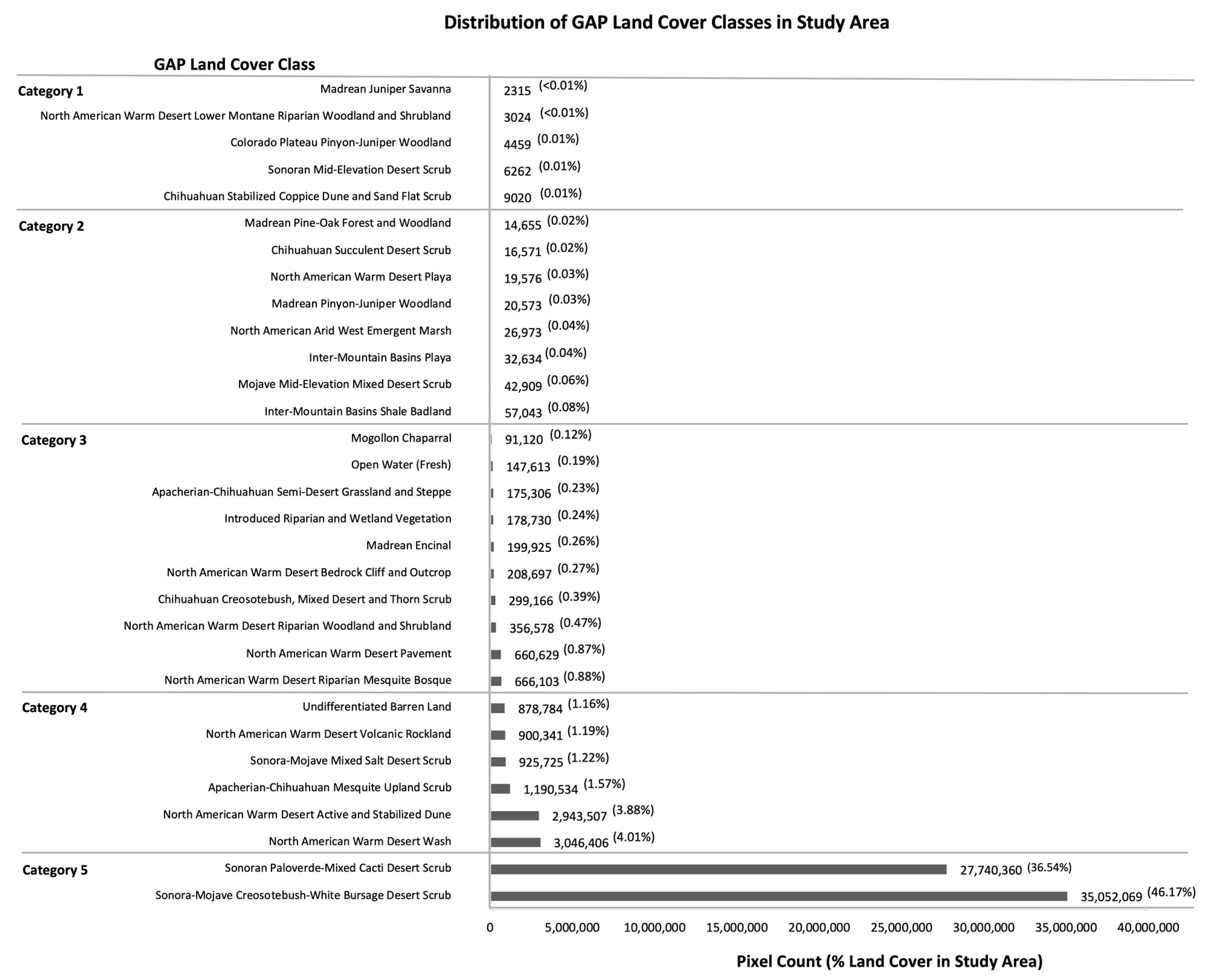
GAP land cover data at 30 m resolution were collected for the US portion of the study area, which was approximately 1/3 of the entire study area (Figure 2). Land cover classes with fewer than 1500 pixels within the study area were not considered in this research, because they did not provide enough training data for the development of the RF classification model. Areas labeled Recently Disturbed or Modified by GAP were also removed given that they have become outdated since their classification in 2011. These classes include recently burned shrubland and forests, recently logged or harvested forests, and disturbed/successional shrub, grass, and forests. Agriculture and developed land cover classes including urban areas, quarries, and mines were not included in the development of the RF model, to reduce confusion between classes. These areas were added from ancillary resources once the final map was complete. A total of 31 land cover classes were considered for this research as shown in Figure 2. Summary reports and descriptions of all GAP land cover classes are available by state at https://doi.org/10.5066/F7ZS2TM0 accessed on 21 July 2021 [28].

2.2.2. INEGI Land Use and Vegetation

Classification results of land cover within the MX region of the study area were validated using data from the Series VII Use of Soil and Vegetation map created by the National Institute of Statistics, Geography, and Informatics (INEGI) [30]. This land use and vegetation map was created using a collection of remotely sensed and ground-based data collected over the past fifteen years. The map classifies vegetation according to the INEGI vegetation classification system [31], which is adapted from two of the most widely accepted vegetation nomenclatures in MX by Rzedowski [32], and Miranda and Hernández X. [33]. This map was chosen as a validation source over other available land cover maps of MX because it documents an array of vegetation types that encompass many of the selected land cover classes used in this research, and INEGI has conducted extensive field trials in the validation of the developed product.

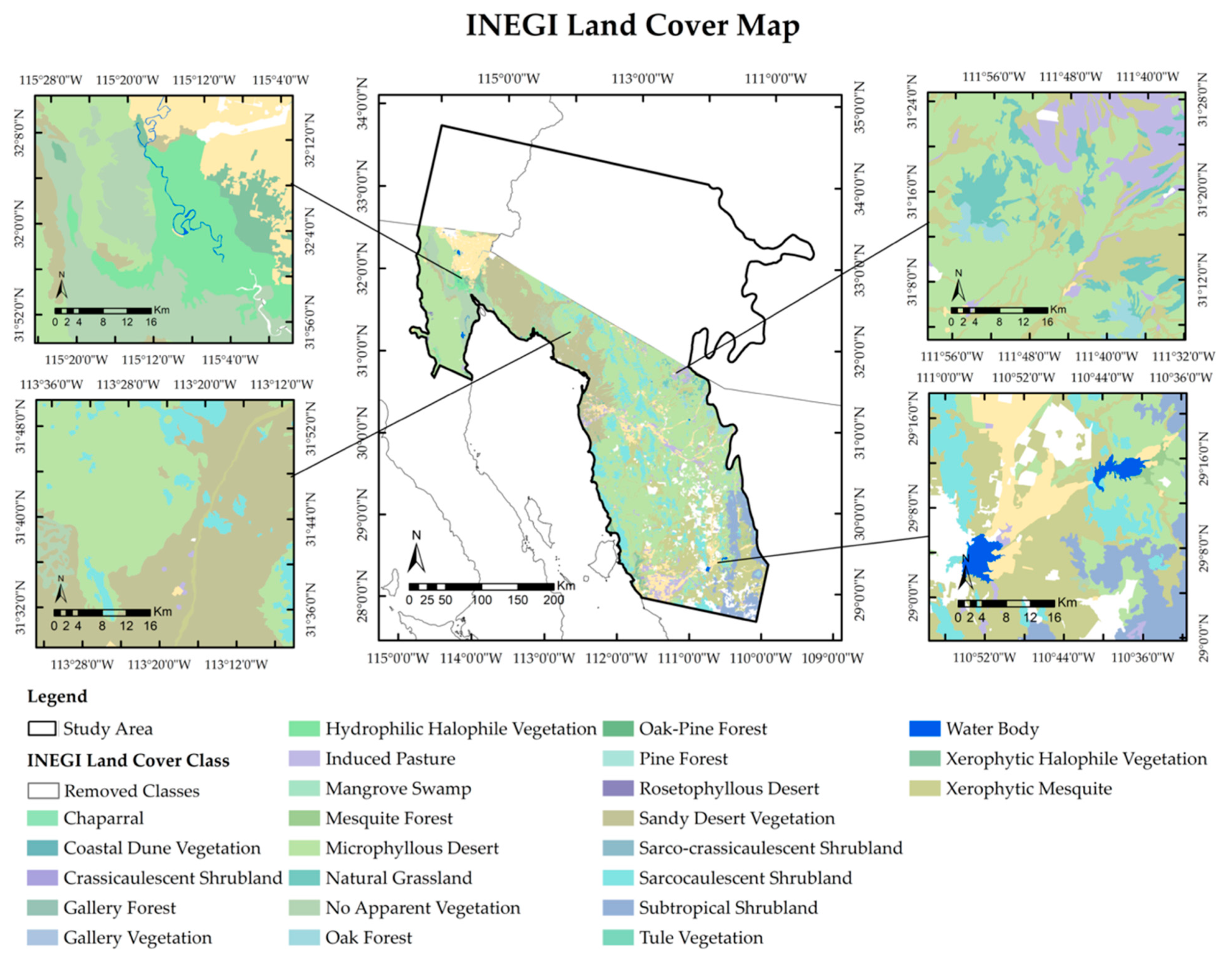
INEGI land use and vegetation classes within the study area were simplified to a final count of 24 classes by merging primary and secondary vegetation classes of the same type and removing classes with less than 1500 pixels within the study area (Figure 3). Areas classified as agriculture or developed land cover classes were visually validated and later added to the final land cover map. The land use and vegetation data can be downloaded as a vector dataset at a scale of 1:250,000 from the INEGI website, https://inegi.org.mx/temas/usosuelo/ accessed on 24 March 2022 [34].

2.2.3. Ancillary Maps

Agricultural land cover was added to the final map using the United States Department of Agriculture (USDA) Cropland Data Layer (CDL) [35,36]. For best practices, the most recent data release based on 2017–2021 cropland data was used for this study. The CDL dataset was validated visually using Google Earth and corrected if areas were misclassified as cropland. This research was not concerned with classifying the type of crop cover, but rather properly isolating cropland areas so that misclassified ecoregions could be fixed. CDL data and supporting documentation can be retrieved from nass.usda.gov/Research_and_Science/Cropland/Release/ accessed on 7 April 2022 [37].

During the correction process of the CDL, it was evident that many wetland and riparian habitats were misclassified as cultivated land. To accurately and efficiently correct these areas, the U.S. Fish and Wildlife Service’s National Wetland Inventory dataset was used to mask and remove wetland and riparian habitat locations [38,39].

2.3. Landsat 8 OLI Data Collection and Processing

Landsat 8 OLI data at 30 m resolution were acquired from the Earth Resources Observation and Science (EROS) Center of the U.S. Geological Survey (USGS) [40]. This research utilized data from the Blue (0.45–0.51 µm), Green (0.53–0.59 µm), Red (0.64–0.67 µm), Near-infrared (NIR) (0.85–0.88 µm), and Short-wave infrared (SWIR1) (1.57–1.65 µm) bands, as well as the Normalized Difference Vegetation Index (NDVI) (Equation (1)). The 2-band Enhanced Vegetation Index (EVI2) was calculated using the NIR (${\mathsf{\rho }}_{\mathrm{NIR}}$) and Red (${\mathsf{\rho }}_{\mathrm{red}}$) bands only as shown in Equation (2) [41]. NDVI and EVI2 complement each other and allow for better separation of vegetation land cover at both ends of the indices’ dynamic ranges [42]. NDVI performs well globally but shows weakness over dense vegetation, and open canopies with different soil backgrounds, with changing soil color and changing atmosphere, while EVI has a more muted dynamic range that performs better over dense vegetation and can better minimize the impact of background and atmospheric effects.

$$\mathrm{NDVI}=\frac{{\mathsf{\rho }}_{\mathrm{NIR}}-{\mathsf{\rho }}_{\mathrm{red}}}{{\mathsf{\rho }}_{\mathrm{NIR}}+{\mathsf{\rho }}_{\mathrm{red}}}$$

(1)

$$\mathrm{EVI}2=2.5\frac{{\mathsf{\rho }}_{\mathrm{NIR}}-{\mathsf{\rho }}_{\mathrm{red}}}{{\mathsf{\rho }}_{\mathrm{NIR}}+2.4{\ast \mathsf{\rho }}_{\mathrm{red}}+1}$$

(2)

A total of thirty-two Landsat scenes covering the entire study area were acquired from April 2013 to December 2020 every 16 days. The collected Landsat data were pre-processed to create a high-fidelity record by removing clouds, heavy aerosols, and other contaminants [42]. The Landsat tiles were then merged and spatially organized into a custom geospatial layout of eight tiles measuring 6193 by 6193 pixels with 30 m resolution. This was performed to optimize storage and analysis of the large study region while still maintaining the original Landsat resolution and Universal Transverse Mercator (UTM) projection. Overlapping boundary pixels between Landsat tiles were resolved by removing “no data” value pixels and retaining the highest quality pixels.

The eight years of Landsat data were then condensed into a long-term annual spectral time series for every month (January–December). The long-term monthly average was used to calculate quarterly (3-month intervals starting in the month of January) statistics for every pixel including the average, minimum, maximum, standard deviation, and change in signal (delta) for every band. These quarterly statistics were used in the training and implementation of the developed ML algorithm, which is further discussed in Section 2.6.

2.4. Extraction of Phenology Metrics

NDVI annual profiles were derived from the long-term average or normal profiles for each pixel. From the NDVI annual profiles, phenology can be quantified to describe growing-season parameters and the vegetation biomass. Averaged NDVI values over time summarize the growing stages of green vegetation and portray the “normal” growing conditions within a region [17]. A modified half-max phenology algorithm was used in this research to characterize phenological events from Landsat NDVI data. The half-max approach suggests that the increase and decrease in greenness are most rapid at a 0.5 threshold, indicating the points of leaf onset and offset [18]. This approach was modified for this research to better capture the phenological development periods of desert vegetation by using a 0.35 threshold [43,44]. Setting a threshold at 0.35 elongates the growing season and was shown to be more accurate in representing vegetation dynamics with protracted slow emerging growing seasons, such as those observed in semi-arid regions [43].

Additional parameters were tuned within the phenology extraction algorithm to filter out regions with significantly low NDVI readings including barren and dune land cover, as well as regions with significantly high NDVI readings such as urban vegetated land cover and cropland. The tuned parameters included the minimum and maximum ranges of NDVI values, errors or noise in the time series, and changes over time, as well as the minimum length of a season, and the presence of more than one growing season, which is key in our study region due to the bimodal precipitation regimes [19,44]. When more than one season was observed for a sample, Season 1 was identified as the dominant season. Results produced from the phenology algorithm quantified the following metrics for every Landsat pixel: start of season (SOS), day of peak (DOP), end of season (EOS), length of season (LOS), green-up rate (GUR), green-down rate (GDR), number of seasons (NOS), maximum NDVI (NDVI_Max), and cumulative NDVI (NDVI_Cum) [45]. Descriptions of these metrics are provided in

Table 1. Description of phenology metrics collected in this study using a modified half-max approach with a threshold of 0.35.

Phenology Metric	Description
Start of season (SOS)	Day of year value identified by a consistent upward trend in NDVI starting at a 0.35 threshold.
Day of peak (DOP)	Day of year value identified by maximum NDVI value.
End of season (EOS)	Day of year value identified by a consistent downward trend in NDVI starting at a 0.35 threshold.
Length of season (LOS)	Number of days between SOS and EOS.
Green-up rate (GUR)	Positive rate of change in NDVI.
Green-down rate (GDR)	Negative rate of change in NDVI.
Number of seasons (NOS)	Number of growing periods within a year (365 days).
Maximum NDVI (NDVIMax)	Maximum NDVI value within the growing season.
Cumulative NDVI (NDVICum)	Sum of NDVI over the entire growing season.

.

2.5. Land Cover Sampling Design

The distribution of land cover classes derived from GAP was considerably imbalanced within the study area (Figure 4). This is a common issue faced in land cover mapping methods using ML because of the naturally imbalanced distribution of land cover on the Earth’s surface [16,46,47,48]. In sampling, the imbalanced distribution of classes creates a bias within the ML model in favor of the majority classes, resulting in a higher misclassification rate of minority classes [49].

To account for the imbalance distribution of our dataset, land cover class pixels were resampled for training. Land cover classes were divided and sampled by categories, similar to the methods produced by Naboureh et al. [46]. Classes were divided into five categories based on their percent land cover within the study area (

Table 2. Sampling categories based on GAP land cover class percent cover in the study area and the evaluated sample fractions for each category.

Category	Land Cover in Study Area (%)	Evaluated Sample Fractions (%)
1	≤0.01	100
2	>0.01 and ≤0.1	40, 60, 80
3	>0.1 and ≤1	4, 6, 8
4	>1 and ≤10	4, 6, 8
5	>10	0.04, 0.06, 0.08

). The number of pixels sampled from each land cover class was then determined by the sampling fraction set by the class’s category.

The sampling fractions applied to each category were chosen based on a trial-and-error approach that took into consideration the size of the land cover classes within each category. The evaluated sampling fractions were selected in intervals of 4, 6, and 8. The magnitude of the sampling fractions varied by category depending on the size of the land cover classes within the category, such that the minority classes in category 1 would be sampled by a larger fraction than majority classes in category 5. This prevented the undersampling of minority classes and the oversampling of majority classes. A total of 81 sampling combinations were evaluated to determine the optimal sampling fraction for each category.

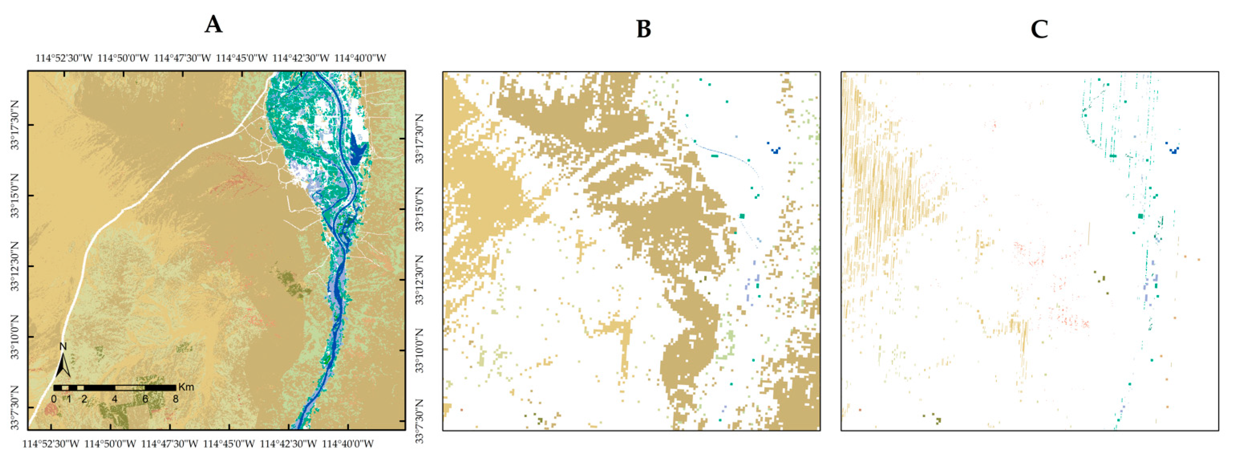
The collected pixel samples for each class were distributed across all eight tiles based on the proportion of class land cover pixels within the tile. Additionally, tile pixel samples were distributed across quadrants within the tiles when possible to capture any variability in the class related to location. Candidates for sampling were selected in clusters of at least a 5 by 5 window (Figure 5B). This ensured that the collected land cover pixels were relatively homogeneous in landcover. For classes that did not have enough clustered pixel samples, additional individual pixels were sampled at random. For classes with more clustered pixel samples than required, pixels were sampled in transects of 50 pixels within the clusters to capture a representative population of homogeneous and mixed boundary pixels (Figure 5C). The locations of the pixel transects were selected at random from within the clusters and distributed across quadrants within the tiles when possible.

Once the optimal sampling fraction was determined for each category, sample sites were visually validated to ensure that the collected samples for training and testing were representative of their assigned land cover class. This process was performed by selecting a sub-portion of sampling sites and visually validating the land cover in those sites using Google Earth Engine [50]. The goal of this exercise was to correct any sampling sites that were visually inaccurate to the observers. When available, the Google Maps Street View feature within Google Earth Engine was utilized to obtain an on-the-ground view of land cover in or near the sample site areas. Any sites that were mislabeled by GAP were corrected and used to retrain the RF model. In total, over 94,000 randomly selected pixels were visually validated across all classes.

2.6. RF Classifier

The RF ensemble learning method [51] was used for pixel-based classification of the long-term quarterly statistics and phenology datasets produced above. RF classification uses an assembly of single decision trees (a forest) to predict a classification output. RF classification was chosen for this research over other ML and deep learning models because of its high-performance capabilities, computational efficiency on large datasets, and effectiveness in classification problems [20].

Development of the RF algorithm was performed in Python (version 3.8, CreateSpace, Scotts Valley, CA, USA) [52]. All processing was run on a Dell Precision 7820 Tower using an Intel ^® Xeon ^® Silver 4110 CPU with dual 2.10 GHz processors, 64 GB RAM, and a 64-bit operating system. The RF classifier algorithm from the Scikit-learn Ensemble Methods Python module [53] was used in the development of the algorithm. Parameter values for the number of trees and number of jobs used in training were modified, with all other parameters set to default values as provided by Scikit-learn. A total of 200 trees were used in training because this value was found to yield the highest classification accuracy in a similar study [24]. To reduce training time, the parameter for the number of jobs was set to −1, indicating the use of all processors in parallel.

Class sample sizes were determined based on the sampling fractions explained earlier in Section 2.5. From the selected pixel samples, 80% were used for training and 20% were retained for testing and validation of the RF model’s performance. Each pixel had a total of 156 features, which included quarterly values for the average, minimum, maximum, standard deviation, and delta of five Landsat 8 OLI surface reflectance bands and two VIs in addition to 16 NDVI phenology metrics, as discussed earlier in Section 2.4.

2.7. Evaluation and Comparison of Classification Results

The most common evaluation metrics used for assessing ML algorithm performance include Overall Accuracy (OA), User Accuracy (UA) (also known as precision), and Producer’s Accuracy (PA) (also known as recall) [47]. Using these metrics to evaluate a model can become problematic when learning using an imbalanced dataset, much like the one used in this study, because the accuracy achieved for each class varies [49]. Thus, evaluating the overall performance of our RF classifier based only on accuracy metrics (OA, UA, and PA) would yield biased results in favor of the majority classes. For this reason, F-score metrics (Equation (3)) [49] were included in the evaluation methods for this research.

$$\mathrm{F}-\mathrm{Score}=2\frac{\mathrm{Precision}·\mathrm{Recall}}{\mathrm{Precision}+\mathrm{Recall}}$$

(3)

Accuracy values were calculated using the Scikit-learn Metrics module [53]. Classification results were further evaluated on a class-by-class basis to observe confusion between classes and determine which classes the model performed the worst on. This was performed using a confusion matrix that compared the predicted classification results to the true classification labels for each land cover type. The final land cover map produced for the entire study area was compared against ancillary mapping data available within the region. A comparison of these maps was performed visually using geospatial applications such as Google Earth Engine [50] and ArcGIS [54].

3. Results

3.1. Sampling Size

The five best performing combinations based on F-score and OA of the 81 evaluated sampling combinations are included in

Table 3. Highest accuracy scores for the evaluated category sampling fraction combinations.

Combination	Sampled Fraction (%)
	Category 1	Category 2	Category 3	Category 4	Category 5	F-Score	OA (%)
22	100	40	6	8	0.04	0.81	91.77
13	100	40	6	6	0.04	0.81	90.78
40	100	40	6	6	0.06	0.81	90.53
67	100	40	6	6	0.08	0.81	90.29
4	100	40	6	4	0.04	0.81	89.81

. Combination 22 using 100% of Category 1, 40% of Category 2, 6% of Category 3, 8% of Category 4, and 0.04% of Category 5 was one of the highest performing combinations in terms of F-score (F-score = 0.81), and the highest in terms of OA (OA = 91.77%). Thus, this combination was used in the development of the final RF model. The worst performing fraction combination used 100% of Category 1, 80% of Category 2, 8% of Category 3, 6% of Category 4, and 0.06% of Category 5 and yielded an F-score of 0.79 and an OA of 88.99%.

3.2. Classification Accuracy

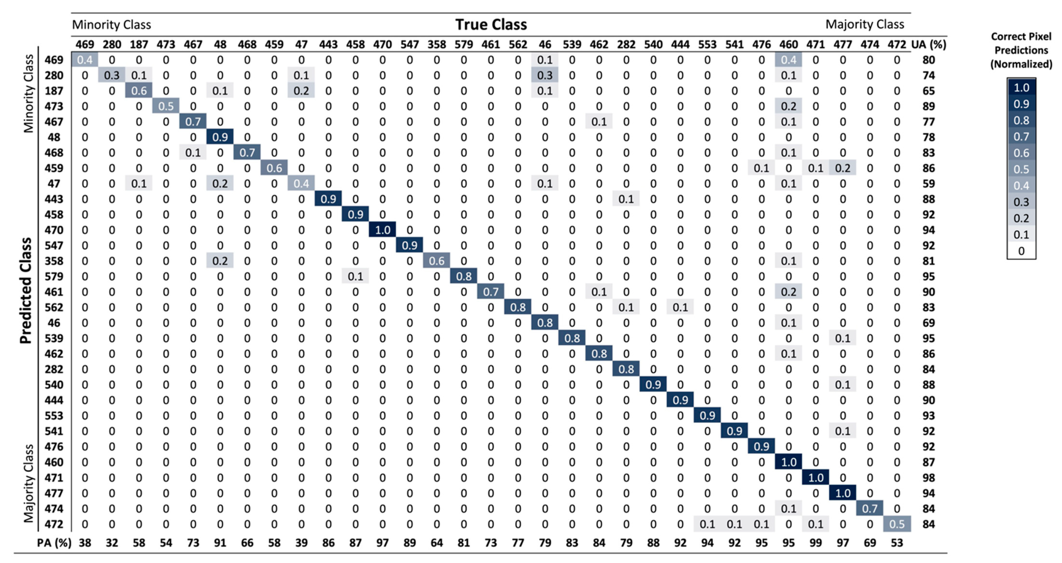
The final model developed used over 80 million pixels for training and achieved an overall F-score of 0.80 and OA of 91.68%, with a total training time just under 5 min. Model accuracy by land cover class is provided below in

Table 4. F-score results for all land cover classes generated from the RF model. These results are obtained from the testing dataset created from labeled GAP data in the US portion of the study area. Top performing classes with an F-score greater than or equal to 0.9 are bolded and the lowest performing classes with an F-score below 0.6 are italicized.

Class Number	Land Cover Class	F-Score
280	North American Warm Desert Lower Montane Riparian Woodland and Shrubland	0.45
47	Madrean Pinyon-Juniper Woodland	0.47
469	Madrean Juniper Savanna	0.52
187	Colorado Plateau Pinyon-Juniper Woodland	0.61
472	Sonora-Mojave Creosotebush-White Bursage Desert Scrub	0.65
473	Sonoran Mid-Elevation Desert Scrub	0.67
459	North American Warm Desert Playa	0.69
358	Mogollon Chaparral	0.72
468	Chihuahuan Succulent Desert Scrub	0.73
46	Madrean Encinal	0.74
467	Chihuahuan Stabilized Coppice Dune and Sand Flat Scrub	0.75
474	Sonoran Paloverde-Mixed Cacti Desert Scrub	0.76
562	Introduced Riparian and Wetland Vegetation	0.80
461	Apacherian-Chihuahuan Semi-Desert Grassland and Steppe	0.81
282	North American Warm Desert Riparian Woodland and Shrubland	0.82
48	Madrean Pine-Oak Forest and Woodland	0.84
462	Chihuahuan Creosotebush, Mixed Desert and Thorn Scrub	0.85
443	North American Arid West Emergent Marsh	0.87
579	Open Water (Fresh)	0.87
540	North American Warm Desert Pavement	0.88
458	Inter-Mountain Basins Playa	0.89
539	North American Warm Desert Bedrock Cliff and Outcrop	0.89
547	Inter-Mountain Basins Shale Badland	0.90
444	North American Warm Desert Riparian Mesquite Bosque	0.91
460	Apacherian-Chihuahuan Mesquite Upland Scrub	0.91
541	North American Warm Desert Volcanic Rockland	0.92
476	Sonora-Mojave Mixed Salt Desert Scrub	0.93
553	Undifferentiated Barren Land	0.94
477	North American Warm Desert Wash	0.95
470	Mojave Mid-Elevation Mixed Desert Scrub	0.96
471	North American Warm Desert Active and Stabilized Dune	0.99

and in the form of a confusion matrix in Figure 6. The minority classes in Category 1 (≤0.01% land cover) were the classes with the most confusion. North American Warm Desert Lower Montane Riparian Woodland and Shrubland was the lowest performing land cover class with an F-score of 0.45, followed by Madrean Pinyon-Juniper Woodland (F-score = 0.47) and Madrean Juniper Savanna (F-score = 0.52). Many of the highest performing classes, with the least confusion, were in Category 4 (>1% and ≤10% land cover), including North American Warm Desert Active and Stabilized Dune (F-score = 0.99), North American Warm Desert Wash (F-score = 0.95), and Undifferentiated Barren Land (F-score = 0.94), as well as Mojave Mid-Elevation Mixed Desert Scrub (F-score = 0.96) from Category 2 (>0.01% and ≤0.1% land cover).

Feature importance values for all 156 features were evaluated using the fitted attribute provided within the Scikit-learn Random Forest Classifier class [53]. The most important features reported from the RF classifier training came from the Blue, EVI2, and SWIR1 bands, as recorded in

Table 5. Highest ranking features in terms of importance to the RF model.

Feature	Statistic	Quarter	Importance (%)
BLUE	Min, Max, Average	2, 3	1.5–1.8
EVI2	Min	3	1.7
SWIR1	Max	2	1.5

. The minimum, maximum, and average values of these bands were the most important statistics. Of these bands, quarters 2 (April–June) and 3 (July–September) were the most important. With respect to phenology metrics, the Season 1 NDVI_MAX value was the most important feature followed by the Season 1 DOP and SOS. All of the Season 2 phenology metrics used in training were the least significant to the model’s predictions.

3.3. Classification of the Entire Study Area

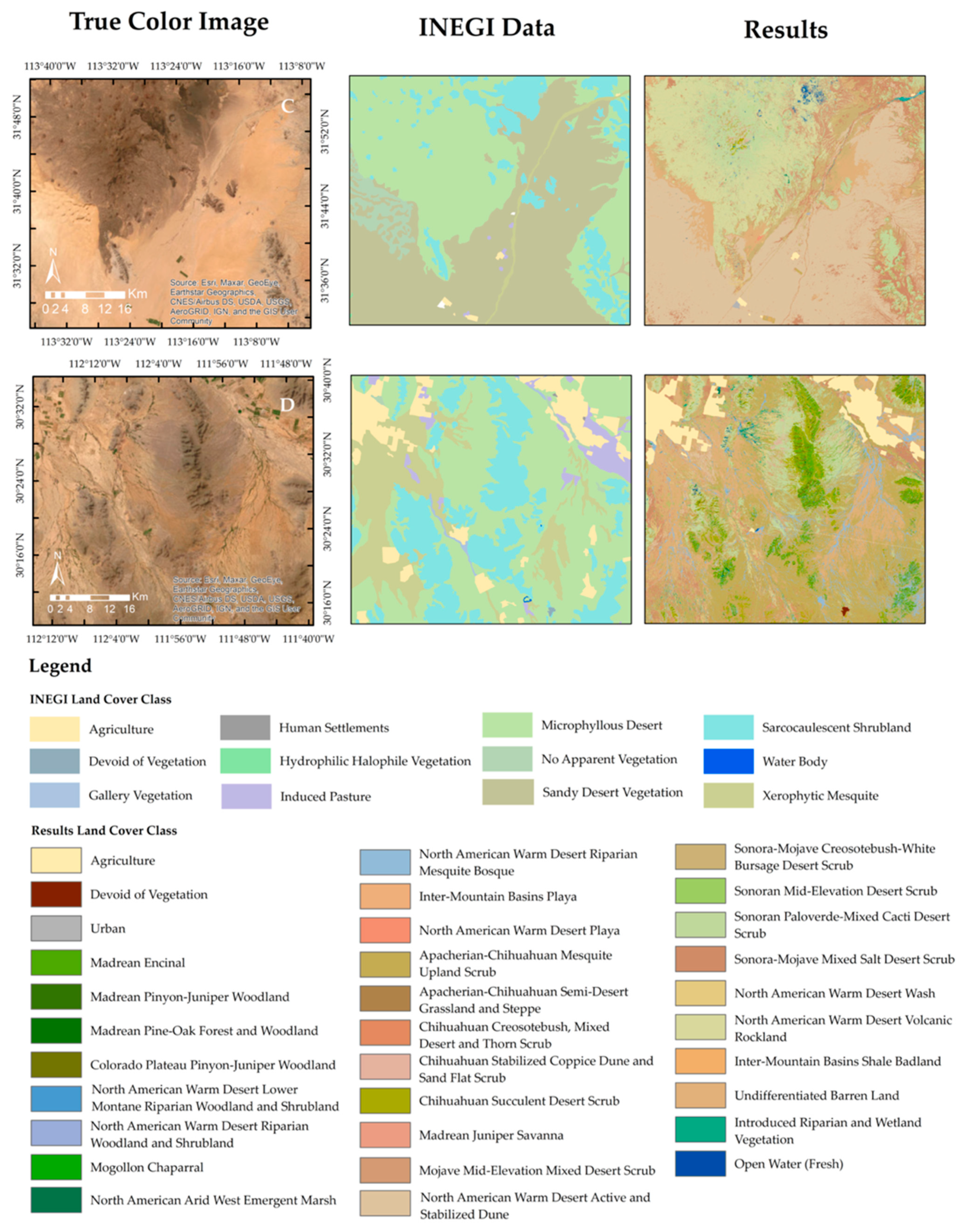
The final land cover map of the entire study area is shown in Figure 7. Subregions of the study area within MX are included in Figure 8, with comparisons of the area’s true color image, INEGI data, and our classification results obtained from the RF model.

3.4. Data Analysis

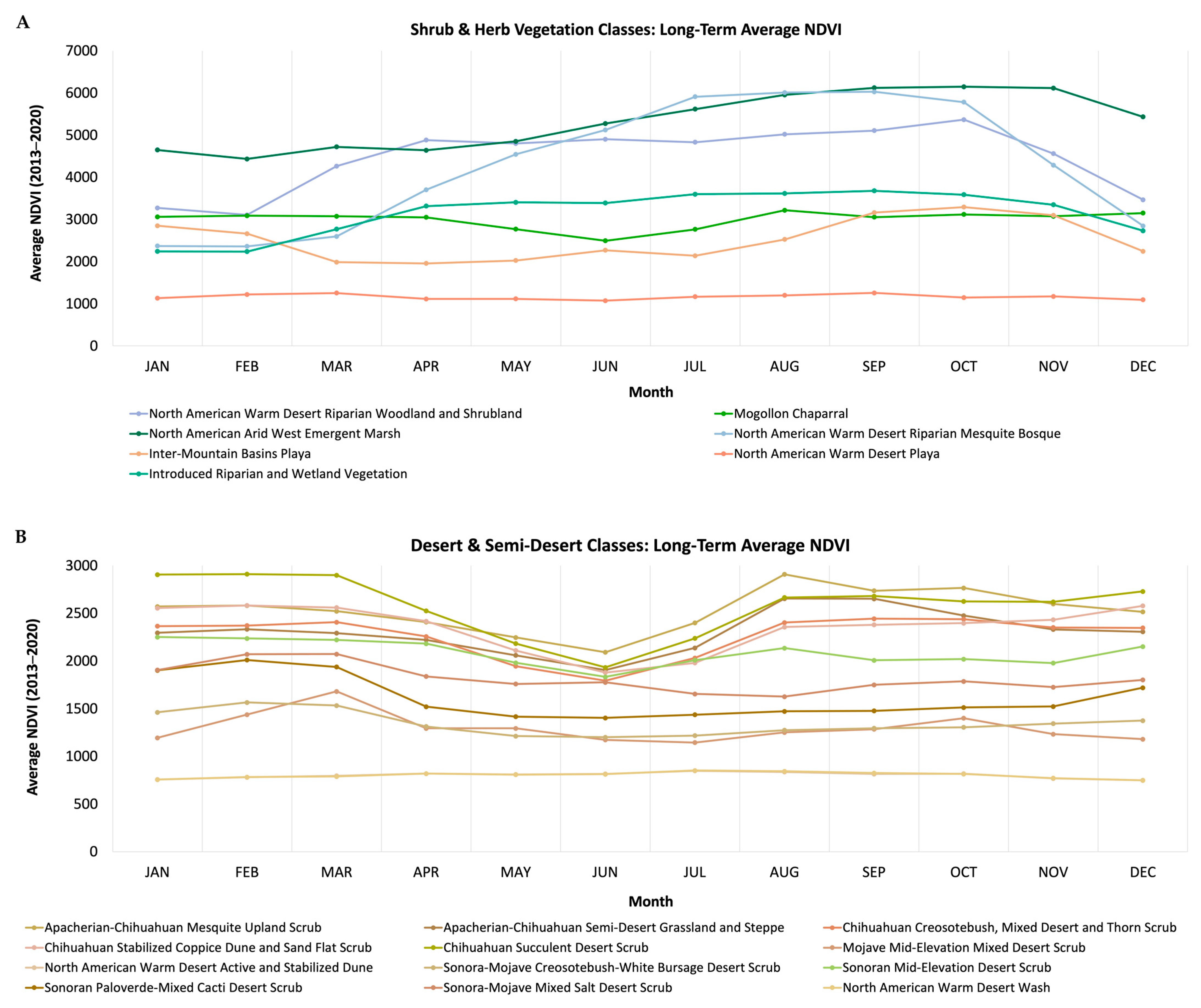
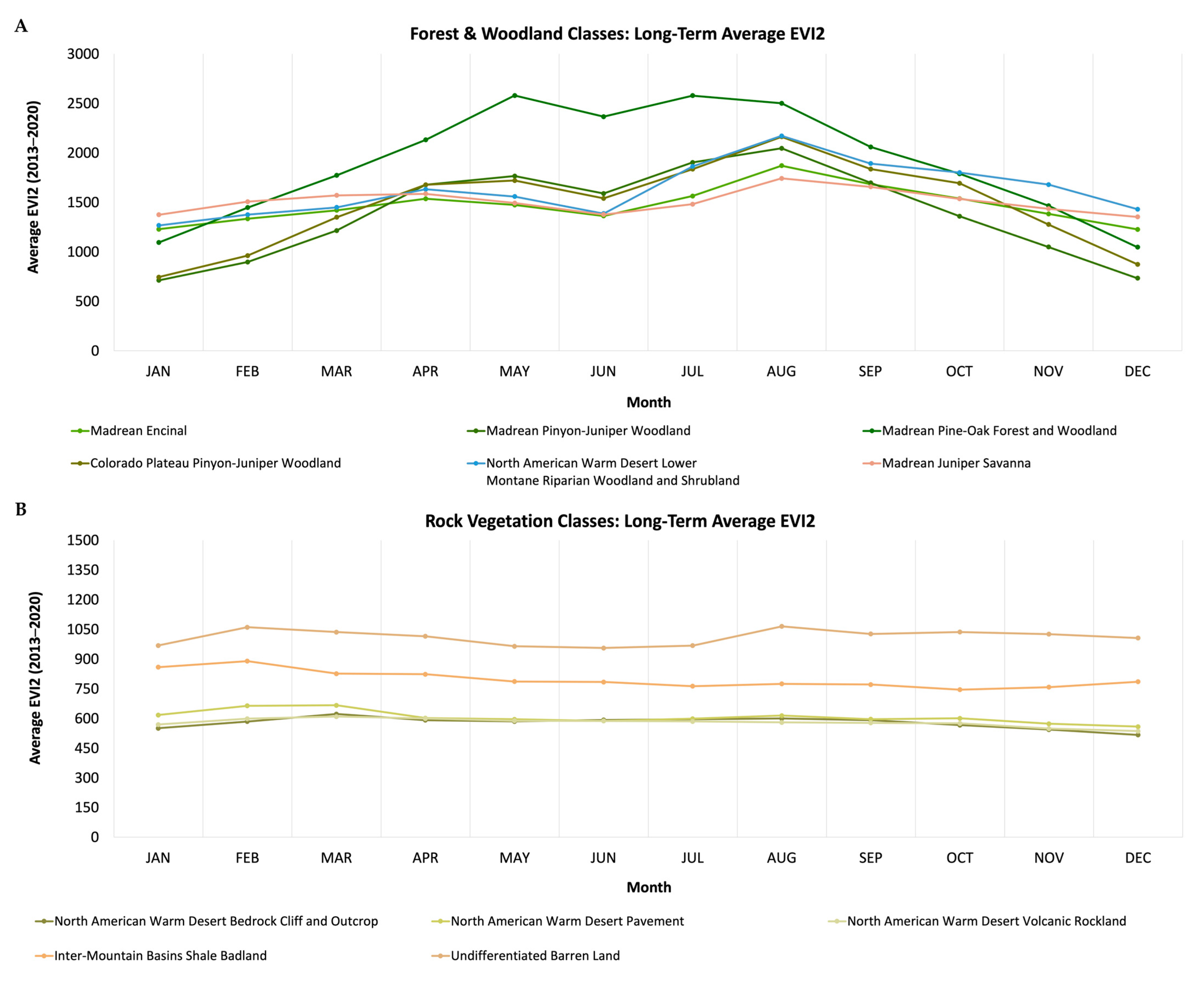
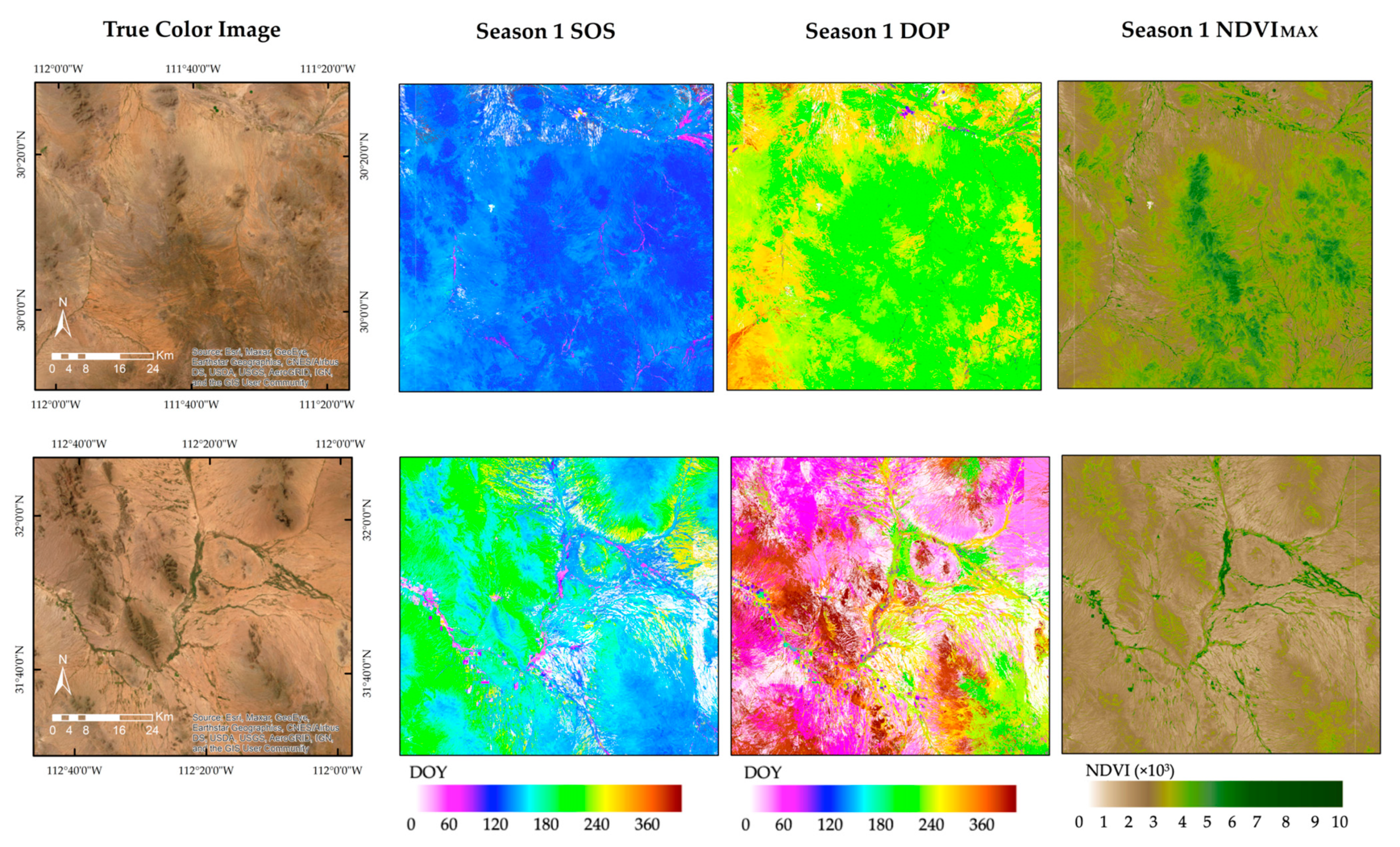
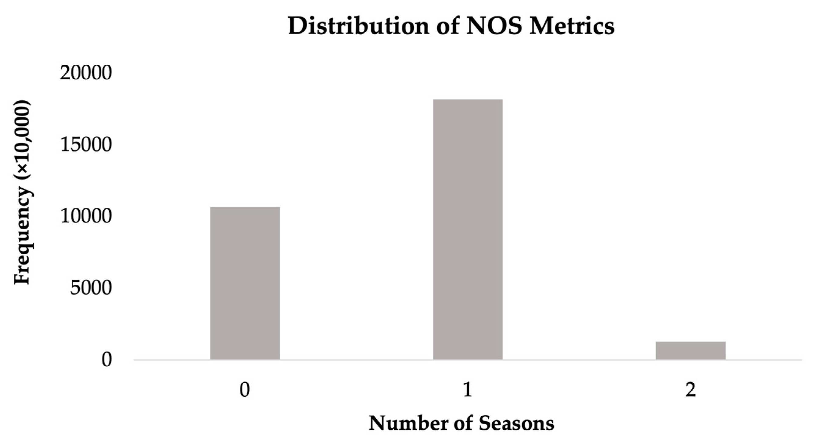
A subset of training pixels from every class was analyzed to observe and compare NDVI and EVI2 long-term average spectral time series by land cover type (Figure 9 and Figure 10). In our study area, EVI2 displayed a smaller dynamic range than NDVI. Both VI time series show an increase in vegetation dynamics during the Spring and Summer months (April–September). Images for the Season 1 SOS, DOP, and NDVI_MAX are displayed in Figure 11, in comparison to the true color image of the sample sites. The distribution of values for the NOS phenology metric was assessed for the entire study area as shown in Figure 12. A majority of the land cover types in our study area displayed only one growing season.

4. Discussions

4.1. RF Model Performance

The variation in accuracies between category sampling combinations was limited but showed that increasing the number of samples from a majority class in category 5, Sonoran Paloverde-Mixed Cacti Desert Scrub and Sonoran-Mojave Creosotebush-White Bursage Desert Scrub, increased confusion among other classes with those classes. To avoid this, the performance of the majority classes was compromised, as seen in the results (Figure 6). Future iterations of this approach could utilize a decomposition-based method that first distinguishes and removes the majority classes and then classifies the remaining classes with a separate algorithm [49].

The model performed best over sparsely vegetated land cover including North American Warm Desert Active and Stabilized Dune (F-score = 0.99), North American Warm Desert Wash (F-score = 0.95), and Undifferentiated Barren Land (F-score = 0.94). These classes covered a large portion of the study area and, thus, provided an adequate number of samples for the training of the RF model. Additionally, these classes represent simpler land cover types that are stable with little change throughout the year, providing for less noise within the signal and consequently more accurate classification (Figure 9B and Figure 10B). The model also performed well on Mojave Mid-Elevation Mixed Desert Scrub land cover (F-score = 0.96). This class appeared to have limited seasonality (Figure 9B) and was found in concentrated regions only within the northwest corner of the study area, which leads into the Mojave Desert.

The model exhibited the greatest confusion on the minority classes in Category 1 (≤0.01% land cover) including North American Warm Desert Lower Montane Riparian Woodland and Shrubland (F-score = 0.45) and Madrean Juniper Savanna (F-score = 0.52). This is likely a result of the limited number of class samples available for use in training the RF model and possible disturbances to the land cover class. These classes, in addition to Madrean Pinyon-Juniper Woodland (F-score = 0.47), are all ecosystems that are commonly found in transitional areas between biomes and are subject to disturbance from external factors such as species invasion and environmental stressors. When averaging spectral signals across the 8 years of data, these disturbances can alter the signal consistency and introduce noise that confuses the classification algorithm further. Improving the model confusion of minority classes is commonly performed by adding additional training samples or improving the quality of existing samples. In land cover mapping, the addition of samples is limited to within a region of interest; thus, oversampling algorithms, such as SMOTE (Synthetic Minority Over-sampling Technique) [55], are commonly used to create synthetic data samples to address this issue [46,47,49].

It is important to note that the feature importance results obtained reflect the model’s decision process and not the data’s scoring. The blue spectral band is often not recognized as an influential band for the assessment of vegetation in remote sensing, due to the short wavelength range and vulnerability to the influence of atmospheric effects, such as aerosols and clouds [41]. Our results suggest that feature data from the blue spectral band improved the separation of land cover classes within our study area, and, in turn, held higher importance in the mode’s classification process. This finding suggests that even though the blue band signal is muted, it nevertheless has a relative value and an ability to separate between classes in this exercise.

EVI2 and NDVI are complementary, as they perform differently when canopy cover density varies [42], and in our study area, EVI2 showed better capabilities at separating land cover types from one another (Figure 9 and Figure 10). This trend is consistent with other studies, which highlighted EVI2′s ability to perform better, considering its ability to remove background soil and residual atmosphere signals. Generally, EVI2 has a smaller dynamic range but better separation capabilities as it responds more to the NIR reflectance, which is more sensitive to vegetation in contrast to NDVI [42,43]. The SWIR band is often used to discriminate between bare soil and vegetation [56] and could have been important to the model’s classification for this reason. Minimum, maximum, and average statistics of these features were considered more important in the model’s classification process because they are unique among all classes, in comparison to standard deviation and delta values, which may become similar amongst classes as they capture a range.

Both quarter 2 (April–June) and quarter 3 (July–September) are times of peak growing activity for vegetation within the Sonoran and Mojave deserts because of the winter moisture followed by the onset of the warm temperatures and monsoon events [57]. In contrast, vegetation is less active during the winter months (quarter 1 (January–March) and quarter 4 (October–December)) when most are in dormancy. This trend was observed in our results (Figure 9 and Figure 10) and can be linked to the increased importance of features from quarters 2 and 3.

Season 2 phenology metrics may have been less important to the model’s decision process because many of the land cover classes within the study area exhibited only one growing season (Figure 12). In addition, Season 1 dominated over season 2 in classes with bimodal growing seasons. Season 1 NDVI_MAX, DOP, and SOS had the highest importance to the model out of all of the phenology metrics used in training (Figure 11). Season 1 NDVI_MAX and DOP illustrate the dynamic ranges of vegetation and are analogous to one another in the indication of vegetation reaching its growth climax. The SOS metric is indicative of vegetation’s ability to initiate growth in response to moisture and annual spring warming and can be different among vegetation types.

4.2. Evaluation of Results in Mexico

Evaluation of the results for the land cover mapping across the US border in MX represented land cover at a much finer resolution than that observed in the INEGI land use and vegetation data (Figure 8). This refinement was noticeable in our evaluations, particularly for the North American Warm Desert Riparian Mesquite Bosque land cover class. This class was in close agreement with INEGI’s Xerophytic Mesquite land cover class. Our results capture the class’s vein-like structure with better definition and extent than the INEGI data, which commonly overrepresented or failed to identify the vegetation type.

It was evident from the INEGI data (Figure 3) that new vegetation types that were not included in our training would appear in the southern region of the study area, particularly along the coast of the Gulf of California. Some of these new vegetation types were considerably different from the vegetation classes used in the training of our RF model, including Mangrove Swamp. This observation gives rise to the need for incorporating additional training classes, such as coastal vegetation, into the model to identify new vegetation types that are unique to the MX region of BCR 33.

5. Conclusions

This research used a set of methods and data fusion approaches using Landsat 8 OLI data and phenology metrics to produce an RF classification model capable of classifying 31 different land cover class types within the Sonoran and Mojave Deserts BCR. The final land cover map produced from this study captured the spatial distribution of vegetation at a much finer resolution than that found in existing land cover maps for both the US and MX. Our results supported the assumption that land cover labels provided within the US portion of the study area were representative of vegetation south of the border, allowing for the extension of the GAP classification system into the MX region of BCR 33. While our results were mostly robust, they did highlight the need for a unified land cover classification scheme across the US and MX portions of BCR 33. Aside from the validation conducted in this study, continuing efforts of this study are focusing on ground-based validation data collection within MX to further assess the accuracy of our results.

An interactive, online data viewing application was prototyped via the University of Arizona Vegetation Index and Phenology Lab website (https://vip.arizona.edu/Borderlands_Project.php accessed on 30 June 2022) to host the final high-resolution land cover map, prepared data, and supporting information obtained through this research. This application serves as a resource to the stakeholders, regional agencies, and non-governmental organizations involved in this research, in support of habitat conservation and land management efforts within the Sonoran and Mojave Deserts BCR.

References

1. Thornton, D.H.; Wirsing, A.J.; Lopez-Gonzalez, C.; Squires, J.R.; Fisher, S.; Larsen, K.W.; Peatt, A.; Scrafford, M.A.; Moen, R.A.; Scully, A.E.; et al. Asymmetric Cross-border Protection of Peripheral Transboundary Species. Conserv. Lett. 2018, 11, e12430. [Google Scholar] [CrossRef] [Green Version]
2. Wehncke, E.V.; Lara-Lara, J.R.; Álvarez-Borrego, S.; Ezcurra, E. Conservation Science in Mexico’s Northwest; Independent Publisher: Chicago, IL, USA, 2014; ISBN 9781495122224. [Google Scholar]
3. Nagendra, H.; Lucas, R.; Honrado, J.P.; Jongman, R.H.G.; Tarantino, C.; Adamo, M.; Mairota, P. Remote Sensing for Conservation Monitoring: Assessing Protected Areas, Habitat Extent, Habitat Condition, Species Diversity, and Threats. Ecol. Indic. 2013, 33, 45–59. [Google Scholar] [CrossRef]
4. Rodríguez-Maturino, A.; Martínez-Guerrero, J.H.; Chairez-Hernández, I.; Pereda-Solis, M.E.; Villarreal-Guerrero, F.; Renteria-Villalobos, M.; Pinedo-Alvarez, A. Mapping Land Cover and Estimating the Grassland Structure in a Priority Area of the Chihuahuan Desert. Land 2017, 6, 70. [Google Scholar] [CrossRef] [Green Version]
5. Horning, N.; Robinson, J.A.; Sterling, E.J.; Turner, W.; Spector, S. Remote Sensing for Ecology and Conservation: A Handbook of Techniques; Oxford University Press: New York, NY, USA, 2010; ISBN 9780199219940. [Google Scholar]
6. (CalPIF) California Partners in Flight. The Desert Bird Conservation Plan: A Strategy for Protecting and Managing Desert Habitats and Associated Birds in California, Version 1.0; California Partners in Flight: Crescent, CA, USA, 2009. [Google Scholar]
7. Martell, A.; Berlanga, H.; Pashley, D.; Hoth, J. Review of Progress on the North American Bird Conservation Initiative; North American Bird Conservation Initiative, NABCI: Gatineau, QC, Canada, 2002. [Google Scholar]
8. Flesch, A.D.; Nagler, P.; Jarchow, C.J.; Richardson, S. Population trends, extinction risk, and conservation guidelines for ferruginous pygmy-owls in the Sonoran Desert. In Final Report for Science Support Partnership Project between U.S. Geological Survey, U.S. Fish and Wildlife Service; Cooperative Agreement No. G15AC00133; University of Arizona, School of Natural Resources and the Environment: Tucson, Arizona, 2017. [Google Scholar]
9. Flesch, A.D. Cactus Ferruginous Pygmy-Owl monitoring and habitat on Pima County Conservation Lands. Report to Pima County Office of Sustainability and Conservation; Contract No. CT-SUS-20-195; University of Arizona, School of Natural Resources and the Environment: Tucson, Arizona, 2021. [Google Scholar]
10. Elkind, K.; Sankey, T.T.; Munson, S.M.; Aslan, C.E. Invasive Buffelgrass Detection Using High-resolution Satellite and UAV Imagery on Google Earth Engine. Remote Sens. Ecol. Conserv. 2019, 5, 318–331. [Google Scholar] [CrossRef]
11. Franklin, K.A.; Lyons, K.; Nagler, P.L.; Lampkin, D.; Glenn, E.P.; Molina-Freaner, F.; Markow, T.; Huete, A.R. Buffelgrass (Pennisetum Ciliare) Land Conversion and Productivity in the Plains of Sonora, Mexico. Biol. Conserv. 2006, 127, 62–71. [Google Scholar] [CrossRef]
12. Pérez-Valladares, C.X.; Velázquez, A.; Moreno-Calles, A.I.; Mas, J.F.; Torres-García, I.; Casas, A.; Rangel-Landa, S.; Blancas, J.; Vallejo, M.; Téllez-Valdés, O. An Expert Knowledge Approach for Mapping Vegetation Cover Based upon Free Access Cartographic Data: The Tehuacan-Cuicatlan Valley, Central Mexico. Biodivers. Conserv. 2019, 28, 1361–1388. [Google Scholar] [CrossRef]
13. Homer, C.; Huang, C.; Yang, L.; Wylie, B.; Coan, M. Development of a 2001 National Land-Cover Database for the United States. Photogramm. Eng. Remote Sens. 2004, 70, 829–840. [Google Scholar] [CrossRef] [Green Version]
14. Knight, J.F.; Lunetta, R.S.; Ediriwickrema, J.; Khorram, S. Regional Scale Land Cover Characterization Using MODIS-NDVI 250 m Multi-Temporal Imagery: A Phenology-Based Approach. GIScience Remote Sens. 2006, 43, 1361–1388. [Google Scholar] [CrossRef]
15. Villarreal, M.L.; Norman, L.M.; Wallace, C.S.A.; van Riper, C., III. A Multitemporal (1979–2009) Land-Use/Land-Cover Dataset of the Binational Santa Cruz Watershed; Open-File Report 2011-1131; U.S. Geological Survey: Reston, VA, USA, 2011; 26p.
16. Shetty, S.; Gupta, P.K.; Belgiu, M.; Srivastav, S.K. Assessing the Effect of Training Sampling Design on the Performance of Machine Learning Classifiers for Land Cover Mapping Using Multi-Temporal Remote Sensing Data and Google Earth Engine. Remote Sens. 2021, 13, 1433. [Google Scholar] [CrossRef]
17. Simonetti, E.; Simonetti, D.; Preatoni, D. Phenology-Based Land Cover Classification Using Landsat 8 Time Series; Publications Office of the European Union: Luxembourg, 2014; ISBN 9789279408441. [Google Scholar]
18. White, M.A.; Thornton, P.E.; Running, S.W. A Continental Phenology Model for Monitoring Vegetation Responses to Interannual Climatic Variability. Glob. Biogeochem. Cycles 1997, 11, 217–234. [Google Scholar] [CrossRef]
19. Van Leeuwen, W.J.D.; Davison, J.E.; Casady, G.M.; Marsh, S.E. Phenological Characterization of Desert Sky Island Vegetation Communities with Remotely Sensed and Climate Time Series Data. Remote Sens. 2010, 2, 388–415. [Google Scholar] [CrossRef] [Green Version]
20. Belgiu, M.; Drăguţ, L. Random Forest in Remote Sensing: A Review of Applications and Future Directions. ISPRS J. Photogramm. Remote Sens. 2016, 114, 24–31. [Google Scholar] [CrossRef]
21. Khatami, R.; Mountrakis, G.; Stehman, S.V. A Meta-Analysis of Remote Sensing Research on Supervised Pixel-Based Land-Cover Image Classification Processes: General Guidelines for Practitioners and Future Research. Remote Sens. Environ. 2016, 177, 89–100. [Google Scholar] [CrossRef] [Green Version]
22. Zhu, Z.; Gallant, A.L.; Woodcock, C.E.; Pengra, B.; Olofsson, P.; Loveland, T.R.; Jin, S.; Dahal, D.; Yang, L.; Auch, R.F. Optimizing Selection of Training and Auxiliary Data for Operational Land Cover Classification for the LCMAP Initiative. ISPRS J. Photogramm. Remote Sens. 2016, 122, 206–221. [Google Scholar] [CrossRef] [Green Version]
23. Gebhardt, S.; Maeda, P.; Wehrmann, T.; Argumedo Espinoza, J.; Schmidt, M. A Proper Land Cover and Forest Type Classification Scheme for Mexico. Int. Arch. Photogramm. Remote Sens. Spat. Inf. Sci. 2015, XL-7W3, 383–390. [Google Scholar] [CrossRef] [Green Version]
24. Li, W.; Dong, R.; Fu, H.; Wang, J.; Yu, L.; Gong, P. Integrating Google Earth Imagery with Landsat Data to Improve 30-m Resolution Land Cover Mapping. Remote Sens. Environ. 2020, 237, 111563. [Google Scholar] [CrossRef]
25. Bird Studies Canada and NABCI. Bird Conservation Regions. Published by Bird Studies Canada on Behalf of the North American Bird Conservation Initiative. 2014. Available online: https://birdscanada.org/bird-science/nabci-bird-conservation-regions (accessed on 5 May 2022).
26. U.S. National Park Service. Sonoran Desert Network Ecosystems. Available online: https://www.nps.gov/im/sodn/ecosystems.htm (accessed on 3 February 2023).
27. U.S. Geological Survey. 3D Elevation Program 1-Meter Resolution Digital Elevation Model. Available online: https://www.usgs.gov/the-national-map-data-delivery (accessed on 1 February 2023).
28. U.S. Geological Survey (USGS) Gap Analysis Project (GAP). GAP/LANDFIRE National Terrestrial Ecosystems 2011; U.S. Geological Survey Data Release: Reston, VA, USA, 2016.
29. Comer, P.D.; Faber-Langendoen, R.; Evans, S.; Gawler, C.; Josse, G.; Kittel, S.; Menard, M.; Pyne, M.; Reid, K. Ecological Systems of the United States: A Working Classification of U.S. Terrestrial Systems; NatureServe: Arlington, VA, USA, 2003. [Google Scholar]
30. National Institute of Statistics, Geography, and Informatics (INEGI). Use of Soil and Vegetation; Serie VII; National Institute of Statistics, Geography, and Informatics (INEGI): Aguascalientes, Mexico, 2018. [Google Scholar]
31. Instituto Nacional de Estadística y Geografía (México). Guía Para la Interpretación de Cartografía: Uso del Suelo y Vegetación: Escala 1:250,000, Serie VI; Instituto Nacional de Estadística y Geografía: Aguascalientes, Mexico, 2017. [Google Scholar]
32. Rzedowski, J.; Huerta, M.L. Vegetación de México, 1st ed.; Editorial Limusa: CDMX, Mexico, 1978. [Google Scholar]
33. Miranda, F.; Hernández-X, E. Los tipos de vegetación de México y su clasificación. Bot. Sci. 2016, 28, 29–179. [Google Scholar] [CrossRef] [Green Version]
34. National Institute of Statistics, Geography, and Informatics (INEGI). Geography and Environment: Use of Soil and Vegetation. INEGI. Available online: https://inegi.org.mx/temas/usosuelo/ (accessed on 24 March 2022).
35. Boryan, C.; Yang, Z.; Mueller, R.; Craig, M. Monitoring US Agriculture: The US Department of Agriculture, National Agricultural Statistics Service, Cropland Data Layer Program. Geocarto Int. 2011, 26, 341–358. [Google Scholar] [CrossRef]
36. United States Department of Agriculture (USDA). National Agricultural Statistics Service 2021 Cropland Data Layer (CDL); United States Department of Agriculture: Washington, DC, USA, 2022. [Google Scholar]
37. United States Department of Agriculture (USDA) National Agricultural Statistics Service. Cropland Data Layer—National Download. Available online: https://www.nass.usda.gov/Research_and_Science/Cropland/Release/ (accessed on 7 April 2022).
38. U.S. Fish and Wildlife Services. Wetlands Mapper Documentation and Instructions Manual; Guidance Document; U. S. Fish and Wildlife Services: Atlanta, GA, USA, 2019.
39. U.S. Fish and Wildlife Services. National Wetlands Inventory Website. Available online: https://www.fws.gov/program/national-wetlands-inventory/wetlands-data (accessed on 9 December 2022).
40. Standart, G.D.; Stulken, K.R.; Zhang, X.; Zong, Z.L. Geospatial Visualization of Global Satellite Images with Vis-EROS. Environ. Model. Softw. 2011, 26, 980–982. [Google Scholar] [CrossRef]
41. Jiang, Z.; Huete, A.; Didan, K.; Miura, T. Development of a Two-Band Enhanced Vegetation Index without a Blue Band. Remote Sens. Environ. 2008, 112, 3833–3845. [Google Scholar] [CrossRef]
42. Huete, A.; Didan, K.; Miura, T.; Rodriguez, E.P.; Gao, X.; Ferreira, L.G. Overview of the Radiometric and Biophysical Performance of the MODIS Vegetation Indices. Remote Sens. Environ. 2002, 83, 195–213. [Google Scholar] [CrossRef]
43. White, M.A.; de Beurs, K.M.; Didan, K.; Inouye, D.W.; Richardson, A.D.; Jensen, O.P.; O’Keefe, J.; Zhang, G.; Nemani, R.R.; van Leeuwen, W.J.D.; et al. Intercomparison, Interpretation, and Assessment of Spring Phenology in North America Estimated from Remote Sensing for 1982–2006. Glob. Chang. Biol. 2009, 15, 2335–2359. [Google Scholar] [CrossRef]
44. Didan, K.; Munoz, A.B.; Miura, T.; Tsend-Ayush, J.; Zhang, X.; Friedl, M.; Gray, J.; Van Leeuwen, W.; Czapla-Myers, J.; Jenkerson, C.; et al. Multi-Sensor Vegetation Index and Phenology Earth Science Data Records Algorithm Theoretical Basis Document and User Guide; NASALP-DAAC: Sioux Falls, SD, USA, 2015. [Google Scholar]
45. Reed, B.C.; Brown, J.F.; VanderZee, D.; Loveland, T.R.; Merchant, J.W.; Ohlen, D.O. Measuring Phenological Variability from Satellite Imagery. J. Veg. Sci. 1994, 5, 703–714. [Google Scholar] [CrossRef]
46. Naboureh, A.; Ebrahimy, H.; Azadbakht, M.; Bian, J.; Amani, M. RUESVMs: An Ensemble Method to Handle the Class Imbalance Problem in Land Cover Mapping Using Google Earth Engine. Remote Sens. 2020, 12, 3484. [Google Scholar] [CrossRef]
47. Douzas, G.; Bacao, F.; Fonseca, J.; Khudinyan, M. Imbalanced Learning in Land Cover Classification: Improving Minority Classes’ Prediction Accuracy Using the Geometric SMOTE Algorithm. Remote Sens. 2019, 11, 3040. [Google Scholar] [CrossRef] [Green Version]
48. McKerrow, A.J.; Davidson, A.; Earnhardt, T.S.; Benson, A.L. Integrating Recent Land Cover Mapping Efforts to Update the National Gap Analysis Program’s Species Habitat Map. Int. Arch. Photogramm. Remote Sens. Spat. Inf. Sci. 2014, XL–1, 245–252. [Google Scholar] [CrossRef] [Green Version]
49. Fernández, A.; García, S.; Galar, M.; Prati, R.C.; Krawczyk, B.; Herrera, F. Learning from Imbalanced Data Sets; Springer International Publishing: Cham, Switzerland, 2018; ISBN 978-3-319-98073-7. [Google Scholar]
50. Gorelick, N.; Hancher, M.; Dixon, M.; Ilyushchenko, S.; Thau, D.; Moore, R. Google Earth Engine: Planetary-Scale Geospatial Analysis for Everyone. Remote Sens. Environ. 2017, 202, 18–27. [Google Scholar] [CrossRef]
51. Breiman, L. Random Forests. Mach. Learn. 2001, 45, 5–32. [Google Scholar] [CrossRef] [Green Version]
52. Van Rossum, G.; Drake, F.L. Python 3 Reference Manual; CreateSpace: Scotts Valley, CA, USA, 2009; ISBN 1-4414-1269-7. [Google Scholar]
53. Pedregosa, F.; Varoquaux, G.; Gramfort, A.; Michel, V.; Thirion, B.; Grisel, O.; Blondel, M.; Prettenhofer, P.; Weiss, R.; Dubourg, V.; et al. Scikit-Learn: Machine Learning in Python. J. Mach. Learn. Res. 2011, 12, 2825–2830. [Google Scholar]
54. ArcGIS Desktop; Esri Inc.: Redlands, CA, USA, 2020.
55. Chawla, N.V.; Bowyer, K.W.; Hall, L.O.; Kegelmeyer, W.P. SMOTE: Synthetic Minority Over-Sampling Technique. J. Artif. Intell. Res. 2002, 16, 321–357. [Google Scholar] [CrossRef]
56. Nguyen, C.T.; Chidthaisong, A.; Kieu Diem, P.; Huo, L.-Z. A Modified Bare Soil Index to Identify Bare Land Features during Agricultural Fallow-Period in Southeast Asia Using Landsat 8. Land 2021, 10, 231. [Google Scholar] [CrossRef]
57. Méndez-Barroso, L.A.; Vivoni, E.R.; Watts, C.J.; Rodríguez, J.C. Seasonal and Interannual Relations between Precipitation, Surface Soil Moisture and Vegetation Dynamics in the North American Monsoon Region. J. Hydrol. 2009, 377, 59–70. [Google Scholar] [CrossRef]
58. Melichar, M.; Didan, K.; Barreto-Muñoz, A.; Duberstein, J.; Nagler, P. Random Forest Classification Data Developed from Multitemporal Landsat 8 Spectral Data and Phenology Metrics for a Subregion in Sonoran and Mojave Deserts, April 2013–December 2020; U.S. Geological Survey Data Release: Reston, VA, USA, 2023.
Figure 1. Bird Conservation Region 33. Sonoran and Mojave Deserts and the study area for this research from Phoenix, Arizona, US to Hermosillo, Sonora, MX.
Remotesensing 15 01266 g001
Figure 2. Footprint of the study area showing the selected GAP land cover classes. A total of 31 classes were selected. Classes that were not considered included land cover classes with fewer than 1500 pixels within the study area, Recently Disturbed or Modified land cover, agriculture land, and urban areas.
Remotesensing 15 01266 g002
Figure 3. INEGI land use and vegetation data within the study area. A total of 24 classes were selected. Removed classes included agriculture and urban areas, which were added at a later time to the final map.
Remotesensing 15 01266 g003
Figure 4. Distribution of population sizes (total number of pixels) within the study area for the selected GAP land cover classes. The land cover classes are ordered in ascending order to show the imbalanced distribution of our dataset. Land cover classes are divided by sampling categories, which are defined in Table 2.
Remotesensing 15 01266 g004
Figure 5. (A) The selected land cover classes from GAP. (B) Clusters created using a 5 by 5 window of land cover class pixels. (C) Selected sampling pixels used in training and testing. The scale bar, north arrow, and grid system shown in Figure 5 (A) applies to all proceeding images.
Remotesensing 15 01266 g005
Figure 6. The final confusion matrix generated from the RF model with an overall F-score of 0.80 and OA of 91.68%. Classes are listed in ascending order based on the number of pixels in each class. Numerical values and gradient color of the cells represent the normalized value of correct pixel predictions. UA (%) scores are included for each class within the last column and PA (%) scores within the last row. Land cover names for each land cover class number can be referenced in Table 4 and total pixel counts for each class can be referenced in Figure 4.
Remotesensing 15 01266 g006
Figure 7. The final transboundary land cover map of the study area classified by the trained RF model. The results shown are classified according to the unified classification system adapted from GAP, which includes agriculture, devoid of vegetation, and urban areas.
Remotesensing 15 01266 g007
Figure 8. Zoomed-in comparisons of true color imagery (left), INEGI data (middle), and results of the RF model (right) within MX regions of the study area. The legends provided represent only the classes shown within the areas. The locations of each area are identified in subregions (C) and (D) of Figure 7. Table S1, provided as Supplemental Material for this publication, shows the comparisons made between classes of the resulting land cover classification system and the INEGI classification system.
Remotesensing 15 01266 g008
Figure 9. Long-term annual average NDVI time series from 2013 to 2020 for (A) shrub and herb vegetation classes and (B) desert and semi-desert classes.
Remotesensing 15 01266 g009
Figure 10. Long-term annual average EVI2 time series from 2013 to 2020 for (A) forest and woodland classes and (B) rock vegetation classes.
Remotesensing 15 01266 g010
Figure 11. Comparison of true color images and Season 1 start of season (SOS), day of peak (DOP), and maximum NDVI (NDVIMAX) for sample sites within the study area. The scale bar, north arrow, and grid system shown in the true color image apply to all proceeding images. In the location shown in the top row, the Season 1 SOS appears to be synchronized around the 120th DOY. The DOP metrics of the area show that even though these vegetation types initiate growth around the same DOY, the rate at which they reach their peak NDVI varies, with some rapidly reaching their peak around DOY 180 and others reaching their peak around DOY 240. The Season 1 NDVIMAX also shows that these vegetation types vary in greenness. In the location shown in the bottom row, much of the vegetation cover has a SOS around the 180th DOY and shows to have a DOP around day 60 of the following year. These areas of land cover also appear to be sparsely vegetated as seen in the Season 1 NDVIMAX metrics.
Remotesensing 15 01266 g011
Figure 12. Distribution of the number of seasons (NOS) metric across all vegetation land cover classes within the study area. A NOS value of 0 indicates areas filtered out with the phenology extraction algorithm, including barren land, urban, and cropland.
Remotesensing 15 01266 g012