1. Introduction
Precipitation is the dominant driver of the earth’s water cycle and provides essential water resources to sustain human life and the earth’s ecosystems. Accurate precipitation information enables more efficient management of water resources and better informs policies confronting climate change. However, measuring precipitation is challenging due to the high precipitation variability and limited measuring capacity. Ground rain gauges and satellites are the traditional sources of precipitation data [
1]. Ground-based precipitation observations are accurate and direct but limited due to sparse and unevenly distributed meteorological stations. In many regions, the distribution of rain gauges is still insufficient. Those regions lack precipitation data to effectively drive hydrologic models that require continuous, high spatial- and temporal-resolution precipitation data. Satellite precipitation products (SPPs) provide a new approach for observing precipitation globally with remote sensing [
2], and play an essential role in modelling hydrology on earth. They have been used extensively in climate change studies [
3].
The visible (VIS), infrared (IR), and microwave (MV) bands are commonly employed in meteorological satellites for the “indirect” measurement of precipitation. The VIS/IR in geosynchronous/geostationary weather satellites primarily produce precipitation estimates based on natural thermal radiation from the cloud top (brightness temperatures). VIS/IR bands are commonly subject to scattering/absorption by the constituent particles of the atmosphere, water molecules, aerosols, water vapour, water droplets, and others. Hence, they are unable to penetrate clouds. In general, the accuracy of estimates based on VIS/IR sensors is relatively low due to the indirect relationship between infrared and precipitation. VIV/IR sensors, however, provide much more frequent coverage thanks to the sensors’ position in geosynchronous orbit. Microwaves (MV), compared to the visible and infrared bands, can penetrate through cloud cover, haze, dust, and all but the heaviest rainfall, as the longer wavelengths are not susceptible to the atmospheric scattering affecting shorter optical wavelengths. This capacity allows the detection of microwave energy under almost all weather and environmental conditions so that data can be collected at any time. Overall, precipitation estimates from VIS/IR are sampled more frequently and have higher resolution but lower accuracy. Precipitation estimates from MV are more accurate but have coarser resolution and less frequent sampling. Precipitation estimates from VIS/IR and MV thus offer complementary features and are often integrated to achieve a better estimate at high temporal and spatial resolution and coverage. Most of the existing satellite precipitation data are, in fact, “blended” products that meld together multiple different “precipitations” from satellite precipitation estimates, existing precipitation grid products, ground rain radar data, and ground rain gauge data. Satellite-blended products perhaps offer a more improved quality than individual datasets [
4].
Multiple satellite-based global (or quasi-global) precipitation products have been developed worldwide during the big data revolution. Many assessment/evaluation/validation studies of SPPs have been conducted by researchers worldwide [
5,
6,
7,
8,
9,
10,
11,
12,
13,
14,
15]. There are eight popular open-sourced SPPs currently: CHIRPS (Climate Hazards Group InfraRed Precipitation with Station data) [
16], CMORPH (Climate Prediction Center Morphing Technique) [
17], GPCP (Global Precipitation Climatology Project) [
18], GSMaP (Global Satellite Mapping of Precipitation) [
19], IMERG (Integrated MultisatellitE Retrievals from GPM) [
20], MSWEP (Multi-Source Weighted-Ensemble Precipitation) [
21], PERSIANN (Precipitation Estimation from Remotely Sensed Information using Artificial Neural Networks) [
22], and SM2RAIN (Soil Moisture TO RAIN) [
23]. Numerous researchers have made a great effort to explore the application potential of those datasets in drought monitoring [
24,
25], catchment hydrologic modelling [
26,
27,
28,
29,
30,
31], extreme precipitation, typhoon and flood disaster monitoring [
32,
33,
34,
35,
36,
37,
38,
39,
40,
41,
42], water resource management in arid and semi-arid regions [
43,
44,
45,
46], and others. While SPPs have demonstrated great potential in catchment water resource management and hydrologic modelling applications, the accuracy of satellite precipitation remains one of the major concerns, repeatedly noted in the above studies and the evaluation/validation studies [
47,
48,
49,
50,
51].
While previous studies may have explored satellite precipitation products in different regions or for different purposes, we specifically address the unique challenges of finding a reliable and continuous satellite precipitation product that can supply long time-series data in the Xiangjiang River basin. This basin is a mountainous catchment situated in the south of China, which is always influenced by rainfall, especially in the “plum” rain season (June–August). Our assessment incorporates different temporal and spatial scales and focuses on the influence of terrain on the accuracy of SPPs. Furthermore, we evaluate the hydrologic performance of SPPs in the long-term simulation of watershed hydrologic processes by coupling SPPs with hydrologic models for this period. This study aims to provide new insights into the comprehensive performance of various SPPs in a typical mountainous catchment. This study should also provide an informative reference for SPP data products for regional applications of satellite precipitation data.
2. Materials and Methods
The assessment involved the following main steps: preparation and pre-processing of the ground-based precipitation observations from the rain gauges and runoff data from the hydrologic stations, acquisition and processing of the mainstream SPPs, evaluation of SPPs from multiple spatio-temporal scales based on the observations from the rain-gauges using a set of performance criteria, evaluation of the terrain influence on the performance of the SPPs in the basin, construction of hydrologic models in the basin, and applicability assessment of SPPs in hydrologic modelling.
2.1. Study Area
The Xiangjiang River basin (24°31′–28°45′N, 110°30′–114°00′E) is a humid basin located in the central-south of China, with an area of 94,660 km
2. The Xiangjiang River, with a total river length of 856 km, is one of the seven major tributaries of the Yangtze River and is located in the middle-upper reaches of the Yangtze River system. The Xiangjiang River basin has a highly rolling topography with elevations ranging from 10 m to 2095 m. The upper reaches are mountainous, while the middle and lower reaches are valley plains, low mountains, and hilly areas (
Figure 1). The Xiangjiang River basin is characterized by a sub-tropical monsoon climate controlled by a southeast monsoon that brings heavy precipitation in summer. From 2007 to 2020, the multi-year average precipitation was 1379 mm, calculated from the interpolated rain gauge observations. The multi-year average reference evapotranspiration (ETo) is approximately 1149 mm, calculated by the Hargreaves-Samani method for the same period. The mean annual runoff depth within the basin (at the outlet of XJRB, Xiangtan station) is 775 mm. Five sub-basins were studied: Guiyang, Hengyang, Hengshan, Zhuzhou, and Xiangtan, with areas of 28,303 km
2, 53,195 km
2, 64,944 km
2, 72,857 km
2, and 82,830 km
2, respectively.
2.2. Dataset Acquisition and Preprocessing
2.2.1. Rain Gauge and Runoff Data
For the evaluation and comparative analysis of the eight satellite precipitation products at grid and watershed scales, we obtained in-situ precipitation and runoff observations from all the rainfall gauges and hydrologic stations. The in-situ precipitation data selected in this study were daily precipitation data (2007–2020) of eleven rain gauges distributed within the basin, provided by the Meteorological Data network (
http://data.cma.cn/en, accessed on 29 April 2021). For the evaluation at the watershed scale, the areal observations used as a reference were generated through the interpolation of gauge observations with the ANUSPLIN techniques [
52,
53]. Despite having only eleven stations within the catchment, we utilized 42 stations from a larger surrounding area to build the precipitation surface for the catchment in order to produce an accurate precipitation surface.
The daily streamflow data of five hydrologic stations (Guiyang, Hengyang, Hengshan, Zhuzhou, and Xiangtan) on the mainstream of Xiangjiang River was sourced from the Hydrology and Water Resources Bureau of Hunan Province, China. The distribution of rainfall gauges and hydrologic stations is shown in
Figure 1.
2.2.2. Satellite Precipitation Products
We selected eight widely used open-source SPPs in this study, including CHIRPS, CMORPH, GPCP, GPM, GSMaP, MSWEP, PERSIANN, and SM2RAIN.
Table 1 summarizes the spatial and temporal coverage, resolution, data source, and reference for the eight products.
CHIRPS (Climate Hazards Group InfraRed Precipitation with Station data) was primarily developed by the USGS Famine Early Warning Systems Network (FEWS NET) and the Climate Hazards Group at the University of California [
16]. It has provided precipitation products with a high spatial resolution of 0.05° from 50°S to 50°N across the world since 1981. The fine spatial resolution and relatively long available recording periods have contributed to the CHIRPS’s widespread attention and use in recent years [
54,
55]. This study evaluates the final CHIRPS product of version 2.0 (hereafter CHIRPS).
CMORPH (Climate Prediction Center Morphing Technique) was published by the Climate Prediction Center (CPC) of the National Oceanic and Atmospheric Administration (NOAA) [
17]. It generates global precipitation products based on PMW and IR with relatively high spatiotemporal resolution (8 km spatial and 0.5-hourly temporal resolution). Research has shown that the gauge-satellite blended CMORPH (CMORPH BLD) improved the original data quality of CMORPH [
56]. In this study, the daily CMORPH BLD (hereafter CMORPH) product derived from the Climate Data Records (CDRs) of the National Oceanic and Atmospheric Administration (NOAA) was evaluated with other satellite precipitation products.
GPCP (Global Precipitation Climatology Project) established by the World Climate Research Program (WCRP), provides 1° daily (and 2.5° monthly) precipitation accumulation from satellite and rain-gauge measurements from 1996 to the present (1979–present for monthly) [
18]. The relatively high resolution and good time continuity of GPCP 1 Degree Daily (1DD) is widely used globally. The dataset of GPCP 1DD (hereafter referred to as GPCP) is included in this study.
GSMaP (Global Satellite Mapping of Precipitation), developed by the JAXA [
19], is a high-resolution global precipitation product produced by the GSMaP project under the (GPM) mission. The algorithm adopts Kalman filtering to estimate the global GSMaP precipitation (with a spatial resolution of 0.1°) hourly with PMW and IR images. The GSMaP used for this evaluation was accumulated from hourly precipitation data using the GEE (Google Earth Engine) platform (including GSMaP Reanalysis and GSMaP Operational products processed by the GSMaP algorithm version 6).
IMERG (Integrated MultisatellitE Retrievals from GPM) precipitation product was developed by NASA in collaboration with JAXA as the successor of NASA’s TMPA (TRMM multi-satellite precipitation analysis) and is another widely used precipitation product of the GPM mission produced with the IMERG algorithm [
20]. The latest IMERG precipitation, IMERG Version 06, released in 2019, reprocessed the TRMM-era with the IMERG algorithm, creating a longer time scale of IMERG precipitation from 2000. The retrospective IMERG precipitation product’s long-term continuous record expands its utility in hydrometeorology research and applications. The IMERG Final Run (hereafter referred to as IMERG), corrected by the Global Precipitation Climatology Centre (GPCC) rain gauge data, provides more accurate estimates and is adopted for comparison in this study.
MSWEP (Multi-Source Weighted-Ensemble Precipitation), developed by Beck et al. [
21], is a long-term global satellite precipitation product with high spatio-temporal resolution [
57]. MSWEP is a historical record for more than 40 years (from 1979 to 2020) and is generated by the anomalous weighted average of a number of precipitation datasets incorporating gauge, satellite, and reanalysis data [
39]. The MSWEP has been updated to Version 2.8 recently with the finest spatio-temporal resolution of 0.1°/3 h. MSWEP V2.8 is generated with two outperforming satellite/reanalysis datasets (ERA5 and IMERG) [
12]. Therefore, the MSWEP V2.8 (hereafter referred to as MSWEP) is selected for the comparative analysis in this study.
PERSIANN (Precipitation Estimation from Remotely Sensed Information using Artificial Neural Networks) was developed by the Center for Hydrometeorology and Remote Sensing (CHRS) at the University of California, Irvine (UCI) [
22]. PERSIANN estimates the precipitation rate based on cloud-top temperature derived from IR images [
58]. PERSIANN CDR (Climate Data Record), with a time delay of 3 months, is a long-term (from 1983-present) daily calibrated product with a relatively high spatial resolution (0.25°) and is usually used for the trend studies of hydrometeorological phenomena. PERSIANN CDR (hereafter referred to as PERSIANN) was employed for the comparative analysis in this study.
SM2RAIN (Soil Moisture TO RAIN) is a newly developed “bottom-up” method estimating precipitation over large areas from soil moisture observations [
23]. Unlike the generating approaches of the other SPPs described above, it avoids estimating the properties of clouds in the “top-down” methods and considers the soil layer as a natural rain gauge. The SM2RAIN-ASCAT is produced jointly by a group of institutions in Europe from the Advanced Scatterometer (ASCAT) satellite soil moisture data through the SM2RAIN algorithm with a spatial resolution of 0.1° (~10 km) on a global scale [
59]. This study includes the daily SM2RAIN-ASCAT (hereafter referred to as SM2RAIN) in the comparative evaluation.
2.3. Methodology
2.3.1. Performance Criteria
Six continuous scores (Spearman’s rank correlation coefficient (CC), Root mean square error (RMSE), Mean Absolute Error (MAE), Bias (BIAS), Relative Bias (R-BIAS), Kling-Gupta efficiency (KGE), and Nash–Sutcliffe efficiency (NSE)) and four categorical scores (Probability of Detection (POD), False Alarm Ratio (FAR), Critical Success Index (CSI), and Heidke Skill Score (HSS)) were selected to provide a comprehensive evaluation of the accuracy and reliability of SPPs. Evaluating precipitation performance uses continuous scores, while the performance of precipitation detection uses categorical scores. The expressions of these metric scores are defined in
Table 2.
The CC is adopted to measure the linear relationship between the rank observed and estimated precipitation, as rainfall is not distributed normally but is heavily skewed. RMSE and MAE are used to characterize the extent of the discrepancy between the observed and estimated precipitation (or runoff), with RMSE more sensitive to large errors. The BIAS and R-BIAS represent the systematic error or general pattern of the estimated precipitation (or runoff) deviating from the observed precipitation (or runoff). The KGE, based on an improved combination of the three diagnostically meaningful components of the mean squared error, has been increasingly used for the comprehensive evaluation of the goodness of fit between estimated precipitation (or runoff model simulations) and observations [
60,
61]. The NSE is a commonly used efficiency metric for evaluating the model’s ability to reproduce the observed data [
62]. The NSE is also calculated on both square-root-transformed and logarithmic-transformed flows (indicated as NSEsq and NSElog), which help to address the sensitivity of the NSE to extreme values in the observed data, particularly in low flow regimes [
63]. These transformations aid in stabilizing the data, allowing the NSE to capture the model efficiency comprehensively. The NSE (or NSEsq/NSElog) is not used for directly evaluating SPPs but is employed in evaluating hydrologic models driven by different SPPs. The categorical scores (POD, FAR, CSI, and HSS) estimate the SPPs’ precipitation detection capability. The POD calculates the proportion of observed precipitation events correctly detected by SPPs. The FAR measures the fraction of non-precipitation events mistakenly identified as precipitation by SPPs. The CSI and HSS are more comprehensive contingency metrics selected to evaluate the SPPs’ ability to identify precipitation events correctly. The CSI takes both probabilities of detection and false alarm rate into account. The HSS measures the overall detection skill accounting for matches due to random chance and can directly reflect the goodness of a product. The threshold for the rain/no-rain classification is set at 1 mm/day in the calculation of categorical scores in order to exclude the impact of extensive drizzles and morning frost or dew. The CC, RMSE, MAE, BIAS, KGE, POD, FAR, CSI, and HSS are used as the evaluation metrics for the SPPs’ accuracy, from grid-gauge to basin scales with precipitation observation (observation interpolation) directly. The KGE, NSE, RMSE, and R-BIAS are used as evaluation metrics for the SPPs’ accuracy in hydrologic modelling. Using multiple performance metrics from various scales and approaches can increase the credibility of the evaluation results and provide a more comprehensive picture of the product’s performance.
2.3.2. Hydrologic Models
The hydrologic model is a critical theoretical basis for quantitatively simulating the characteristics of hydrologic phenomena (e.g., rainfall-runoff) and their process dynamics. This study intends to evaluate the SPPs’ performance in hydrologic modelling through the construction and applicability assessment of hydrologic models driven by each of the various SPPs.
Single models have difficulty depicting the basin’s rainfall-runoff relationship completely. Therefore, an ensemble average of multiple models combining an evaluation of multiple hydrologic models can produce more accurate predictions than a single well-calibrated hydrologic model [
64,
65,
66]. In this study, four well-known hydrologic models, the GR4J model (modèle du Génie Rural à 4 paramètres Journalier) [
67], IHACRES (Identification of Hydrographs and Components from Rainfall, Evaporation and Streamflow data) model [
68], Sacramento model [
69], and HBV model [
70] were selected for the ensemble average assessment of remote-sensing precipitation on hydrologic models in the basin scale.
Appendix A shows the list of parameters of the four rainfall-runoff models used in this study.
The GR4J model is a lumped conceptual rainfall–runoff model with four parameters [
67]. It uses two nonlinear reservoirs for production and sink calculations. The production store controls the storage of rainfall, evapotranspiration, and percolation through the surface soil. The routing of effective rainfall is controlled by the routing store, where quick and slow flows are generated by 10% and 90% of the effective rainfall, respectively [
71].
The IHACRES is a conceptual rainfall–runoff model designed to identify hydrographs and component flows purely from rainfall, evaporation, and runoff data. The IHACRES catchment moisture deficit (CMD) version [
68] is adopted in this study. It consists of two modules: a nonlinear loss module for the generation of effective rainfall, and a linear module for transforming the effective rainfall into a quick flow and a slow flow component.
The Sacramento model is a deterministic, continuous, and nonlinear model. It uses soil moisture accounting to simulate the water balance within the catchment [
69]. The model consists of a two-layer soil structure: an upper surface layer representing interception storage and a lower layer representing groundwater storage. Each layer consists of free (fast components) and tension water storages (slow components).
The HBV model is a semi-distributed model consisting of four routines: the snow routine computes snowmelt and snow accumulation with a degree-day method, the soil routine simulates actual evaporation and groundwater recharge as functions of actual water storage, the response routine computes runoff as a function of water storage, and the routing routine simulates the routing of the runoff to the catchment outlet with a triangular weighting function [
70]. This study uses the HBV-light version with precipitation, potential evapotranspiration, and air temperature as input data [
72].
3. Results
3.1. Evaluation of SPPs at Grid and Watershed Scales
The overall performance statistics were calculated at grid scale (
Figure 2) and watershed scale (
Table 3) in XJRB using daily precipitation from 2007 to 2020.
At the grid scale, a positive BIAS mean is found for CHIRPS, GSMaP, IMERG, and SM2RAIN, and a negative BIAS mean is found for CMORPH, GPCP, MSWEP, and PERSIANN. The GSMaP shows the best performance with the highest mean of CC, KGE, CSI and HSS and the lowest RMSE and MAE among the eight kinds of satellite precipitation products, followed by MSWEP, IMERG, CMORPH, PERSIANN, GPCP, SM2RAIN, and CHIRPS with KGE in descending order. The CHIPRS depicts the highest RMSE and MAE among the eight SPPs. The SM2RAIN shows a high ability in precipitation detection with POD (0.92), while with a big false radio in precipitation detection with FAR (0.57). A more comprehensive assessment of the SM2RAIN’s precipitation detection performance can be obtained through the use of the indices CSI (0.42) and HSS (0.26). Meanwhile, the SM2RAIN shows both a bigger range and an interquartile range for BIAS with a larger BIAS medium when compared with other precipitation products.
At the XJRB watershed scale, a positive bias is found for all the precipitation products. The GSMaP and MSWEP display accurate performance with better CC, KGE, CSI and HSS and lower RMSE and MAE compared to the other six satellite precipitation products. The CMORPH (CC = 0.55), SM2RAIN (CC = 0.6), and IMERG (CC = 0.61) show medium CC (0.55~0.61), and the CHIRPS, GPCP and PERSIANN display a relatively low CC (0.48~0.49) when compared with the gauge interpolated data. The RMSE ranges from 5.41 mm to 9.35 mm with MSWEP, GSMaP, SM2RAIN, IMERG, CMORPH, PERSIANN, GPCP, and CHIRPS in ascending order. The CHIPRS shows the highest RMSE and MAE compared to the other SPPs. Moreover, there is an overall performance enhancement for the eight SPPs at the watershed scale compared with their performance at the grid scale.
3.2. Evaluation of SPPs at an Annual and Seasonal Scale
3.2.1. Evaluation of SPPs at an Annual Scale
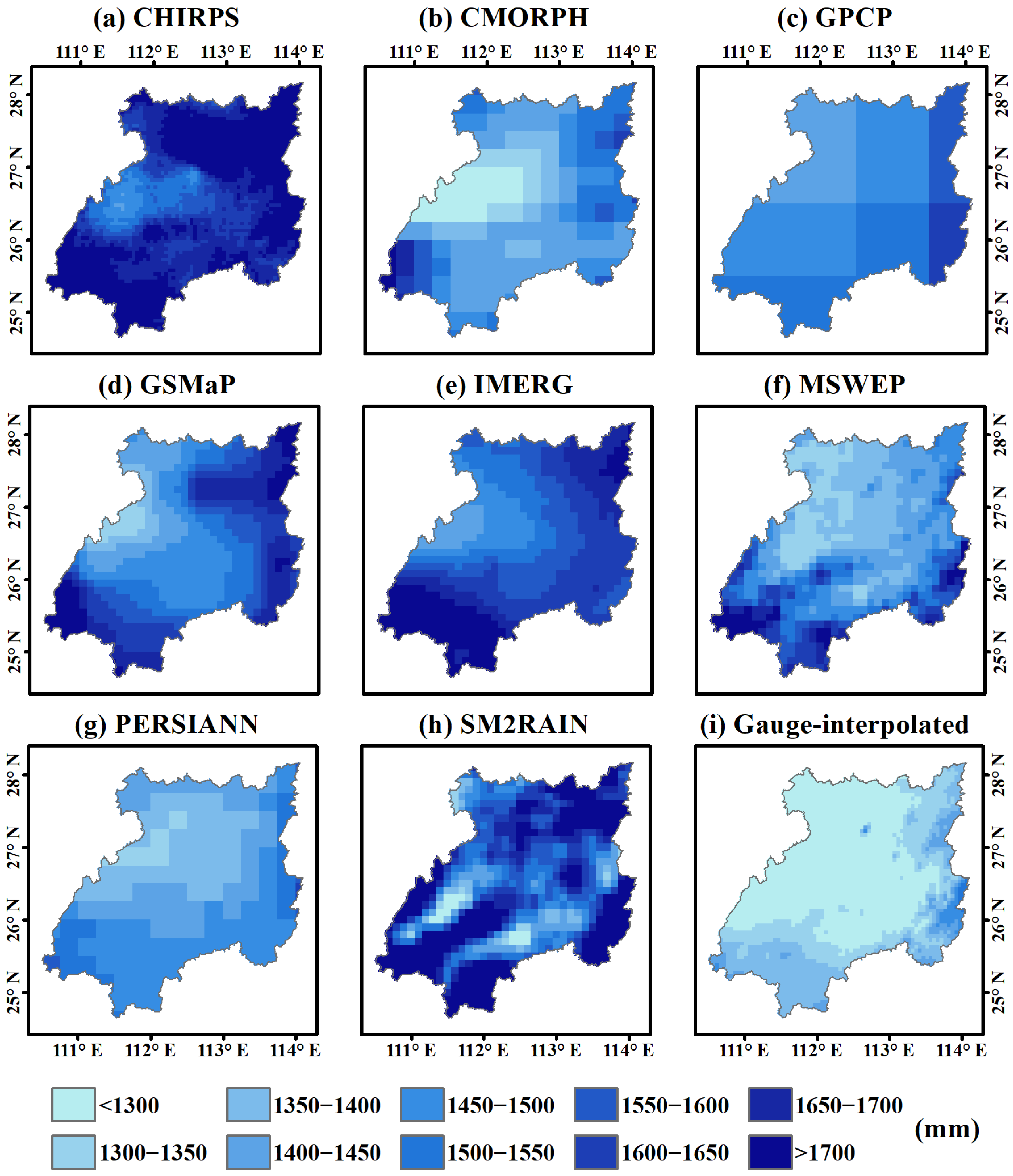
In order to explore the spatial variation of different SPPs, the spatial distribution map of annual average precipitation estimates (
Figure 3) was generated by aggregating and averaging the daily precipitation estimates from 2007 to 2020.
The various precipitation products all show a similar spatial distribution pattern for annual precipitation, with heavy precipitation distributed in the east and south-western regions of the basin and light precipitation distributed in the middle and northern regions of the basin. However, the size of the variation between the various SPPs differs significantly. CHIRPS shows a rainfall centre distributed in the north of the region, which may be a false signal leading to the overestimation of the precipitation distribution in the north of the basin (
Figure 3a). Overall, the SPPs overestimate precipitation annually (from 2007–2020) compared with the interpolation of rain gauge observations. The mean precipitation estimates in ascending order are gauge interpolation (1379 mm), CMORPH (1429 mm), PERSIANN (1431 mm), MSWEP (1472 mm), GPCP (1507 mm), GSMaP (1559 mm), IMERG (1611 mm), SM2RAIN (1670 mm), and CHIRPS (1709 mm).
3.2.2. Evaluation of SPPs at a Seasonal Scale
To assess the accuracy of the eight SPPs in XJRB during different seasons, they were evaluated over the course of four seasons at both the grid scale (
Figure 4) and watershed scale (
Table 4).
At the grid scale, the GSMaP shows the highest CC among the eight satellite precipitation products on a seasonal scale, followed by MSWEP. Compared with GSMaP and MSWEP, the SM2RAIN and IMERG have slightly lower CC. Over the four seasons, the CHIRPS shows the highest RMSE and MAE in Spring (
Figure 4b,c), and other SPPs display a higher RMSE in Summer (
Figure 4b). Among the eight satellite precipitation products, the SM2RAIN displays the biggest overestimate in Spring, while the CMORPH shows the biggest underestimate in Winter (
Figure 4d). Through all four seasons, the GSMaP showed the highest KGE, and the CHIPRS showed the largest fluctuation and instability in its KGE index among the eight SPPs (
Figure 4e). Across the four seasons, the SM2RAIN showed the highest POD and FAR among the eight SPPs (
Figure 4f,g). The CHIRPS shows the smallest POD in Spring, Summer, and Autumn, and the CMORPH shows the lowest POD in Winter among these SPPs (
Figure 4f). Across the four seasons, the GSMaP performs the best with CSI and HSS among the eight SPPs (
Figure 4h,i).
At the watershed scale (
Table 4), the SPPs generally overestimate during the Spring and Summer seasons. The SM2RAIN shows the highest overestimation in Spring, and the CHIRPS shows the highest overestimation in Summer, Autumn, and Winter among the eight SPPs. The CMORPH shows the most considerable underestimation in Winter among these SPPs.
3.3. Evaluation of SPPs by the Distribution of Precipitation Intensity
The frequency distribution (
Figure 5a) and the annual accumulated precipitation distribution (
Figure 5b) for different precipitation intensity classes were generated for a better understanding of the frequency, and the intensity distribution of daily precipitation (from 2007 to 2020) comes from various satellite precipitation products in XJRB. The daily rainfall was divided into four categories (eight classes), namely drizzle (0.1–0.5 mm, 0.5–1 mm), light rain (1–5 mm, 5–10 mm), moderate rain (10–15 mm, 15–20 mm), and heavy rain (20–40 mm and >40 mm).
From
Figure 5a, GSMaP shows a similar frequency distribution to the interpolated gauge data. The IMERG and PERSIANN overestimate the frequency of drizzle (precipitation class 0.1–0.5 mm). The SM2RAIN underestimates the frequency of both drizzle and heavy rain while significantly overestimating the frequency of light rain. From
Figure 5b, the SM2RAIN overestimates the accumulated precipitation of light rain and moderate rain (in the precipitation class of 10–15 mm) and underestimates the accumulated precipitation of heavy rain. The CHIRPS overestimate the accumulated precipitation of heavy rain. The CMORPH and GPCP underestimate the accumulated precipitation of light rain and overestimate the accumulated precipitation of heavy rain. The IMERG overestimated the accumulated precipitation of heavy rain. The GSMaP (in the precipitation class of 20–40 mm) and the PERSIANN (in the precipitation class of >40 mm) also show some overestimation of the accumulated precipitation of heavy rain.
3.4. Evaluation of Terrain Influence on SPPs
The performance of eight SPPs was quantified at different elevations in XJRB to explain how the metrics of the eight precipitation products diverge with increasing elevation (
Figure 6). We observed that, generally, the performance at high elevations is lower than at low elevations. In contrast, the GSMaP shows a relatively stable performance with increasing elevation. As a result, the GSMaP displays good performance, with the highest CC at the rain gauge station at 900 m.a.s.l. elevation and the highest KGE (0.65) at the rain gauge station at 184.9 m.a.s.l. elevation. The CHIRPS performance is poor, with the lowest CC (0.28) calculated at the 900 m.a.s.l rain gauge station and the lowest KGE (0.10) at the rain gauge station at an elevation of 100 m.a.s.l.
Moreover, the RMSE and MAE of all SPPs show a positive relationship with elevation (
Figure 6b,c). The BIAS statistic (
Figure 6d) shows that CHIRPS overestimates the precipitation at all observed altitudes, and SM2RAIN overestimates the precipitation at most elevations. There is an overestimation at lower elevations for GPCP, IMERG, GSMaP, MSWEP, and PERSIANN. The CMORPH underestimated the precipitation across all the observed stations. SM2RAIN at elevation 836 m had the highest positive bias (BIAS = 2.22 mm/day), while the highest negative bias (BIAS = −1.6 mm/day) was found for CMORPH at 900 m elevation.
Overall, the SPPs’ performance (reflected in KGE) decreases with increasing elevation (
Figure 6e). Furthermore, the eight SPPs show a relatively stable performance of POD with a change in altitude. As altitude increases, there is a slight decrease in FAR and a slight increase in CSI for the eight SPPs (
Figure 6g,h). The HSS can detect the declining performance of SM2RAIN with the increase in altitude (
Figure 6i).
3.5. Evaluation of SPPs on Hydrologic Modelling of XJRB
3.5.1. Applicability Assessment of SPPs for Hydrologic Modelling
The performance of the eight SPPs in the rainfall-runoff modelling of XJRB is examined here. The benchmark reference areal precipitation used was from the gauge-observed precipitation and interpolated using ANUSPLIN. The evaluation used four hydrologic models: GR4J, IHACRES, Sacramento, and HBV. The parameter values of the four hydrologic models were calibrated using the shuffled complex evolution algorithm, using 2007–2013 and 2014–2020 as the calibration and validation periods, respectively. The Nash-Sutcliffe efficiency (NSE) was taken as the objective function adopting one year as the warm-up period for calibration. Each model driven by either one of the eight SPPs or gauge-observation interpolation (benchmark) was set up and calibrated with the corresponding precipitation respectively.
Overall, the hydrologic modelling driven by the benchmark performed better compared to hydrologic modelling driven by SPPs. Among the eight SPPs, the hydrologic modelling driven by MSWEP and GSMaP performed the best, followed by IMERG, CMORPH, CHIRPS, GPCP, PERSIANN, and SM2RAIN in a downward trend (
Figure 7a,d,p). The SM2RAIN-driven modelling shows the largest R-BIAS (
Figure 7s). Moreover, the performance of the hydrologic modelling improves as the size of the basin increases (from Guiyang, Hengyang, Hengshan, Zhuzhou, to Xiangtan) (
Figure 7b,e,h,k,n,q,t). Comparing just the hydrologic models (
Figure 7c,f,i,l,o,r,u), all four models performed well with mean KGE > 0.72 and mean NSE > 0.62, with HBV performing the best (KGE = 0.82). The HBV leads in the hydrologic modelling of high, medium, and low flow (NSE = 0.71, NSEsq = 0.68, NSElog = 0.64).
SPP performance during extreme events was assessed during flash flooding in July 2019 (
Figure 8a,c,e,g,i). The best hydrologic modelling performance was shown by the benchmark (interpolated gauge observations), with a high KGE (0.71–0.81) and NSE (0.84–0.90). The GSMaP, IMERG, CMORPH, and CHIRPS performed well also. However, the MSWEP, SM2RAIN, PERSIANN, and GPCP performed relatively poorly compared to the other SPPs. Moreover, these models, especially those driven by the SPPs, tend to underestimate high flow and struggle to predict peak flows in flood events.
The monthly runoff of 2019 (
Figure 8b,d,f,h,j) shows that the hydrologic model driven by the benchmark, IMERG, and CHIRPS performed well, while the SM2RAIN-driven model performed poorly. The SM2RAIN-driven models show heavy overestimation (April–June, September–December), and the GSMaP-driven models show some overestimation (April–June), especially in the middle and lower reaches of XJRB. Overall, the models driven by SM2RAIN and GSMaP have a positive bias (overestimation), while the models driven by GPCP, MSWEP, PERSIANN, CHIRPS, and benchmark have a negative bias (underestimation). The models driven by IMERG and CMORPH overestimate in some basins and underestimate in others.
3.5.2. Evaluating the SPP Influence on Hydrologic Parameters
The calibrated parameters of the four hydrologic models driven by different precipitation products were evaluated, and the results are shown in
Figure 9. For each precipitation product, the optimal parameter value plotted above is the ensemble-averaged parameter value calibrated in five sub-basins of XJRB. Each parameter is normalized to 0–1 min the minimum value of the parameter ranges and then divided by the parameter range.
As input data for a hydrologic model, different satellite precipitation products can bring uncertainties to the model parameters. The parameters X1, X3, and X4 are overestimated, while parameter X2 is underestimated for most of the GR4J models driven by SPPs (compared to those driven by the benchmark) (
Figure 9a). The IHACRES models driven by SPPs underestimates d and substantially overestimates tau_s and v_s compared to those driven by the benchmark (
Figure 9b).
Figure 9c and d show that besides the parameters uztwm, pctim, and adimp for Sacramento and beta for HBV model being relatively concentrated, other parameters have a wide range when calibrated by various precipitation inputs. The parameters calibrated with the SM2RAIN precipitation show a unique pattern, with a big overestimation of X1 (GR4J), tau_s (IHACRES), uzfwm (Sacramento), and k1 (HBV), and a large underestimation of k2 and sfcf for the HBV model, compared to those calibrated with other precipitation products. The dispersion distribution of the calibrated parameters highlights the impact of precipitation input uncertainty on hydrologic modelling parameters and the accuracy of the modelling output.
4. Discussion
Satellite precipitation is a relatively “young” product. It is a challenging job to collect multiple satellite precipitation data with a long-overlapped period. This study presents a comprehensive long-term (from 2007 to 2020) inter-comparison and evaluation of eight popular satellite precipitation products (CHIRPS, CMORPH, GPCP, GPM, GSMaP, MSWEP, PERSIANN, and SM2RAIN) and examines their application in hydrologic modelling in XJRB, which is a mountainous catchment. The eight satellite precipitation products have global coverage and relatively high resolution in time and space. The evaluations for the eight SPPs were made in both the gauge-grid scale and the watershed scale with 11 independent gauges and the gauge-observation interpolation, respectively.
For the performance criteria selected in this study, a single metric cannot reflect the performance of precipitation; multiple metrics must be combined to evaluate precipitation performance. For instance, SM2RAIN may seem to perform well based on individual metrics such as CC (0.54) and POD (0.92). However, when considering other factors such as its higher FAR (0.57) and larger BIAS (0.47), a more comprehensive evaluation of the performance of SM2RAIN can be made. The KGE, CSI, and HSS are integrated metrics. The KGE consists of a correlation coefficient, variability ratio, and bias ratio. The CSI and HSS take into consideration both successful and incorrect predictions. The comprehensive metrics (KGE, CSI, and HSS) are more highly recommended when one wants to calculate only a few individual indicators. They show a relatively better explanatory power in describing the data quality and precipitation detection ability than other metrics used in the evaluation of satellite precipitation products.
Rainfall formation is affected by many factors, such as water vapour content, wind, elevation, etc. Due to the random nature of precipitation, the temporal and spatial variation of precipitation is substantial, especially in regions with complex terrain. Orographic factors influence the formation of clouds and the amounts and distribution of the associated precipitation.
Figure 6 depicts the ability of different SPPs to describe the precipitation’s spatial variability with increasing elevation and demonstrates that terrain also has a significant influence on the performance of SPPs. Although the simple linear regression method was used to examine the relationship between elevation and performance of the eight SPPs, the relationship between topology and precipitation is more intricate than a linear relationship.
Most SPPs overestimate at gauge-grid scale, and all eight SPPs show an overestimation at watershed scale over XJRB. This overshooting could be due to various factors, such as the sensors and algorithms used and limitations in ground-based data. The resolution limitations could be an important explanation for an overestimation in this mountainous catchment. SPPs can be subject to resolution limitations, and the limited spatial and temporal resolution of SPPs needs to be sufficiently fine-grained to accurately capture precipitation patterns. In mountainous areas, precipitation events are often highly localized, and the relatively large size of the satellite’s measurement pixels may not be able to capture the variation in precipitation intensity between different locations. As a result, the satellite’s precipitation estimate for a particular area may include the precipitation from several neighbouring areas, leading to overestimation. In addition, the spatial resolution of the SPPs may only partially capture the precipitation variability across the catchment, leading to an overestimation of the overall precipitation amount.
Moreover, the temporal resolution of satellites can also be limited, resulting in the inability to capture the timing and intensity of precipitation events accurately. These resolution limitations can result in a general overestimation of precipitation in mountainous areas. Furthermore, the mountainous terrain can also cause precipitation to vary significantly over small distances, leading to further challenges in accurately measuring precipitation.
The scaling factor affects the applicability of remote-sensing precipitation products significantly. Validation for the eight satellite precipitation products’ grid scale values shows a relatively poor performance (with a relatively low CC and a relatively high RMSE, MAE, and BIAS). However, performance quickly improves when we perform space averaging at a watershed scale. The limited resolution of remote sensing constrains the remote sensing precipitation to the regional pixel averages, ranging from 0.05° to 1°, which leads to substantial spatio-temporal variation for various kinds of satellite precipitations. The limited resolution of satellite precipitation products further limits their wider usage on a fine scale. Thus, further efforts (such as downscaling satellite precipitation) are needed to produce global precipitation at a higher spatial and temporal resolution. Due to the complex nature of precipitation variability, translating sparse satellite precipitation measurements into high-resolution gridded precipitation estimates remains a big challenge.
5. Conclusions
This study systematically evaluated eight popular SPPs (CHIRPS, CMORPH, GPCP, GPM, GSMaP, MSWEP, PERSIANN, and SM2RAIN) in a mountainous catchment situated in southern China, using daily data from 2007 to 2020. The evaluation was conducted at various spatial scales (at both grid-gauge scale and watershed scale) and temporal scales (at annual and seasonal scales) by paying attention to precipitation intensity, elevation variability, and especially to the response from hydrologic modelling. The main findings are:
At the grid scale, the eight SPPs have different BIAS means: positive for CHIRPS, GSMaP, IMERG, and SM2RAIN; negative for CMORPH, GPCP, MSWEP, and PERSIANN. GSMaP and MSWEP presented the best performance. CHIRPS has the highest RMSE and MAE. At the watershed scale, all SPPs have a positive BIAS. GSMaP and MSWEP also perform the best. CHIRPS also has the highest RMSE and MAE among all SPPs. Overall, performance improves at the watershed scale compared to the grid scale.
Annual precipitation patterns for all precipitation products in the basin show a similar spatial distribution, but the variation in magnitude among SPPs is significant. Seasonal scale evaluation shows that the GSMaP performs the best, the SM2RAIN shows the highest overestimation in Spring, and the CHIRPS shows the highest overestimation in Summer, Autumn, and Winter. The CMORPH shows the most considerable underestimation in Winter among the eight SPPs.
The GSMaP has similar frequency distribution to gauge data, while IMERG and PERSIANN overestimate light rain and SM2RAIN underestimates drizzle and heavy rain. SM2RAIN overestimates accumulated precipitation of light and moderate rain, while CHIRPS overestimates heavy rain, and CMORPH and GPCP underestimate light rain and overestimate heavy rain. IMERG and GSMaP (for heavy rain) also show an overestimation in accumulated precipitation.
The eight SPPs were evaluated at different elevations in XJRB. GSMaP showed good resilience to altitude variation and delivered a relatively reliable accuracy in the mountainous study area, while the accuracy of most of the other SPPs decreased with increasing elevation.
The hydrologic modelling driven by GSMaP performed the best among the eight SPPs. The hydrologic modelling driven by SPPs produced an underestimated high flow and missed the peak flow during the July 2019 flood event. The performance of the hydrologic modelling improved as the size of the basin increased. All four hydrologic models performed well, with the HBV model performing the best.
In summary, while the evaluation revealed a significant discrepancy in the spatio-temporal accuracy delivered by the eight SPPs in the study area, the satellite precipitation data demonstrated a strong capability as an informative precipitation data layer for catchment water resource management. This study unveiled the complex behaviour of SPPs in a mountainous region and showed the effect of elevation on the accuracy of the SPPs. This study provided new insights into the comprehensive performance of various SPPs in a typical mountainous catchment. This study should also provide an informative reference for SPPs data products for regional applications of satellite precipitation data.
Author Contributions
Conceptualization, B.G. and T.X.; Methodology, B.G.; Software, B.G. and T.X.; Validation, B.G., T.X., Q.Y. and J.Z. (Jing Zhang); Writing—Original Draft Preparation, B.G.; Visualization, B.G., Q.Y. and Z.D.; Writing—Review & Editing, B.G., T.X., Q.Y., J.Z. (Jing Zhang), Y.D. and J.Z. (Jun Zou). All authors have read and agreed to the published version of the manuscript.
Funding
This work is supported by the Natural Science Foundation of Hunan Province (2021JJ40012), A Project Supported by Scientific Research Fund of Hunan Provincial Education Department (20A072), and Open fund project of HIST Hengyang Base (2022HSKFJJ010).
Institutional Review Board Statement
The study did not involve humans or animals.
Informed Consent Statement
The study did not involve humans or animals.
Data Availability Statement
The gauge observation precipitation data can be obtained from the China Meteorological Data Sharing Service System (
http://data.cma.cn/en, accessed on 29 April 2021), and the precipitation datasets can be obtained from the following websites, respectively: CHIRPS V2.0:
https://developers.google.com/earth-engine/datasets/catalog/UCSB-CHG_CHIRPS_DAILY (accessed on 19 December 2021), CMORPH CDR:
https://www.ncei.noaa.gov/products/climate-data-records/precipitation-cmorph (accessed on 17 December 2021), GPCP:
https://www.ncei.noaa.gov/products/climate-data-records/precipitation-gpcp-daily (accessed on 17 December 2021), IMERG:
https://disc.gsfc.nasa.gov/datasets/GPM_3IMERGDF_06/summary?keywords=IMERG (accessed on 1 December 2021), GSMaP:
https://developers.google.com/earth-engine/datasets/catalog/JAXA_GPM_L3_GSMaP_v6_reanalysis (accessed on 7 October 2020) and
https://developers.google.com/earth-engine/datasets/catalog/JAXA_GPM_L3_GSMaP_v6_operational (accessed on 3 May 2022), MSWEP:
http://www.gloh2o.org/mswep/ (accessed on 3 February 2021), PERSIANN CDR:
https://www.ncei.noaa.gov/products/climate-data-records/precipitation-persiann (accessed on 17 December 2021), SM2RAIN-ASCAT:
https://doi.org/10.5281/zenodo.2591214 (accessed on 27 April 2022).
Acknowledgments
The authors acknowledge the researchers and their teams for providing all the datasets utilized in this study.
Conflicts of Interest
The authors declare no conflict of interest.
Appendix A
Table A1.
List of the parameters of the four models: GR4J, IHACRES, Sacramento and HBV. (a) GR4J model parameter list. (b) IHACRES model parameter list. (c) Sacramento model parameter list. (d) HBV model parameter list.
Table A1.
List of the parameters of the four models: GR4J, IHACRES, Sacramento and HBV. (a) GR4J model parameter list. (b) IHACRES model parameter list. (c) Sacramento model parameter list. (d) HBV model parameter list.
| Parameter Name | Unit | Range | Description |
|---|
| (a) GR4J model parameter list |
| X1 | mm | 100–1200 | Water storage capacity of the production stream reservoir |
| X2 | mm | −5–3 | Groundwater exchange coefficient |
| X3 | mm | 20–300 | The maximum capacity of the confluence reservoir the previous day |
| X4 | day | 1.1–2.9 | The calculation time of unit line 1 (UH1) |
| (b) IHACRES model parameter list |
| F | - | 0.01–3 | Watershed water loss pressure threshold (proportion of d) |
| E | - | 0.01–1.5 | Temperature to potential evapotranspiration (PET) conversion factor |
| D | mm | 50–550 | Watershed water loss yield threshold |
| τs (tau_s) | day | 30–600 | Slow runoff regression time constant |
| τq (tau_q) | day | 1–10 | Fast runoff regression time constant |
| vs (v_s) | - | 0.1–1 | Slow runoff as a percentage of total runoff |
| (c) Sacramento model parameter list |
| Uztwm | mm | 1–150 | Upper zone tension water maximum capacity |
| Uzfwm | mm | 1–150 | Upper zone free water maximum capacity |
| Uzk | 1/day | 0.1–0.5 | Upper zone free water lateral depletion rate |
| Pctim | - | 0.000001–0.1 | Fraction of the impervious area |
| Adimp | - | 0–0.4 | Fraction of the additional impervious area |
| Zperc | - | 1–250 | Maximum percolation rate coefficient |
| Rexp | - | 0–5 | Exponent of the percolation equation |
| Lztwm | mm | 1–500 | Lower zone tension water maximum capacity |
| Lzfsm | mm | 1–1000 | Lower zone supplementary free water maximum capacity |
| Lzfpm | mm | 1–1000 | Lower zone primary free water maximum capacity |
| Lzsk | 1/day | 0.01–0.25 | Lower zone supplementary free water depletion rate |
| Lzpk | 1/day | 0.0001–0.25 | Lower zone primary free water depletion rate |
| Pfree | - | 0–0.6 | Fraction percolating from upper to lower zone free water storage |
| (d) HBV model parameter list |
| tt | °C | −2.5–2.5 | Threshold temperature for snow and snow melt in degrees Celsius |
| cfmax | mm/(°C.day) | 1–10 | Degree-day factor for snow melt (mm/(°C. day)) |
| sfcf | - | 0.4–1 | Snowfall correction factor. Amount of precipitation below threshold temperature that should be rainfall instead of snow |
| cfr | - | 0–0.1 | Refreezing coefficient for water in the snowpack |
| cwh | - | 0–0.2 | Liquid water holding capacity of the snowpack |
| fc | mm | 50–500 | Maximum amount of soil moisture storage (mm) |
| lp | - | 0.3–1 | Threshold for reduction of evaporation. Limit for potential evapotranspiration |
| beta | - | 1–6 | Shape coefficient in soil routine |
| perc | - | 0–3 | Maximum percolation from upper to lower groundwater storage |
| uzl | mm | 0–100 | Threshold for quick runoff for k0 outflow (mm) |
| k0 | - | 0.05–0.5 | Recession coefficient (quick runoff) |
| k1 | - | 0.01–0.3 | Recession coefficient (upper groundwater storage) |
| k2 | - | 0.001–0.1 | Recession coefficient (lower groundwater storage) |
| maxbas | days | 1–7 | Routing, length of triangular weighting function (days) |
References
- Sun, Q.; Miao, C.; Duan, Q.; Ashouri, H.; Sorooshian, S.; Hsu, K.L. A Review of Global Precipitation Data Sets: Data Sources, Estimation, and Intercomparisons. Rev. Geophys. 2018, 56, 79–107. [Google Scholar] [CrossRef] [Green Version]
- McCabe, M.F.; Rodell, M.; Alsdorf, D.E.; Miralles, D.G.; Uijlenhoet, R.; Wagner, W.; Lucieer, A.; Houborg, R.; Verhoest, N.E.C.; Franz, T.E.; et al. The future of Earth observation in hydrology. Hydrol. Earth Syst. Sci. 2017, 21, 3879–3914. [Google Scholar] [CrossRef] [PubMed] [Green Version]
- Yang, J.; Gong, P.; Fu, R.; Zhang, M.; Chen, J.; Liang, S.; Xu, B.; Shi, J.; Dickinson, R. The role of satellite remote sensing in climate change studies. Nat. Clim. Chang. 2013, 3, 875–883. [Google Scholar] [CrossRef]
- Yin, J.; Guo, S.; Gu, L.; Zeng, Z.; Liu, D.; Chen, J.; Shen, Y.; Xu, C. Blending multi-satellite, atmospheric reanalysis and gauge precipitation products to facilitate hydrological modelling. J. Hydrol. 2021, 593, 125878. [Google Scholar] [CrossRef]
- Wu, Z.; Xu, Z.; Wang, F.; He, H.; Zhou, J.; Wu, X.; Liu, Z. Hydrologic Evaluation of Multi-Source Satellite Precipitation Products for the Upper Huaihe River Basin, China. Remote Sens. 2018, 10, 840. [Google Scholar] [CrossRef] [Green Version]
- Fallah, A.; Rakhshandehroo, G.R.; Berg, P.; O, S.; Orth, R. Evaluation of precipitation datasets against local observations in southwestern Iran. Int. J. Climatol. 2020, 40, 4102–4116. [Google Scholar] [CrossRef] [Green Version]
- Liu, C.; Aryastana, P.; Liu, G.; Huang, W. Assessment of satellite precipitation product estimates over Bali Island. Atmos. Res. 2020, 244, 105032. [Google Scholar] [CrossRef]
- Nwachukwu, P.N.; Satge, F.; Yacoubi, S.E.; Pinel, S.; Bonnet, M. From TRMM to GPM: How Reliable Are Satellite-Based Precipitation Data across Nigeria? Remote Sens. 2020, 12, 3964. [Google Scholar] [CrossRef]
- Satgé, F.; Defrance, D.; Sultan, B.; Bonnet, M.; Seyler, F.; Rouché, N.; Pierron, F.; Paturel, J. Evaluation of 23 gridded precipitation datasets across West Africa. J. Hydrol. 2020, 581, 124412. [Google Scholar] [CrossRef] [Green Version]
- Ageet, S.; Fink, A.H.; Maranan, M.; Diem, J.E.; Hartter, J.; Ssali, A.L.; Ayabagabo, P. Validation of Satellite Rainfall Estimates over Equatorial East Africa. J. Hydrometeorol. 2022, 23, 129–151. [Google Scholar] [CrossRef]
- Dangol, S.; Talchabhadel, R.; Pandey, V.P. Performance evaluation and bias correction of gridded precipitation products over Arun River Basin in Nepal for hydrological applications. Theor. Appl. Climatol. 2022, 148, 1353–1372. [Google Scholar] [CrossRef]
- Peña Guerrero, M.D.; Umirbekov, A.; Tarasova, L.; Müller, D. Comparing the performance of high-resolution global precipitation products across topographic and climatic gradients of Central Asia. Int. J. Climatol. 2022, 42, 5554–5569. [Google Scholar] [CrossRef]
- Sun, Z.; Long, D.; Hong, Z.; Hamouda, M.A.; Mohamed, M.M.; Wang, J. How China’s Fengyun Satellite Precipitation Product Compares with Other Mainstream Satellite Precipitation Products. J. Hydrometeorol. 2022, 23, 785–806. [Google Scholar] [CrossRef]
- Tang, G.; Clark, M.P.; Papalexiou, S.M.; Ma, Z.; Hong, Y. Have satellite precipitation products improved over last two decades? A comprehensive comparison of GPM IMERG with nine satellite and reanalysis datasets. Remote Sens. Environ. 2020, 240, 111697. [Google Scholar] [CrossRef]
- Zhang, L.; Chen, X.; Lai, R.; Zhu, Z. Performance of satellite-based and reanalysis precipitation products under multi-temporal scales and extreme weather in mainland China. J. Hydrol. 2022, 605, 127389. [Google Scholar] [CrossRef]
- Funk, C.; Peterson, P.; Landsfeld, M.; Pedreros, D.; Verdin, J.; Shukla, S.; Husak, G.; Rowland, J.; Harrison, L.; Hoell, A.; et al. The climate hazards infrared precipitation with stations—A new environmental record for monitoring extremes. Sci. Data 2015, 2, 150066. [Google Scholar] [CrossRef] [Green Version]
- Joyce, R.J.; Janowiak, J.E.; Arkin, P.A.; Xie, P. CMORPH: A Method that Produces Global Precipitation Estimates from Passive Microwave and Infrared Data at High Spatial and Temporal Resolution. J. Hydrometeorol. 2004, 5, 487–503. [Google Scholar] [CrossRef]
- Huffman, G.J.; Adler, R.F.; Morrissey, M.M.; Bolvin, D.T.; Curtis, S.; Joyce, R.; McGavock, B.; Susskind, J. Global Precipitation at One-Degree Daily Resolution from Multisatellite Observations. J. Hydrometeorol. 2001, 2, 36–50. [Google Scholar] [CrossRef]
- Mega, T.; Ushio, T.; Takahiro, M.; Kubota, T.; Kachi, M.; Oki, R. Gauge-Adjusted Global Satellite Mapping of Precipitation. IEEE Trans. Geosci. Remote Sens. 2019, 57, 1928–1935. [Google Scholar] [CrossRef]
- Huffman, G.J.; Bolvin, D.T.; Braithwaite, D.; Hsu, K.; Joyce, R.; Xie, P.; Yoo, S. NASA global precipitation measurement (GPM) integrated multi-satellite retrievals for GPM (IMERG). In Algorithm Theoretical Basis Document (ATBD), Version 4.5; 2015. Available online: https://gpm.nasa.gov/sites/default/files/document_files/IMERG_ATBD_V4.5.pdf (accessed on 1 December 2021).
- Beck, H.E.; van Dijk, A.I.J.M.; Levizzani, V.; Schellekens, J.; Miralles, D.G.; Martens, B.; de Roo, A. MSWEP: 3-hourly 0.25° global gridded precipitation (1979–2015) by merging gauge, satellite, and reanalysis data. Hydrol. Earth Syst. Sci. 2017, 21, 589–615. [Google Scholar] [CrossRef] [Green Version]
- Ashouri, H.; Hsu, K.; Sorooshian, S.; Braithwaite, D.K.; Knapp, K.R.; Cecil, L.D.; Nelson, B.R.; Prat, O.P. PERSIANN-CDR: Daily Precipitation Climate Data Record from Multisatellite Observations for Hydrological and Climate Studies. Bull. Am. Meteorol. Soc. 2015, 96, 69–83. [Google Scholar] [CrossRef] [Green Version]
- Brocca, L.; Filippucci, P.; Hahn, S.; Ciabatta, L.; Massari, C.; Camici, S.; Schüller, L.; Bojkov, B.; Wagner, W. SM2RAIN–ASCAT (2007–2018): Global daily satellite rainfall data from ASCAT soil moisture observations. Earth Syst. Sci. Data 2019, 11, 1583–1601. [Google Scholar] [CrossRef] [Green Version]
- Cheng, S.; Wang, W.; Yu, Z. Evaluating the Drought-Monitoring Utility of GPM and TRMM Precipitation Products over Mainland China. Remote Sens. 2021, 13, 4153. [Google Scholar] [CrossRef]
- Li, M.; Lv, X.; Zhu, L.; Uchenna Ochege, F.; Guo, H. Evaluation and Application of MSWEP in Drought Monitoring in Central Asia. Atmosphere 2022, 13, 1053. [Google Scholar] [CrossRef]
- Tan, M.; Samat, N.; Chan, N.; Roy, R. Hydro-Meteorological Assessment of Three GPM Satellite Precipitation Products in the Kelantan River Basin, Malaysia. Remote Sens. 2018, 10, 1011. [Google Scholar] [CrossRef] [Green Version]
- Jiang, L.; Bauer-Gottwein, P. How do GPM IMERG precipitation estimates perform as hydrological model forcing? Evaluation for 300 catchments across Mainland China. J. Hydrol. 2019, 572, 486–500. [Google Scholar] [CrossRef]
- Peng, J.; Liu, T.; Huang, Y.; Ling, Y.; Li, Z.; Bao, A.; Chen, X.; Kurban, A.; De Maeyer, P. Satellite-Based Precipitation Datasets Evaluation Using Gauge Observation and Hydrological Modeling in a Typical Arid Land Watershed of Central Asia. Remote Sens. 2021, 13, 221. [Google Scholar] [CrossRef]
- Prakash, S.; Srinivasan, J. A Comprehensive Evaluation of Near-Real-Time and Research Products of IMERG Precipitation over India for the Southwest Monsoon Period. Remote Sens. 2021, 13, 3676. [Google Scholar] [CrossRef]
- Ramahaimandimby, Z.; Randriamaherisoa, A.; Jonard, F.; Vanclooster, M.; Bielders, C.L. Reliability of Gridded Precipitation Products for Water Management Studies: The Case of the Ankavia River Basin in Madagascar. Remote Sens. 2022, 14, 3940. [Google Scholar] [CrossRef]
- Guo, B.; Zhang, J.; Xu, T.; Croke, B.; Jakeman, A.; Song, Y.; Yang, Q.; Lei, X.; Liao, W. Applicability Assessment and Uncertainty Analysis of Multi-Precipitation Datasets for the Simulation of Hydrologic Models. Water 2018, 10, 1611. [Google Scholar] [CrossRef] [Green Version]
- Navarro, A.; García-Ortega, E.; Merino, A.; Sánchez, J.L. Extreme Events of Precipitation over Complex Terrain Derived from Satellite Data for Climate Applications: An Evaluation of the Southern Slopes of the Pyrenees. Remote Sens. 2020, 12, 2171. [Google Scholar] [CrossRef]
- Saouabe, T.; El Khalki, E.M.; Saidi, M.E.M.; Najmi, A.; Hadri, A.; Rachidi, S.; Jadoud, M.; Tramblay, Y. Evaluation of the GPM-IMERG Precipitation Product for Flood Modeling in a Semi-Arid Mountainous Basin in Morocco. Water 2020, 12, 2516. [Google Scholar] [CrossRef]
- Da Silva, N.A.; Webber, B.G.M.; Matthews, A.J.; Feist, M.M.; Stein, T.H.M.; Holloway, C.E.; Abdullah, M.F.A.B. Validation of GPM IMERG extreme precipitation in the Peninsular Malaysia and Philippines by station and radar data. IOP Conf. Ser. Earth Environ. Sci. 2021, 893, 12020. [Google Scholar] [CrossRef]
- Huang, W.; Liu, P.; Chang, Y.; Lee, C. Evaluation of IMERG Level-3 Products in Depicting the July to October Rainfall over Taiwan: Typhoon Versus Non-Typhoon. Remote Sens. 2021, 13, 622. [Google Scholar] [CrossRef]
- Llauca, H.; Lavado-Casimiro, W.; León, K.; Jimenez, J.; Traverso, K.; Rau, P. Assessing Near Real-Time Satellite Precipitation Products for Flood Simulations at Sub-Daily Scales in a Sparsely Gauged Watershed in Peruvian Andes. Remote Sens. 2021, 13, 826. [Google Scholar] [CrossRef]
- Nepal, B.; Shrestha, D.; Sharma, S.; Shrestha, M.S.; Aryal, D.; Shrestha, N. Assessment of GPM-Era Satellite Products’ (IMERG and GSMaP) Ability to Detect Precipitation Extremes over Mountainous Country Nepal. Atmosphere 2021, 12, 254. [Google Scholar] [CrossRef]
- Zhou, C.; Gao, W.; Hu, J.; Du, L.; Du, L. Capability of IMERG V6 Early, Late, and Final Precipitation Products for Monitoring Extreme Precipitation Events. Remote Sens. 2021, 13, 689. [Google Scholar] [CrossRef]
- Li, Y.; Pang, B.; Ren, M.; Shi, S.; Peng, D.; Zhu, Z.; Zuo, D. Evaluation of Performance of Three Satellite-Derived Precipitation Products in Capturing Extreme Precipitation Events over Beijing, China. Remote Sens. 2022, 14, 2698. [Google Scholar] [CrossRef]
- Nooni, I.K.; Tan, G.; Hongming, Y.; Saidou Chaibou, A.A.; Habtemicheal, B.A.; Gnitou, G.T.; Lim Kam Sian, K.T.C. Assessing the Performance of WRF Model in Simulating Heavy Precipitation Events over East Africa Using Satellite-Based Precipitation Product. Remote Sens. 2022, 14, 1964. [Google Scholar] [CrossRef]
- Sutton, J.R.P.; Jakobsen, A.; Lanyon, K.; Lakshmi, V. Comparing Precipitation during Typhoons in the Western North Pacific Using Satellite and In Situ Observations. Remote Sens. 2022, 14, 877. [Google Scholar] [CrossRef]
- Zhang, J.; Xu, J.; Dai, X.; Ruan, H.; Liu, X.; Jing, W. Multi-Source Precipitation Data Merging for Heavy Rainfall Events Based on Cokriging and Machine Learning Methods. Remote Sens. 2022, 14, 1750. [Google Scholar] [CrossRef]
- Shawky, M.; Moussa, A.; Hassan, Q.K.; El-Sheimy, N. Performance Assessment of Sub-Daily and Daily Precipitation Estimates Derived from GPM and GSMaP Products over an Arid Environment. Remote Sens. 2019, 11, 2840. [Google Scholar] [CrossRef] [Green Version]
- Maghsood, F.F.; Hashemi, H.; Hosseini, S.H.; Berndtsson, R. Ground Validation of GPM IMERG Precipitation Products over Iran. Remote Sens. 2020, 12, 48. [Google Scholar] [CrossRef] [Green Version]
- Mahmoud, M.T.; Mohammed, S.A.; Hamouda, M.A.; Mohamed, M.M. Impact of Topography and Rainfall Intensity on the Accuracy of IMERG Precipitation Estimates in an Arid Region. Remote Sens. 2021, 13, 13. [Google Scholar] [CrossRef]
- Morsy, M.; Scholten, T.; Michaelides, S.; Borg, E.; Sherief, Y.; Dietrich, P. Comparative Analysis of TMPA and IMERG Precipitation Datasets in the Arid Environment of El-Qaa Plain, Sinai. Remote Sens. 2021, 13, 588. [Google Scholar] [CrossRef]
- Wang, Y.; Zhao, N. Evaluation of Eight High-Resolution Gridded Precipitation Products in the Heihe River Basin, Northwest China. Remote Sens. 2022, 14, 1458. [Google Scholar] [CrossRef]
- An, Y.; Zhao, W.; Li, C.; Liu, Y. Evaluation of Six Satellite and Reanalysis Precipitation Products Using Gauge Observations over the Yellow River Basin, China. Atmosphere 2020, 11, 1223. [Google Scholar] [CrossRef]
- Zhu, H.; Li, Y.; Huang, Y.; Li, Y.; Hou, C.; Shi, X. Evaluation and hydrological application of satellite-based precipitation datasets in driving hydrological models over the Huifa river basin in Northeast China. Atmos. Res. 2018, 207, 28–41. [Google Scholar] [CrossRef]
- Mei, Y.; Anagnostou, E.N.; Nikolopoulos, E.I.; Borga, M. Error Analysis of Satellite Precipitation Products in Mountainous Basins. J. Hydrometeorol. 2014, 15, 1778–1793. [Google Scholar] [CrossRef]
- Duan, Z.; Liu, J.; Tuo, Y.; Chiogna, G.; Disse, M. Evaluation of eight high spatial resolution gridded precipitation products in Adige Basin (Italy) at multiple temporal and spatial scales. Sci. Total Environ. 2016, 573, 1536–1553. [Google Scholar] [CrossRef] [Green Version]
- Hutchinson, M.F.; Xu, T. ANUSPLIN Version 4.4 User Guide; Fenner School of Environment and Society, The Australian National University: Canberra, Australia, 2013. [Google Scholar]
- Guo, B.; Zhang, J.; Meng, X.; Xu, T.; Song, Y. Long-term spatio-temporal precipitation variations in China with precipitation surface interpolated by ANUSPLIN. Sci. Rep. 2020, 10, 81. [Google Scholar] [CrossRef] [PubMed] [Green Version]
- Aksu, H.; Akgül, M.A. Performance evaluation of CHIRPS satellite precipitation estimates over Turkey. Theor. Appl. Climatol. 2020, 142, 71–84. [Google Scholar] [CrossRef]
- Nicholson, S.E.; Klotter, D.A. Assessing the Reliability of Satellite and Reanalysis Estimates of Rainfall in Equatorial Africa. Remote Sens. 2021, 13, 3609. [Google Scholar] [CrossRef]
- Zeng, Q.; Wang, Y.; Chen, L.; Wang, Z.; Zhu, H.; Li, B. Inter-Comparison and Evaluation of Remote Sensing Precipitation Products over China from 2005 to 2013. Remote Sens. 2018, 10, 168. [Google Scholar] [CrossRef] [Green Version]
- Tang, X.; Zhang, J.; Wang, G.; Ruben, G.B.; Bao, Z.; Liu, Y.; Liu, C.; Jin, J. Error Correction of Multi-Source Weighted-Ensemble Precipitation (MSWEP) over the Lancang-Mekong River Basin. Remote Sens. 2021, 13, 312. [Google Scholar] [CrossRef]
- Nguyen, P.; Ombadi, M.; Sorooshian, S.; Hsu, K.; AghaKouchak, A.; Braithwaite, D.; Ashouri, H.; Thorstensen, A.R. The PERSIANN family of global satellite precipitation data: A review and evaluation of products. Hydrol. Earth Syst. Sci. 2018, 22, 5801–5816. [Google Scholar] [CrossRef] [Green Version]
- Lai, Y.; Tian, J.; Kang, W.; Gao, C.; Hong, W.; He, C. Rainfall estimation from surface soil moisture using SM2RAIN in cold mountainous areas. J. Hydrol. 2022, 606, 127430. [Google Scholar] [CrossRef]
- Lamontagne, J.R.; Barber, C.A.; Vogel, R.M. Improved Estimators of Model Performance Efficiency for Skewed Hydrologic Data. Water Resour. Res. 2020, 56, e2020WR027101. [Google Scholar] [CrossRef]
- Pool, S.; Vis, M.; Seibert, J.; Sveriges, L. Evaluating model performance: Towards a non-parametric variant of the Kling-Gupta efficiency. Hydrol. Sci. J. 2018, 63, 1941–1953. [Google Scholar] [CrossRef]
- Vijay, P.; Singh, P.D.D.S. Handbook of Applied Hydrology, 2nd ed.; McGraw-Hill Education: New York, NY, USA, 2017. [Google Scholar]
- Pushpalatha, R.; Perrin, C.; Moine, N.L.; Andréassian, V. A review of efficiency criteria suitable for evaluating low-flow simulations. J. Hydrol. 2012, 420–421, 171–182. [Google Scholar] [CrossRef]
- Li, W.; Sankarasubramanian, A.; Ranjithan, R.S.; Sinha, T. Role of multimodel combination and data assimilation in improving streamflow prediction over multiple time scales. Stoch. Environ. Res. Risk Assess. 2016, 30, 2255–2269. [Google Scholar] [CrossRef]
- Ajami, N.K.; Duan, Q.; Sorooshian, S. An integrated hydrologic Bayesian multimodel combination framework: Confronting input, parameter, and model structural uncertainty in hydrologic prediction. Water Resour. Res. 2007, 43, W01403. [Google Scholar] [CrossRef]
- Smith, M.B.; Seo, D.; Koren, V.I.; Reed, S.M.; Zhang, Z.; Duan, Q.; Moreda, F.; Cong, S. The distributed model intercomparison project (DMIP): Motivation and experiment design. J. Hydrol. 2004, 298, 4–26. [Google Scholar] [CrossRef]
- Perrin, C.; Michel, C.; Andréassian, V. Improvement of a parsimonious model for streamflow simulation. J. Hydrol. 2003, 279, 275–289. [Google Scholar] [CrossRef]
- Croke, B.F.W.; Jakeman, A.J. A catchment moisture deficit module for the IHACRES rainfall-runoff model. Environ. Model. Softw. 2004, 19, 1–5. [Google Scholar] [CrossRef]
- Burnash, R.J.C.; Ferral, R.L.; McGuire, R.A.; McGuire, R.A.; Joint, F.R.F.C. A Generalized Streamflow Simulation System: Conceptual Modeling for Digital Computers; U. S. Department of Commerce: Washington, DC, USA; National Weather Service: Silver Spring, MD, USA; State of California, Department of Water Resources: Sacramento, CA, USA, 1973.
- Bergström, S.; Forsman, A. Development of a conceptual deterministic rainfall-runoff mode. Nord. Hydrol. 1973, 4, 240–253. [Google Scholar] [CrossRef]
- Le Moine, N.; Andréassian, V.; Mathevet, T. Confronting surface- and groundwater balances on the La Rochefoucauld-Touvre karstic system (Charente, France). Water Resour. Res. 2008, 44, W03403. [Google Scholar] [CrossRef]
- Seibert, J.; Vis, M.J.P. Teaching hydrological modeling with a user-friendly catchment-runoff-model software package. Hydrol. Earth Syst. Sci. 2012, 16, 3315–3325. [Google Scholar] [CrossRef] [Green Version]
Figure 1.
Map of the Xiangjiang River basin (XJRB), including the location, digital elevation model, drainage network, and hydrologic and meteorological stations.
Figure 1.
Map of the Xiangjiang River basin (XJRB), including the location, digital elevation model, drainage network, and hydrologic and meteorological stations.
Figure 2.
Boxplots of evaluation indices (a) CC, (b) RMSE, (c) MAE, (d) BIAS, (e) KGE, (f) POD, (g) FAR, (h) CSI, and (i) HSS for SPPs at grid scale from 2007 to 2020. The labelled red dot represents the mean value, and the black dots represent outliers.
Figure 2.
Boxplots of evaluation indices (a) CC, (b) RMSE, (c) MAE, (d) BIAS, (e) KGE, (f) POD, (g) FAR, (h) CSI, and (i) HSS for SPPs at grid scale from 2007 to 2020. The labelled red dot represents the mean value, and the black dots represent outliers.
Figure 3.
Spatial distribution of the annual average precipitation (from 2007 to 2020) for eight kinds of SPPs and gauge-observation interpolations. The satellite precipitations are at the original spatial resolution for each dataset.
Figure 3.
Spatial distribution of the annual average precipitation (from 2007 to 2020) for eight kinds of SPPs and gauge-observation interpolations. The satellite precipitations are at the original spatial resolution for each dataset.
Figure 4.
Seasonal (from 2007 to 2020) (a) CC, (b) RMSE, (c) MAE, (d) BIAS, (e) KGE, (f) POD, (g) FAR, (h) CSI, and (i) HSS at grid scale for the eight SPPs in XJRB. Different coloured dots and lines represent each precipitation product.
Figure 4.
Seasonal (from 2007 to 2020) (a) CC, (b) RMSE, (c) MAE, (d) BIAS, (e) KGE, (f) POD, (g) FAR, (h) CSI, and (i) HSS at grid scale for the eight SPPs in XJRB. Different coloured dots and lines represent each precipitation product.
Figure 5.
The frequency distribution of precipitation (a) and accumulated precipitation distribution annually (b) in XJRB from 2007 to 2020 for different precipitation datasets under different precipitation intensity classes.
Figure 5.
The frequency distribution of precipitation (a) and accumulated precipitation distribution annually (b) in XJRB from 2007 to 2020 for different precipitation datasets under different precipitation intensity classes.
Figure 6.
Relations between statistical metrics and elevation for CHIRPS, CMORPH, GPCP, GSMaP, IMERG, MSWEP, PERSIANN, and SM2RAIN at a gauge grid scale: (a) correlation coefficient (CC), (b) RMSE, (c) MAE, (d) BIAS, (e) KGE, (f) POD, (g) FAR, (h) CSI, and (i) HSS. The coloured lines depict the linear trends.
Figure 7.
Boxplot of performance indicators (a–c) KGE, (d–f) NSE, (g–i) NSEsq, (j–l) NSElog, (m–o) Monthly NSE, (p–r) RMSE, (s–u) R-BIAS for hydrologic modelling driven by various precipitation inputs at five sub-basins in XJRB. The red dot represents the corresponding statistics’ average value (labelled in blue), and the black dots represent outliers.
Figure 8.
Observed and average modelled discharge (Q, mean for four hydrologic models) for different precipitation inputs and sub-basins in hydrologic modelling. Different coloured lines present each precipitation input with marks.
Figure 8.
Observed and average modelled discharge (Q, mean for four hydrologic models) for different precipitation inputs and sub-basins in hydrologic modelling. Different coloured lines present each precipitation input with marks.
Figure 9.
Distribution of normalized optimal hydrologic parameters with different precipitation inputs for the various hydrologic models. The optimal parameter combination for each calibrated hydrologic model driven by different precipitation products is represented with a different coloured mark. In addition, the optimal hydrologic parameters combination driven by the rain gauge observation interpolation are plotted with a magenta mark and line for reference.
Table 1.
Information about the eight SPPs in this study.
Table 1.
Information about the eight SPPs in this study.
| Data Set | Spatial Coverage | Temporal Coverage | Spatial Resolution | Temporal Resolution | Data Source | References |
|---|
| CHIRPS | 50S–50N | 1981-present | 0.05° | Daily | IR CCD, TMPA 3B42, CHPClim, gauge data | [16] |
| CMORPH | 60S–60N | 1998-present | 8 km
0.25°
0.25° | 30 min
Hourly
Daily | PMW(TMI, SSM/I, AMSR-E, AMSU-B), IR | [17] |
| GPCP | 90S–90N | 1996-(delayed)present | 1° | Daily | IR, GPCP monthly | [18] |
| GSMaP | 60S–60N | 2000-present | 0.1° | Hourly | PMW, IR | [19] |
| IMERG | 90S–90N | 2000-present | 0.1° | 30 min | PMW, IR, gauge data | [20] |
| MSWEP | 90S–90N | 1979-present | 0.1° | 3 h | ERA5, IMERG | [21] |
| PERSIANN | 60S–60N | 1983-present | 0.25° | Daily | IR, PMW, GPCP monthly 2.5 V2.2 | [22] |
| SM2RAIN | 90S–90N | 2007-present | 0.1° | Daily | ASCAT soil moisture product | [22] |
Table 2.
Statistical metrics of continuous and categorical statistical scores used in this study.
Table 2.
Statistical metrics of continuous and categorical statistical scores used in this study.
| Metric | Formula | Range | Optimal Value |
|---|
| Spearman’s rank correlation coefficient | | −1–1 | 1 |
| Root mean square error | | −∞–+∞ | 0 |
| Mean Absolute Error | | 0–+∞ | 0 |
| Bias | | −∞–+∞ | 0 |
| Relative Bias | | −∞–+∞ | 0 |
| Kling-Gupta efficiency | | −∞–1 | 1 |
| Nash–Sutcliffe efficiency | | −∞–1 | 1 |
| Probability of Detection | | 0–1 | 1 |
| False Alarm Ratio | | 0–1 | 0 |
| Critical Success Index | | 0–1 | 1 |
| Heidke Skill Score | | −∞–1 | 1 |
Table 3.
Summary of the overall annual mean of statistical metrics (from 2007 to 2020) evaluating eight satellite precipitation products at the watershed scale.
Table 3.
Summary of the overall annual mean of statistical metrics (from 2007 to 2020) evaluating eight satellite precipitation products at the watershed scale.
| Products | CC | RMSE
(mm/day) | MAE
(mm/day) | BIAS
(mm/day) | KGE | POD | FAR | CSI | HSS |
|---|
| CHIRPS | 0.56 | 9.35 | 4.35 | 0.90 | 0.30 | 0.67 | 0.31 | 0.51 | 0.43 |
| CMORPH | 0.66 | 7.39 | 3.58 | 0.14 | 0.53 | 0.67 | 0.24 | 0.55 | 0.51 |
| GPCP | 0.54 | 8.34 | 4.11 | 0.35 | 0.43 | 0.60 | 0.29 | 0.48 | 0.41 |
| GSMaP | 0.82 | 5.75 | 2.76 | 0.49 | 0.67 | 0.85 | 0.22 | 0.69 | 0.65 |
| IMERG | 0.70 | 7.39 | 3.48 | 0.64 | 0.52 | 0.75 | 0.27 | 0.59 | 0.53 |
| MSWEP | 0.82 | 5.41 | 2.66 | 0.26 | 0.69 | 0.89 | 0.25 | 0.69 | 0.64 |
| PERSIANN | 0.56 | 7.60 | 3.84 | 0.14 | 0.48 | 0.68 | 0.34 | 0.50 | 0.40 |
| SM2RAIN | 0.69 | 5.88 | 3.47 | 0.80 | 0.42 | 0.96 | 0.46 | 0.53 | 0.28 |
Table 4.
Seasonal (from 2007 to 2020) R-BIAS (BIAS) at the watershed scale for the eight SSPs compared with the seasonal accumulation of rain-gauged observations interpolations.
Table 4.
Seasonal (from 2007 to 2020) R-BIAS (BIAS) at the watershed scale for the eight SSPs compared with the seasonal accumulation of rain-gauged observations interpolations.
| Season | CHIRPS | CMORPH | GPCP | GSMaP | IMERG | MSWEP | PERSIANN | SM2RAIN | Average |
|---|
| Spring | 22.71%
(111 mm) | 9.80%
(48 mm) | 7.55%
(37 mm) | 14.81%
(73 mm) | 18.44%
(91 mm) | 13.10%
(64 mm) | 5.86%
(29 mm) | 29.83%
(146 mm) | 15.26%
(75 mm) |
| Summer | 30.00%
(139 mm) | 15.54%
(72 mm) | 21.60%
(100 mm) | 11.44%
(53 mm) | 17.70%
(82 mm) | 3.59%
(17 mm) | 15.36%
(71 mm) | 24.66%
(114 mm) | 17.49%
(81 mm) |
| Autumn | 23.23%
(52 mm) | 1.01%
(2 mm) | 1.72%
(4 mm) | 19.67%
(44 mm) | 16.72%
(37 mm) | 3.99%
(9 mm) | −8.04%
(−18 mm) | 7.62%
(17 mm) | 8.24%
(18 mm) |
| Winter | 14.09%
(28 mm) | −35.77%
(−72 mm) | −6.24%
(−13 mm) | 5.32%
(11 mm) | 11.00%
(22 mm) | 1.78%
(4 mm) | −14.42%
(−29 mm) | 6.73%
(14 mm) | −2.19%
(−4 mm) |
| Disclaimer/Publisher’s Note: The statements, opinions and data contained in all publications are solely those of the individual author(s) and contributor(s) and not of MDPI and/or the editor(s). MDPI and/or the editor(s) disclaim responsibility for any injury to people or property resulting from any ideas, methods, instructions or products referred to in the content. |
© 2023 by the authors. Licensee MDPI, Basel, Switzerland. This article is an open access article distributed under the terms and conditions of the Creative Commons Attribution (CC BY) license (https://creativecommons.org/licenses/by/4.0/).


 ,
, 
