
Performance of Multiple Models for Estimating Rodent Activity Intensity in Alpine Grassland Using Remote Sensing

Abstract
:
1. Introduction
2. Data and Method
2.1. Study Area
2.2. Data Collection and Processing
2.2.1. UAV Data Acquisition and Processing
- (1)
- Flight plan of UAV
- (2)
- Data Processing
2.2.2. Collection and Processing of Sentinel-2A Data
- (1)
- Data source and description
- (2)
- Data Processing
2.3. Methodology
2.3.1. Multiple Linear Regression
2.3.2. Multi-Layer Perception Neural Network
2.3.3. Random Forest
2.3.4. Support Vector Regression
2.3.5. Model Assessment
3. Results and Analysis
3.1. Comparison of RAI Estimation Results
3.2. Accuracy Assessment and Comparison
4. Discussion
4.1. Advances and Innovations in This Study
4.2. Select Input Variables for the Model
4.3. Effectiveness of Machine Learning for Estimating RAI in Alpine Grassland
4.4. Shortcomings and Prospects
5. Conclusions
- (1)
- Compared to MLR, MLP, and SVR, the RF model can provide the highest prediction accuracy for estimating the RAI of alpine grassland.
- (2)
- The nonlinear relationship between RAI and the satellite spectral index is apparent. Therefore, the machine learning model with nonlinear solid fitting ability is suitable for estimating the RAI of alpine grassland.
- (3)
- The alpine grassland RAI estimation model constructed by satellite remote sensing data can quantitatively describe the rodent activity in a certain area, which can provide theoretical and technical support for further monitoring of rodent control in alpine grassland.
Author Contributions
Funding
Data Availability Statement
Conflicts of Interest
References
- Wang, Q.; Yang, Y.; Liu, Y.Y.; Tong, L.J.; Zhang, Q.P.; Li, J.L. Assessing the impacts of drought on grassland net primary production at the global scale. Sci. Rep. 2019, 9, 14041. [Google Scholar] [CrossRef] [PubMed] [Green Version]
- Ren, J.Z.; Li, X.L.; Hou, F.J. Research progress and trend on grassland agroecology. Chin. J. Appl. Ecol. 2002, 13, 1017–1021. [Google Scholar]
- Dong, S.K.; Shang, Z.H.; Gao, J.X.; Boone, R.B. Enhancing sustainability of grassland ecosystems through ecological restoration and grazing management in an era of climate change on Qinghai-Tibetan Plateau. Agric. Ecosyst. Environ. 2020, 287, 106684. [Google Scholar] [CrossRef]
- Liu, A.R.; Yang, T.; Xu, W.; Shangguan, Z.J.; Wang, J.Z.; Liu, H.Y.; Shi, Y.; Chu, H.Y.; He, J.S. Status, issues and prospects of belowground biodiversity on the Tibetan alpine grassland. Biodivers. Sci. 2018, 26, 972–987. [Google Scholar] [CrossRef]
- Xie, G.D.; Lu, C.X.; Xiao, Y.; Zheng, D. The economic evaluation of grassland ecosystem services in Qinghai-Tibet Plateau. Mt. Res. 2003, 21, 50–55. [Google Scholar]
- Yang, Q.; Liu, G.Y.; Giannetti, B.F.; Agostinho, F.; Almeida, C.M.V.B.; Casazza, M. Emergy-based ecosystem services valuation and classification management applied to China's grasslands. Ecosyst. Serv. 2020, 42, 101073. [Google Scholar] [CrossRef]
- Zhang, Y.P. Analysis on Spatial Distribution Patterns and Driving Forces of Degraded Alpine Grassland in the River Basin of the Yellow River Source Zone. Ph.D. Thesis, Qinghai University, Xining, China, 2022. [Google Scholar]
- Zhang, A.L. Response of Eco-Hydrology Evolution to Changing Environment in Grassland Watershed of Plateau Inland River. Master’s Thesis, Inner MongoliaAgricultural University, Hohhot, China, 2020. [Google Scholar]
- Zheng, Y.M.; Niu, Z.G.; Gong, P.; Li, M.N.; Hu, L.L.; Wang, L.; Yang, Y.X.; Gu, H.J.; Mu, J.R.; Dou, G.J.; et al. A method for alpine wetland delineation and features of border: Zoig Plateau, China. Chin. Geogr. Sci. 2017, 27, 784–799. [Google Scholar] [CrossRef] [Green Version]
- Xiang, S.; Guo, R.Q.; Wu, N.; Sun, S.C. Current status and future prospects of Zoige Marsh in Eastern Qinghai-Tibet Plateau. Ecol. Eng. 2009, 35, 553–562. [Google Scholar] [CrossRef]
- Sun, H.L.; Zheng, D.; Yao, T.D.; Zhang, Y.L. Protection and construction of the national ecological security shelter zone on Tibetan Plateau. Acta Geogr. Sin. 2012, 67, 3–12. [Google Scholar]
- Aho, K.; Huntly, N.; Moen, J.; Oksanen, T. Pikas (Ochotona princeps: Lagomorpha) as allogenic engineers in an alpine ecosystem. Oecologia. 1998, 114, 405–409. [Google Scholar] [CrossRef]
- Qin, Y.; Yi, S.; Ding, Y.; Zhang, W.; Qin, Y.; Chen, J.; Wang, Z. Effect of plateau pika disturbance and patchiness on ecosystem carbon emissions in alpine meadow in the northeastern part of Qinghai–Tibetan Plateau. Biogeosciences 2019, 16, 1097–1109. [Google Scholar]
- Wang, Q.; Yu, C.; Pang, X.P.; Jin, S.H.; Zhang, J.; Guo, Z.G. The disturbance and disturbance intensity of small and semi-fossorial herbivores alter the belowground bud density of graminoids in alpine meadows. Ecol. Eng. 2018, 113, 35–42. [Google Scholar] [CrossRef]
- Faiz, A.H.; Fakhar, I.A.; Faiz, L.Z. Burrowing Activity of Rodents Alter Soil Properties: A Case Study on the Short Tailed Mole Rat (Nesokia indica) in Pothwar Plateau, Punjab, Pakistan. Pak. J. Zool. 2018, 50, 719–724. [Google Scholar] [CrossRef]
- Pang, X.P.; Wang, Q.; Zhang, J.; Xu, H.P.; Zhang, W.N.; Wang, J.; Guo, Z.G. Responses of soil inorganic and organic carbon stocks of alpine meadows to the disturbance by plateau pikas. Eur. J. Soil Sci. 2020, 71, 706–715. [Google Scholar] [CrossRef]
- Retzer, V.; Reudenbach, C. Modelling the carrying capacity and coexistence of pika and livestock in the mountain steppe of the South Gobi, Mongolia. Ecol. Model. 2005, 189, 89–104. [Google Scholar] [CrossRef]
- Guo, Z.G.; Wang, Q.; Chen, H. Issues and suggestions for rodent control of the natural grassland in China. Pratacultural Sci. 2014, 31, 168–172. [Google Scholar]
- Castillo, J.A.; Epps, C.W.; Jeffress, M.R.; Ray, C.; Rodhouse, T.J.; Schwalm, D. Replicated landscape genetic and network analyses reveal wide variation in functional connectivity for American pikas. Ecol. Appl. 2016, 26, 1660–1676. [Google Scholar] [CrossRef]
- Wei, X.H. Investigation and control of rodent damage on fenced grassland in Songduo Town, Nyingchi, Tibet. Pratacultural Sci. 2003, 20, 48–49. [Google Scholar]
- Guo, W.J. The grassland rodent harmfulness and its control in Dangxiong county Tibet. Pratacultural Sci. 1999, 16, 48–50. [Google Scholar]
- Su, J.H.; Liu, R.T.; Ji, W.H.; Jiao, T.; Cai, Z.S.; Hua, L.M. Stages and characteristics of grassland rodent pests control and research in China. Pratacultural Sci. 2013, 30, 1116–1123. [Google Scholar]
- Sun, X.H.; Zhao, Y.; Li, Q. Holocene peatland development and vegetation changes in the Zoige Basin, eastern Tibetan Plateau. Sci. China-Earth Sci. 2017, 60, 1826–1837. [Google Scholar] [CrossRef]
- Liu, W.; Yang, K.; Xu, G.W.; Xu, H.K.; Xie, H.Q.; Zhong, X.S.; Liu, A.R. Disturbing effects of Plateau zokor(Myospalax baileyi) on grassland plant community in Ruoergai Plateau marshes. J. Sichuan Norm. Univ. (Nat. Sci.) 2020, 43, 84–88. [Google Scholar]
- Qiang, W.Q. Evaluation of Soil Quality and Ecological Environment Effect of Typical Grassland in Western China. Master’s Thesis, Xi’an University of Technology, Xi’an, China, 2020. [Google Scholar]
- Dong, Z.B.; Hu, G.Y.; Yan, C.Z.; Wang, W.L.; Lu, J.F. Aeolian desertification and its causes in the Zoige Plateau of China's Qinghai-Tibetan Plateau. Environ. Earth Sci. 2010, 59, 1731–1740. [Google Scholar] [CrossRef]
- Wang, D.L.; Li, X.C.; Pan, D.F.; De, K.J. The ecological significance and controlling of rodent outbreaks in the Qinghai-Tibetan Grasslands. J. Southwest Minzu Univ. (Nat. Sci. Ed.) 2016, 42, 237–245. [Google Scholar]
- Brady, M.J.; Slade, N.A. Diversity of a grassland rodent community at varying temporal scales: The role of ecologically dominant species. J. Mammal. 2001, 82, 974–983. [Google Scholar] [CrossRef]
- Feliciano, B.R.; Fernandez, F.a.S.; De Freitas, D.; Figueiredo, M.S.L. Population dynamics of small rodents in a grassland between fragments of Atlantic Forest in southeastern Brazil. Mamm. Biol. 2002, 67, 304–314. [Google Scholar] [CrossRef]
- Southgate, R.; Masters, P. Fluctuations of rodent populations in response to rainfall and fire in a central Australian hummock grassland dominated by Plectrachne schinzii. Wildl. Res. 1996, 23, 289–303. [Google Scholar] [CrossRef]
- Pang, X.P.; Guo, Z.G. Plateau pika disturbances alter plant productivity and soil nutrients in alpine meadows of the Qinghai-Tibetan Plateau, China. Rangel. J. 2017, 39, 133–144. [Google Scholar]
- Zhang, W.N.; Jin, S.H.; Yu, C.; Pang, X.P.; Wang, J.; Guo, Z.G. Influence of the density of burrow entrances of plateau pika on the concentration of soil nutrients in a Kobresia pygmaea meadow. Pratacultural Sci. 2018, 35, 1593–1601. [Google Scholar]
- Wangdwei, M.; Steele, B.; Harris, R.B. Demographic responses of plateau pikas to vegetation cover and land use in the Tibet Autonomous Region, China. J. Mammal. 2013, 94, 1077–1086. [Google Scholar]
- Yu, C.; Zhang, J.; Pang, X.P.; Wang, Q.; Zhou, Y.P.; Guo, Z.G. Soil disturbance and disturbance intensity: Response of soil nutrient concentrations of alpine meadow to plateau pika bioturbation in the Qinghai-Tibetan Plateau, China. Geoderma 2017, 307, 98–106. [Google Scholar] [CrossRef]
- Chen, J.; Wang, Z.Q.; Wang, Y.; Li, B.; Zhaxi, X.Z.; Luo, S.; Zhang, M.W. Methods for investigating the density of the plateau pika in Northern Tibetan Plateau. Plant Prot. 2008, 34, 114–117. [Google Scholar]
- Li, W.J.; Zhang, Y.M. Impacts of plateau pikas on soil organic matter and moisture content in alpine meadow. Acta Theriol. Sin. 2006, 26, 331–337. [Google Scholar]
- Sun, F.D.; Guo, Z.G.; Shang, Z.H.; Long, R.J. Effects of density of burrowing Plateau pikas (Ochotona curzoniae) on soil physical and chemical properties of alpine meadow soil. Acta Pedol. Sin. 2010, 47, 378–383. [Google Scholar]
- Niu, K.C.; Feng, F.; Xu, Q.; Zhang, S.T. Impoverished soil supports more plateau pika through lowered diversity of plant functional traits in Tibetan alpine meadows. Agric. Ecosyst. Environ. 2019, 285, 106621. [Google Scholar] [CrossRef]
- Liu, W.; Xu, Q.M.; Wang, X.; Zhao, J.Z.; Zhou, L. Influence of burrowing activity of plateau pikas (Ochotona curzoniae) on nitrogen in soils. Acta Theriol. Sin. 2010, 30, 35–44. [Google Scholar]
- Liu, R. Occurrence and control measures of rodents in Ordos grassland. Grassl. Prataculture 2011, 23, 10–13. [Google Scholar]
- Sun, F.D.; Gou, W.L.; Li, F.; Zhu, C.; Lu, H.; Chen, W.Y. Plateau pika population survey and its control threshold in the alpine meadow ecosystems of the Tibetan Plateau. Sichuan J. Zool. 2016, 35, 825–832. [Google Scholar]
- Zhou, X.L.; An, R.; Chen, Y.H.; Al, Z.T.; Huang, L.J. Identification of Rat Holes in the Typical Area of "Three-River Headwaters”Region By UAV Remote Sensing. J. Subtrop. Resour. Environ. 2018, 13, 85–92. [Google Scholar]
- Sun, D. Dynamic Monitoring and Change Analysis of Mouse-Hole by Eolagurus Luteus Based on Low Altitude Remote Sensing. Master’s Thesis, Xinjiang University, Ürümqi, China, 2019. [Google Scholar]
- Ma, T.; Zheng, J.H.; Wen, A.M.; Chen, M.; Liu, Z.J. Group coverage of burrow entrances and distribution characteristics of desert forest-dwelling Rhombomys opimus based on unmanned aerial vehicle (UAV) low-altitude remote sensing: A case study at the southern margin of the Gurbantunggut Desert in Xinjiang. Acta Ecol. Sin. 2018, 38, 953–963. [Google Scholar]
- Dong, G.; Di, W.; Cheng, W.X. Information extraction and comparison of zokor damage in Zoige grassland based on low-altitude remote sensing. J. Sichuan Norm. Univ. (Nat. Sci.) 2022, 45, 110–118. [Google Scholar]
- Xuan, J.W.; Zheng, J.H.; Ni, Y.F.; Mu, C. Research on remote sensing monitoring of grassland rodents based on dynamic delta wing platform. China Plant Prot. 2015, 35, 52–55. [Google Scholar]
- Hua, R.; Zhou, R.; Bao, D.E.H.; Dong, K.C.; Tang, Z.S.; Hua, L.M. A study of UAV remote sensing technology for classifying the level of plateau pika damage to alpine rangeland. Acta Prataculturae Sin. 2022, 31, 165–176. [Google Scholar]
- Angelopoulou, T.; Tziolas, N.; Balafoutis, A.; Zalidis, G.; Bochtis, D. Remote sensing techniques for soil organic carbon estimation: A review. Remote Sens. 2019, 11, 676. [Google Scholar] [CrossRef] [Green Version]
- Li, P.X.; Zheng, J.H.; Ni, Y.F.; Wu, J.G.; Wumaier, W.; Aihemaijiang, A.; Nasongcaoketu. Estimating area of grassland rodent damage gangeland and rat wastelands based on remote sensing in Altun Mountain, Xinjiang, China. Xinjiang Agric. Sci. 2016, 53, 1346–1355. [Google Scholar]
- He, Y.Q.; Huang, X.D.; Hou, X.M.; Feng, Q.S.; Wang, W.; Guo, Z.G.; Liang, T.G. Monitoring grassland rodents with 3S technologies. Acta Prataculturae Sin. 2013, 22, 33–40. [Google Scholar]
- Pianalto, F.S.; Yool, S.R. Sonoran Desert rodent abundance response to surface temperature derived from remote sensing. J. Arid Environ. 2017, 141, 76–85. [Google Scholar] [CrossRef]
- Andreo, V.; Belgiu, M.; Brito Hoyos, D.; Osei, F.; Provensal, C.; Stein, A. Rodents and satellites: Predicting mice abundance and distribution with Sentinel-2 data. Ecol. Inform. 2019, 51, 157–167. [Google Scholar] [CrossRef]
- Bardhan, A.; Samui, P.; Ghosh, K.; Gandomi, A.H.; Bhattacharyya, S. ELM-based adaptive neuro swarm intelligence techniques for predicting the California bearing ratio of soils in soaked conditions. Appl. Soft Comput. 2021, 110, 107595. [Google Scholar] [CrossRef]
- Raja, M.N.A.; Shukla, S.K. Predicting the settlement of geosynthetic-reinforced soil foundations using evolutionary artificial intelligence technique. Geotext. Geomembr. 2021, 49, 1280–1293. [Google Scholar] [CrossRef]
- Raja, M.N.A.; Shukla, S.K. Multivariate adaptive regression splines model for reinforced soil foundations. Geosynth. Int. 2021, 28, 368–390. [Google Scholar] [CrossRef]
- Kardani, N.; Bardhan, A.; Samui, P.; Nazem, M.; Zhou, A.; Armaghani, D.J. A novel technique based on the improved firefly algorithm coupled with extreme learning machine (ELM-IFF) for predicting the thermal conductivity of soil. Eng. Comput. 2022, 38, 3321–3340. [Google Scholar] [CrossRef]
- Raja, M.N.A.; Shukla, S.K. An extreme learning machine model for geosynthetic-reinforced sandy soil foundations. Proc. Inst. Civ. Eng.-Geotech. Eng. 2022, 175, 383–403. [Google Scholar] [CrossRef]
- Mountrakis, G.; Im, J.; Ogole, C. Support vector machines in remote sensing: A review. Isprs J. Photogramm. Remote Sens. 2011, 66, 247–259. [Google Scholar] [CrossRef]
- Yuan, H.H.; Yang, G.J.; Li, C.C.; Wang, Y.J.; Liu, J.G.; Yu, H.Y.; Feng, H.K.; Xu, B.; Zhao, X.Q.; Yang, X.D. Retrieving soybean leaf area index from unmanned aerial vehicle hyperspectral remote sensing: Analysis of RF, ANN, and SVM regression models. Remote Sens. 2017, 9, 309. [Google Scholar] [CrossRef] [Green Version]
- Zhu, X.L.; Liu, D.S. Improving forest aboveground biomass estimation using seasonal Landsat NDVI time-series. Isprs J. Photogramm. Remote Sens. 2015, 102, 222–231. [Google Scholar] [CrossRef]
- Sha, Z.Y.; Wang, Y.W.; Bai, Y.F.; Zhao, Y.J.; Jin, H.; Na, Y.; Meng, X.L. Comparison of leaf area index inversion for grassland vegetation through remotely sensed spectra by unmanned aerial vehicle and field-based spectroradiometer. J. Plant Ecol. 2019, 12, 395–408. [Google Scholar] [CrossRef] [Green Version]
- Li, P.; Zhu, Q.; Peng, C.H.; Zhang, J.; Wang, M.; Zhang, J.J.; Ding, J.H.; Zhou, X.L. Change in autumn vegetation phenology and the climate controls from 1982 to 2012 on the Qinghai-Tibet Plateau. Front. Plant Sci. 2020, 10, 1677. [Google Scholar] [CrossRef] [Green Version]
- Bai, J.P. Research on Ecological Recovery Procedure and Ecosystem Service Function of Desertifi Cation Grassland Governance Area in Zoige County. Master’s Thesis, Sichuan Agricultural University, Chengdu, China, 2013. [Google Scholar]
- Luan, J.W.; Cui, L.J.; Xiang, C.H.; Wu, J.H.; Song, H.T.; Ma, Q.F. Soil carbon stocks and quality across intact and degraded alpine wetlands in Zoige, east Qinghai-Tibet Plateau. Wetl. Ecol. Manag. 2014, 22, 427–438. [Google Scholar] [CrossRef]
- Hu, G.Y.; Yu, L.P.; Dong, Z.B.; Lu, J.F.; Li, J.Y.; Wang, Y.X.; Lai, Z.L. Holocene aeolian activity in the Zoige Basin, northeastern Tibetan Plateau, China. Catena 2018, 160, 321–328. [Google Scholar] [CrossRef]
- Wu, C.Y.; Chen, W.; Cao, C.X.; Tian, R.; Liu, D.; Bao, D.M. Diagnosis of wetland ecosystem health in the Zoige Wetland, Sichuan of China. Wetlands 2018, 38, 469–484. [Google Scholar] [CrossRef]
- Shen, G.; Yang, X.C.; Jin, Y.X.; Xu, B.; Zhou, Q.B. Remote sensing and evaluation of the wetland ecological degradation process of the Zoige Plateau Wetland in China. Ecol. Indic. 2019, 104, 48–58. [Google Scholar] [CrossRef]
- He, L. Study on the Remote Sensing Retrieval of Aboveground Biomass in the ZoigegrassLand Based on PROSAIL and GPR Models. Doctor Thesis, Institute of Mountain Hazards and Environment, Chinese Academy of Sciences, Chengdu, China, 2020. [Google Scholar]
- He, L.; Li, A.N.; Yin, G.F.; Nan, X.; Bian, J.H. Retrieval of Grassland Aboveground Biomass through Inversion of the PROSAIL Model with MODIS Imagery. Remote Sens. 2019, 11, 1597. [Google Scholar] [CrossRef] [Green Version]
- Bruun, T.B.; Elberling, B.; De Neergaard, A.; Magid, J. Organic carbon dynamics in different soil types after conversion of forest to agri-culture. Land Degrad. Dev. 2015, 26, 272–283. [Google Scholar] [CrossRef]
- Tu, M.G.; Lu, H.; Shang, M. Monitoring grassland desertification in Zoige County using Landsat and UAV image. Pol. J. Environ. Stud. 2021, 30, 5789–5799. [Google Scholar] [CrossRef]
- Yan, Z.L.; Zhou, L.; Sun, Y.; Liu, W.; Zhou, H.K. A research about the population dynamic model of Ochotona curzoniae in alpine meadows of source region of Yangtze and Y ellow River. J. Grassl. Forage Sci. 2005, 114, 17–19. [Google Scholar]
- Dong, G. Comparison on Methods of Extracting Rodent Damage Information in Zoige Grassland Based on Low-Altitude Remote Sensing. Master’s Thesis, Sichuan Normal University, Chengdu, China, 2019. [Google Scholar]
- Xiong, R.D. Study on the Estimation of the Damage Degree of Rats in Zoige Alpine Grassland Based on Low-Altitude Remote Sensing. Master’s Thesis, Sichuan Normal University, Chengdu, China, 2020. [Google Scholar]
- Yang, L.L. Application of Aerial Photogrammetry Based on Light and Small Unmanned Aerial Vehicle in Geometric Information Survey of High and Steep Slope. Master’s Thesis, Southwest Jiaotong University, Chengdu, China, 2017. [Google Scholar]
- Porcasi, X.; Calderon, G.; Lamfri, M.; Gardenal, N.; Polop, J.; Sabattini, M.; Scavuzzo, C.M. The use of satellite data in modeling population dynamics and prevalence of infection in the rodent reservoir of Junin virus. Ecol. Model. 2005, 185, 437–449. [Google Scholar] [CrossRef]
- Liu, H.X.; Zhang, A.B.; Liu, C.; Zhao, Y.L.; Zhao, A.Z.; Wang, D.L. Analysis of the time-lag effects of climate factors on grassland productivity in Inner Mongolia. Glob. Ecol. Conserv. 2021, 30, e01751. [Google Scholar] [CrossRef]
- Eberly, L.E. Multiple linear regression. Methods Mol. Biol. 2007, 404, 165–187. [Google Scholar]
- Slinker, B.K.; Glantz, S.A. Multiple linear regression is a useful alternative to traditional analyses of variance. Am. J. Physiol. 1988, 255, R353–R367. [Google Scholar] [CrossRef]
- Pandis, N. Multiple linear regression analysis. Am. J. Orthod. Dentofac. Orthop. 2016, 149, 581. [Google Scholar] [CrossRef] [PubMed] [Green Version]
- Delogu, R.; Fanni, A.; Montisci, A. Geometrical synthesis of MLP neural networks. Neurocomputing 2008, 71, 919–930. [Google Scholar] [CrossRef]
- Zare, M.; Pourghasemi, H.R.; Vafakhah, M.; Pradhan, B. Landslide susceptibility mapping at Vaz Watershed (Iran) using an artificial neural network model: A comparison between multilayer perceptron (MLP) and radial basic function (RBF) algorithms. Arab. J. Geosci. 2013, 6, 2873–2888. [Google Scholar] [CrossRef]
- Pham, B.T.; Shirzadi, A.; Bui, D.T.; Prakash, I.; Dholakia, M.B. A hybrid machine learning ensemble approach based on a Radial Basis Function neural network and Rotation Forest for landslide susceptibility modeling: A case study in the Himalayan area, India. Int. J. Sediment Res. 2018, 33, 157–170. [Google Scholar] [CrossRef]
- Breiman, L. Random forests. Mach. Learn. 2001, 45, 5–32. [Google Scholar] [CrossRef] [Green Version]
- Heung, B.; Bulmer, C.E.; Schmidt, M.G. Predictive soil parent material mapping at a regional-scale: A Random Forest approach. Geoderma 2014, 214, 141–154. [Google Scholar] [CrossRef]
- Rodriguez-Galiano, V.F.; Ghimire, B.; Rogan, J.; Chica-Olmo, M.; Rigol-Sanchez, J.P. An assessment of the effectiveness of a random forest classifier for land-cover classification. Isprs J. Photogramm. Remote Sens. 2012, 67, 93–104. [Google Scholar] [CrossRef]
- Probst, P.; Wright, M.N.; Boulesteix, A.-L. Hyperparameters and tuning strategies for random forest. Wiley Interdiscip. Rev.-Data Min. Knowl. Discov. 2019, 9, e1301. [Google Scholar] [CrossRef] [Green Version]
- Speiser, J.L.; Miller, M.E.; Tooze, J.; Ip, E. A comparison of random forest variable selection methods for classification prediction modeling. Expert Syst. Appl. 2019, 134, 93–101. [Google Scholar] [CrossRef]
- Cortes, C.; Vapnik, V. Support-Vector Networks. Mach. Learn. 1995, 20, 273–297. [Google Scholar] [CrossRef]
- Meng, B.P.; Gao, J.L.; Liang, T.G.; Cui, X.; Ge, J.; Yin, J.P.; Feng, Q.S.; Xie, H.J. Modeling of Alpine Grassland Cover Based on Unmanned Aerial Vehicle Technology and Multi-Factor Methods: A Case Study in the East of Tibetan Plateau, China. Remote Sens. 2018, 10, 320. [Google Scholar] [CrossRef] [Green Version]
- Gu, T.L.; Chen, H.Y.; Chang, L.; Li, L. Intrusion detection system based on improved abc algorithm with tabu search. Ieej Trans. Electr. Electron. Eng. 2019, 14, 1652–1660. [Google Scholar] [CrossRef]
- Tien Bui, D.; Tuan, T.A.; Hoang, N.-D.; Thanh, N.Q.; Nguyen, D.B.; Liem, N.V.; Pradhan, B. Spatial prediction of rainfall-induced landslides for the Lao Cai area (Vietnam) using a hybrid intelligent approach of least squares support vector machines inference model and artificial bee colony optimization. Landslides. 2017, 14, 447–458. [Google Scholar] [CrossRef]
- Tien Bui, D.; Le, K.-T.T.; Nguyen, V.C.; Le, H.D.; Revhaug, I. Tropical forest fire susceptibility mapping at the Cat Ba National Park area, Hai Phong City, Vietnam, using GIS-Based kernel logistic regression. Remote Sens. 2016, 8, 347. [Google Scholar] [CrossRef] [Green Version]
- Vafaei, S.; Soosani, J.; Adeli, K.; Fadaei, H.; Naghavi, H.; Pham, T.D.; Bui, D.T. Improving Accuracy Estimation of Forest Aboveground Biomass Based on Incorporation of ALOS-2 PALSAR-2 and Sentinel-2A Imagery and Machine Learning: A Case Study of the Hyrcanian Forest Area (Iran). Remote Sens. 2018, 10, 172. [Google Scholar] [CrossRef] [Green Version]
- Lin, L.I. A concordance correlation coefficient to evaluate reproducibility. Biometrics 1989, 45, 255–268. [Google Scholar] [CrossRef] [PubMed]
- Wang, B.; Waters, C.; Orgill, S.; Cowie, A.; Clark, A.; Liu, D.; Simpson, M.; Mcgowen, I.; Sides, T. Estimating soil organic carbon stocks using different modelling techniques in the semi-arid rangelands of eastern Australia. Ecol. Indic. 2018, 88, 425–438. [Google Scholar] [CrossRef]
- Ling, H.X. Study on occurrence of Aletai Grassland rodent in Aletai Xinjiang. Grass-Feed. Livest. 2014, 88, 49–51. [Google Scholar]
- Liu, X.Y. Identification and Hazard Asessmennt of Ancient Landslides Based on Multi-Source Remote Sensing Technology. Ph.D. Thesis, Chinese Academy of Geological Sciences, Beijing, China, 2020. [Google Scholar]
- Shi, H.Y.; Pan, Q.; Luo, G.P.; Hellwich, O.; Chen, C.B.; Van De Voorde, T.; Kurban, A.; De Maeyer, P.; Wu, S.X. Analysis of the Impacts of Environmental Factors on Rat Hole Density in the Northern Slope of the Tienshan Mountains with Satellite Remote Sensing Data. Remote Sens. 2021, 13, 4709. [Google Scholar] [CrossRef]
- Zhang, F.; Zhang, Y.Y.; Chen, J.X.; Zhai, X.Y.; Hu, Q.F. Performance of multiple machine learning model simulation of process characteristic indicators of different flood types. Prog. Geogr. 2022, 41, 1239–1250. [Google Scholar] [CrossRef]
- Han, T.; Jiang, D.X.; Zhao, Q.; Wang, L.; Yin, K. Comparison of random forest, artificial neural networks and support vector machine for intelligent diagnosis of rotating machinery. Trans. Inst. Meas. Control. 2018, 40, 2681–2693. [Google Scholar] [CrossRef]
- Melis, C.; Szafranska, P.A.; Jedrzejewska, B.; Barton, K. Biogeographical variation in the population density of wild boar (Sus scrofa) in western Eurasia. J. Biogeogr. 2006, 33, 803–811. [Google Scholar] [CrossRef]
- Baltensperger, A.P.; Huettmann, F. Predictive spatial niche and biodiversity hotspot models for small mammal communities in Alaska: Applying machine-learning to conservation planning. Landsc. Ecol. 2015, 30, 681–697. [Google Scholar] [CrossRef]
- Pei, Y.J. Accuracy Evaluation of Monitoring Rocky Desertification in Southeastern Yunnan Using Multi-Scale Remote Sensing. Master’s Thesis, Kunming University of Science and Technology, Kunming, China, 2014. [Google Scholar]


| RAI Level |
(I) RAI ≤ 0.1 |
(II) 0.1 < RAI ≤ 0.2 |
(III) 0.2 < RAI ≤ 0.3 |
(IV) 0.3 < RAI ≤ 0.4 |
(V) RAI > 0.4 | |
|---|---|---|---|---|---|---|
| Model | ||||||
| Validation | 13.12 | 4.54 | 2.45 | 1.62 | 3.27 | |
| MLR | 8.54 | 7.22 | 5.53 | 2.71 | 1.00 | |
| MLP Neural Nets | 9.44 | 7.96 | 3.51 | 1.82 | 2.27 | |
| RF | 11.25 | 6.18 | 3.38 | 1.73 | 2.46 | |
| SVR | 9.19 | 8.01 | 3.38 | 1.94 | 2.48 | |
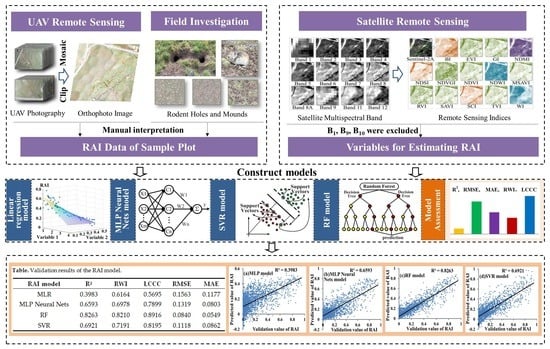
| RAI Model | R2 | RWI | LCCC | RMSE | MAE |
|---|---|---|---|---|---|
| MLR | 0.3983 | 0.6164 | 0.5695 | 0.1563 | 0.1177 |
| MLP Neural Nets | 0.6593 | 0.6978 | 0.7899 | 0.1319 | 0.0803 |
| RF | 0.8263 | 0.8210 | 0.8916 | 0.0840 | 0.0549 |
| SVR | 0.6921 | 0.7191 | 0.8195 | 0.1118 | 0.0862 |
Disclaimer/Publisher’s Note: The statements, opinions and data contained in all publications are solely those of the individual author(s) and contributor(s) and not of MDPI and/or the editor(s). MDPI and/or the editor(s) disclaim responsibility for any injury to people or property resulting from any ideas, methods, instructions or products referred to in the content. |
© 2023 by the authors. Licensee MDPI, Basel, Switzerland. This article is an open access article distributed under the terms and conditions of the Creative Commons Attribution (CC BY) license (https://creativecommons.org/licenses/by/4.0/).
Share and Cite
Dong, G.; Xian, W.; Shao, H.; Shao, Q.; Qi, J. Performance of Multiple Models for Estimating Rodent Activity Intensity in Alpine Grassland Using Remote Sensing. Remote Sens. 2023, 15, 1404. https://doi.org/10.3390/rs15051404
Dong G, Xian W, Shao H, Shao Q, Qi J. Performance of Multiple Models for Estimating Rodent Activity Intensity in Alpine Grassland Using Remote Sensing. Remote Sensing. 2023; 15(5):1404. https://doi.org/10.3390/rs15051404
Chicago/Turabian StyleDong, Guang, Wei Xian, Huaiyong Shao, Qiufang Shao, and Jiaguo Qi. 2023. "Performance of Multiple Models for Estimating Rodent Activity Intensity in Alpine Grassland Using Remote Sensing" Remote Sensing 15, no. 5: 1404. https://doi.org/10.3390/rs15051404