Next Article in Journal
ResiDualGAN: Resize-Residual DualGAN for Cross-Domain Remote Sensing Images Semantic Segmentation
Previous Article in Journal
A Bibliometric and Visualized Analysis of Remote Sensing Methods for Glacier Mass Balance Research
 
 
Correction published on 4 January 2024, see Remote Sens. 2024, 16(1), 206.
Article

Spatial Diffusion Waves of Human Activities: Evidence from Harmonized Nighttime Light Data during 1992–2018 in 234 Cities of China

1
Department of Land Resource Management, School of Public Administration, China University of Geosciences, Wuhan 430074, China
2
Key Labs of Law Evaluation of Ministry of Land and Resources of China, 388 Lumo Road, Hongshan District, Wuhan 430074, China
3
Collaborative Innovation Center for Emissions Trading System Co-Constructed by the Province and Ministry, Hubei University of Economics, Wuhan 430205, China
4
School of Low Carbon Economics, Hubei University of Economics, Wuhan 430205, China
*
Author to whom correspondence should be addressed.
Remote Sens. 2023, 15(5), 1426; https://doi.org/10.3390/rs15051426
Submission received: 28 December 2022 / Revised: 17 February 2023 / Accepted: 26 February 2023 / Published: 3 March 2023 / Corrected: 4 January 2024

Abstract

:
This study investigates whether the intensity of human activities conducted by urban populations and carried by urban land follows a wave-shaped diffusion rule using a harmonized DMSP-like NTL dataset during 1992–2018 in 234 cities of China. The results show that variations in the intensity of human activities are diffused in a wave-shaped manner from the urban center to the periphery in cities of different sizes and structures. The results demonstrate that variations in the intensity of human activity also exhibit a wave-shaped diffusion pattern, which is best modeled by a Gaussian function with an average R2 of 0.79 and standard deviation of 0.36 across all fitted functions. The outward movement of these waves in monocentric cities with an urban population <8 million occurred at a pace of ~0.5–1.0 km per year, reaching an average distance of ~18 km from the urban centers. While the pace decreased to ~0.2–0.6 km per year in larger or polycentric cities, the average distance of the waves from the urban centers increased to ~22–25 km in these larger cities. In addition, a process-pattern link between the distance-decayed rule and the wave-shaped rule of human activity dynamics was established. Moreover, a spatiotemporal Gaussian function was further discussed to enable modelers to forecast future variations in the intensity of human activities. The disclosed wave-shape rule and model can benefit the simulation of urban dynamics if integrated with other simulation technologies, such as agent-based models and cellular automata.

1. Introduction

During the past decades, considerable attention has been directed toward explanation theories or simulation models regarding urban dynamics, including patterns and variations of urban population [1,2], composition and configuration of urban land [3], and dynamics in the intensity of human activities [2,4]. Numerous models have been proposed to relate the local density of urban population or urban land to a distance-driven variable [5] such as the distance to urban centers [6], existing developments [7], or seeds of new developments [8]. However, there has been comparatively little research focused on developing rules and models that can explain the spatial and temporal variations in the intensity of human activities, despite the importance of understanding these variations for sustainable urban planning and management in a rapidly urbanizing world.
The relentless expansion of urban development towards the fringes of American and European cities over the past few decades has attracted the attention of many urban geographers who are now studying the patterns and processes of urban dynamics in these western cities [9,10,11,12,13,14]. The variations in the density of urban population and urban land have been shown to provide critical information on the processes, mechanisms, driving forces, structures, and stages of urban development, and have been widely analyzed. For example, Schneider and Woodcock [10] identified the urban cores as a circular region with a density of urban land greater than 50%, and partitioned the remaining areas using concentric rings of 8 km width, based on urban land density analysis. The tidal wave phenomenon of urban population density reveals the gentrification or suburbanization of urban development in metropolitan areas [15], and the position of the wave in relation to urban centers, to some extent, indicates the stages of urban development [16].
The outward, wavelike shifting of the urban population from the urban centers to the periphery has been widely observed in many metropolitan areas [11,15,17,18,19,20] and was quantitatively analyzed to demonstrate urban development properties since it was first observed by Blumenfeld [15] in the Philadelphia metropolitan area. Later, Newling [16] revealed the wave-shaped phenomenon manifested in spatial variations of urban population density and compared several mathematical functions to simulate this wave-shaped diffusion process. Finally, Newling prioritized the quadratic exponential and linear gamma functions and further formulated a density-profile classification scheme to describe the different stages of urban development. Investigation of the movement of urban population in Phoenix’s urban fringe areas disclosed the spatiotemporal structures of urban fringes in metropolitan areas and also confirmed the wavelike diffusion process of urban population in these areas [11]. Moreover, Parr [21] examined the form of regional population density using three mathematical functions and, finally, concluded that only the lognormal function appears to be capable of reflecting the density crater phenomenon that occurs in city centers during urban development.
With readily available data on urban land use over the last decade [22,23], researchers have been able to analyze density variations of urban land to better understand the properties of urban development. Earlier studies on urban land density mainly described density-related variables of urban land in regions or rings of different distances from urban centers [24,25] or existing urban areas [17]. Jiao [6] discovered a universal and spatially explicit rule for the distance-decayed variation in urban land density and proposed an inverse S-shape function to mathematically describe the rule, the first profile systematically characterizing the spatial variations in urban land density. Later, researchers developed a geographic microprocess model from a process-oriented viewpoint to quantify the urban expansion pattern of 112 large cities around the world [26]. The model explained how the inverse S-shape decreasing rule of urban land density emerges from a sequence of urban expansion processes in the microscale. More recently, Yang et al. [27] revealed that the physical-spatial process of urban expansion presents a wave-shaped diffusion regularity in terms of the density of new urban land, and can be well simulated with a Gaussian-based model instead of the inverse power function used in the geographic microprocess model proposed by Jiao, Dong, Xu, Zhou, Liu, and Liu [26].
While there has been significant advancement in comprehending the spatiotemporal dynamics of urban population and urban land density, including the wave-shaped rule that governs their dynamics, there has been a general neglect of the variations in the intensity of human activities resulting from these dynamics. This could be attributed, in part, to the absence of accurate and precise data on the distribution, intensity, and variations of large-scale human activities in the past decades, until the emergence of satellite-based nighttime light (NTL) data [28,29], i.e., the Defense Meteorological Satellite Program Operational Linescan System (DMSP-OLS) stable NTL data and the Suomi National Polar-orbiting Partnership Visible Infrared Imaging Radiometer Suite (NPP-VIIRS) NTL data [30]. Studies have already verified that it is plausible to utilize NTL data to investigate the spatiotemporal patterns and alterations of human activities from global to local scales [31,32,33]. Strong correlations were discovered between the luminosity of NTL and the intensity of human activities in space and time, such as the growth of the economy [34], consumption of energy [35], levels of urbanization [36], movement of urban residents [36], and many other urban-related elements on the global, national, regional, and local levels. In particular, the synchronous or asynchronous development between urban land and urban-related human activities were investigated based on NTL data in many regions [2,37,38,39].
Evidence from NTL data has demonstrated the spatiotemporal coordination among the density of urban population, distribution of urban land, and intensity of human activities [38]; however, whether the intensity of human activities also exhibits the same wave-shaped diffusion pattern as the density of urban population and urban land over space and time remains unverified. Therefore, this study provides an empirical understanding of the space–time pattern of human activities across 234 cities in China from 1992–2018 using a harmonized NTL dataset in order to verify whether the wave-shaped diffusion phenomenon also holds true in terms of variations in intensity of human activities, and to develop a quantitative model to explain it. Further discussion of the potential application of the rule and model, in regard to urban development and urban planning, was held as well.
The remaining parts of the paper are organized as follows: Section 2.1 describes the collection and preprocessing of datasets; Section 2.2 details the relevant methods; Section 3 shows and simulates the empirically observed waves of human activities in the sample cities; Section 4 discusses the possible applications of the proposed model and the contributions of the study; and Section 5 presents the conclusions that were drawn.

2. Materials and Methods

2.1. Sample Cities

In Figure 1, we displayed the 234 prefecture-level cities in China that were chosen for our study. These cities had a total population of over two million in 2020. Due to their vast quantity and lack of notable population growth and urban development, we excluded smaller cities and counties with populations below two million. The selected cities have all experienced obvious urban expansion in recent decades. Furthermore, the level of human activity intensity fluctuates considerably across time and space in both rural and urban areas of the chosen cities. The total population and urbanization degree of these cities varies greatly. Additionally, the landscape and spatial structures of the urbanized areas in these selected cities differ greatly. Table S1 in Supplemental Materials characterizes these cities in detail.
Among these cities, 44 cities have an urbanization rate larger than 70%. The largest cities, such as Beijing and Shanghai, have a total population greater than 20 million. The urbanization degree in these post-urbanization cities has surged in the past decades. For example, the urbanization degree of Beijing increased from 73.5% in 1990 to 86.60% in 2019, and that of Shanghai increased from 67.4% to 91.16% during this period. Most of these supercities are provincial capitals, and mainly located in central, eastern, and coastal areas of China (see Figure S1 in Supplemental Materials). A majority of the selected cities (184) are in the middle stage of urbanization, possessing an urbanization degree between 30%–70%. Among these middle-urbanization cities, Chongqing has the most urban residents, nearly 20 million, with an urbanization degree of 66.78% in 2019; while the least urbanized cities have an urban population of only 0.82 million, with an urbanization degree approaching 36.48%. There are also 6 cities that are in the early stage of urbanization, with an urbanization degree below 30%. Among these early-urbanization cities, Huanggang is the largest one, with a total population of 6.33 million and an urban population of only 1.57 million in 2019; the smallest one holds an urban population of merely 0.81 million.
Most of the selected cities are monocentric. The urbanized areas in these monocentric cities usually expand through adjacent or suburban development, forming the urbanized areas in a circlelike pattern. Accordingly, the urban population in these cities often diffuses outward like a tidal wave. These cities are mainly located in the central and eastern plains of China. Most polycentric cities expand their urban areas outward from each center through extension and sprawl development. As a consequence, these cities possess several clusters of urban population, each diffused from the center to the periphery. These polycentric cities, in most cases, are located in the plain regions of central and eastern China, and often have natural barriers (such as mountains, lakes, or rivers) between each cluster. Additionally, some polycentric cities enlarge their urban areas through linear development, resulting in a ribbonlike shape of the urbanized area. The spatial pattern of urban expansion and population growth in these cities of ribbon-shaped growth is usually formed by an existing corridor (such as a highway or a mountain valley) or barrier (such as a coast line or a river). Most of these cities of ribbon-shaped growth are located in the mountainous and hilly areas of northwestern and southwestern China.

2.2. Data and Preprocessing

In this study, we used harmonized and integrated global DMSP-like NTL data across a long time span, from 1992 to 2018, to indicate the intensity of human activities. This harmonized global NTL dataset was generated following four major steps [40]. First, the monthly NPP-VIIRS radiance data were composited to obtain an annual VIIRS dataset from 2012 to 2018. The composition operations also excluded temporal lights, such as aurora, fires, and boats. Second, DMSP-OLS data in different years from different sensors were interannually calibrated to eliminate the temporal inconsistency in the original DMSP data [41], thus generating temporally consistent DMSP time series data for NTL from 1992 to 2013. Third, a sigmoid model was trained based on the composited annual VIIRS and the interannually calibrated DMSP data from 2013 to establish the transformation relationship between the VIIRS and the DMSP NTL data. Fourth, the trained sigmoid model was applied at the global scale to convert the annual VIIRS data to DMSP-like data. The conversion procedure includes a spatial aggregation operation to down-sample the VIIRS data to the same spatial resolution (i.e., 30 arc-seconds) as the DMSP data using the kernel density approach, and a region-differentiated projection operation to convert the radiance values from VIIRS to DMSP-like digital number (DN) values based on the sigmoid model. Finally, the temporally consistent DMSP data from 1992 to 2013 and the converted DMSP-like data from 2014 to 2018 were concatenated to create the harmonized global DMSP-like NTL data from 1992 to 2018. These harmonized NTL data have a spatial resolution of 30 arc-seconds (about 1 km near the equator) and record the DN values, ranging from 0 to 63, to indicate the intensity of city light at night. We resample these harmonized DMSP-like NTL data to a spatial resolution of 30 m for further usage.
In addition to the harmonized NTL data, we also utilized impervious surface (ISA) data and the extent of functional urban areas to locate urban centers within a city. The ISA is regarded as the area that sustains human activities in the urban and rural regions of a city. In this study, we selected a global-scale ISA dataset mapped in 30 m resolution by considering the consistency and inconsistency of several existing products of global ISA. For consistent grids, an automagical machine-learning driven method was applied to classify these grids based on training samples extracted from the consistent regions of existing products. For the inconsistent grids, manually interpreted samples were added to the classification model to enhance its accuracy. The final classification accuracy of this global ISA dataset is 0.935, measured using F1 score. Details on how the ISA dataset was mapped are provided by Huang et al. [42]. The extent of the functional urban areas of global cities were identified based on an ISA dataset (30 m resolution) mapped in 2018 [22] using a cellular-automata model and morphological operations of dilating and eroding [43]. Other data used in this study include urban planning maps obtained from the official websites of the Bureau of Natural Resources, and total and urbanized population statistics collected from statistical yearbooks of each city. Table 1 provides an overview of the datasets used in this study.

2.3. Methodologies

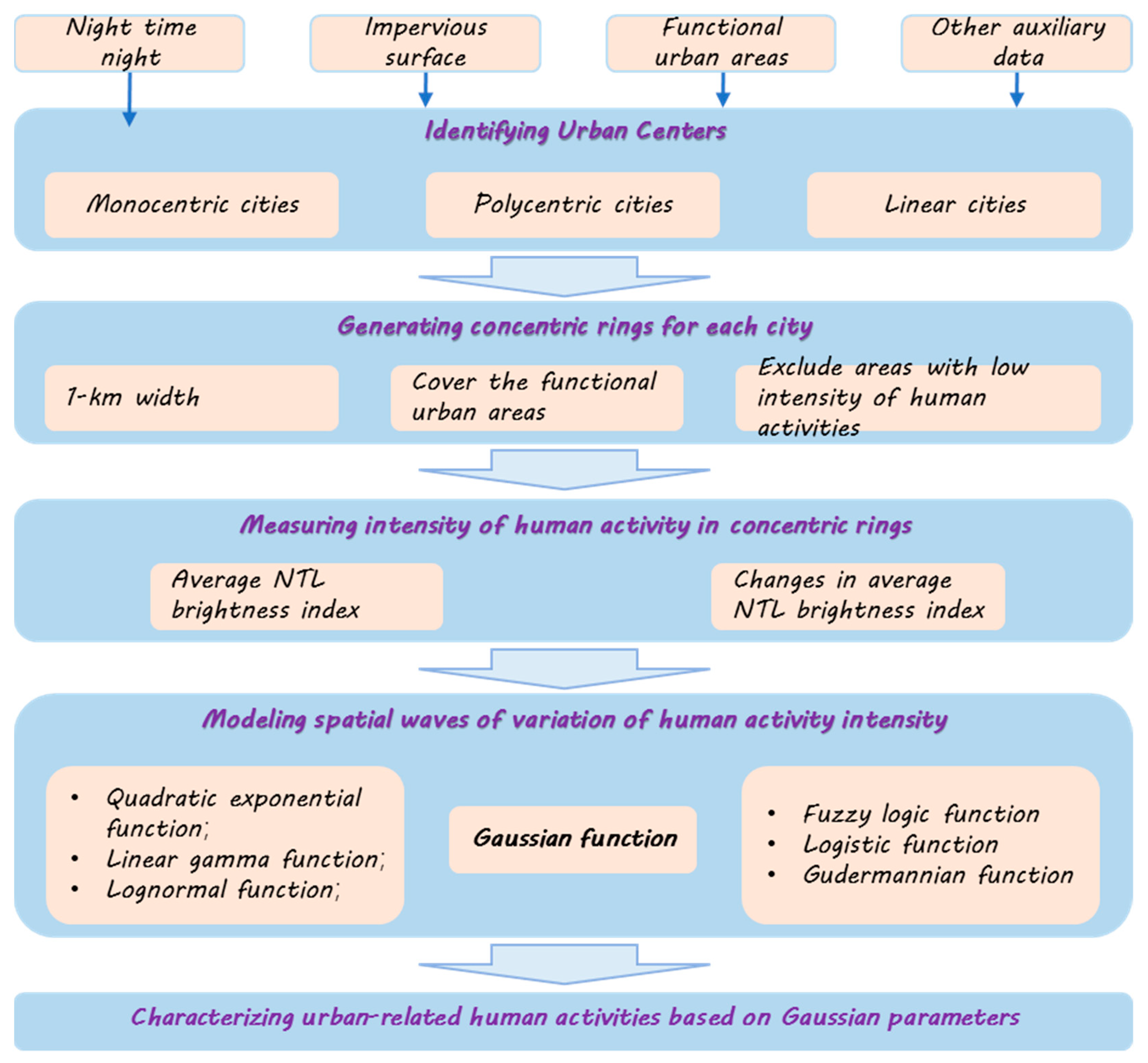
In this study, we employed various datasets, including nighttime satellite imagery, impervious surface data, and functional urban area data, to identify urban centers in different cities. From there, concentric rings were generated to analyze the gradient of human activity in each city. Then, the average brightness index calculated from nighttime light data was used to depict the intensity of human activity in each ring. Afterward, spatial waves in the variations of human activity intensity were visually presented and modeled using a Gaussian function, which was compared to six other bell-like functions for prioritization. Ultimately, the Gaussian function was prioritized to characterize urban-related human activity in the sample cities. Figure 2 provides an overview of the methodology used in this study.

2.3.1. Identifying Urban Centers for Each City

We located urban centers of each city typically based on the kernel density of ISA and NTL. First, we extracted the ISA and NTL data in 2018 using the administrative boundaries of each city. Afterward, the kernel density of ISA and NTL was calculated with bandwidth, automatically decided based on Silverman’s rule of thumb [44]. The foci points of these spatial kernels from the ISA and NTL dataset serve as the candidates for urban centers in a city. Then, we overlapped the extent of the functional urban areas of a city onto the kernel density maps to exclude small kernels distributed outside of the urbanized regions. The foci points that were located closest to the centers of large spatial continuums of ISA and NTL were retained for further identification. Third, we post-processed the retained foci points, based on expert knowledge and auxiliary data, to pick out the final urban centers. In most cities, a large spatial continuum of ISA and NTL is unique and should be easy to identify. Thus, there should be only one foci point identified based on ISA and NTL. Often, the two points extracted from ISA and NTL were close to each other. In this case, we arbitrarily retained one as the urban center. If there was more than one large spatial continuum from ISA and NTL in a city, we referred to its urban planning data to decide which large spatial continuum to retain for the selection of urban centers. In this process, expert knowledge and experience on the city’s urban development history played an important role. When the final spatial continuums were identified, we chose one focal point for each continuum, and adjacent foci points were combined. Finally, we located urban centers for all sample cities and produced a dataset for later use. Among the 234 cities, 135 had only one urban center, including Chengdu, Hefei, and Beijing. Among the 99 polycentric cities, 57 possessed 2 urban centers (including Tianjin and Weihai), 29 had 3 centers (including Wuhan and Guangzhou), and only 13 had 4 centers (including Nanjing and Hangzhou).

2.3.2. Generating Concentric Rings for Each City

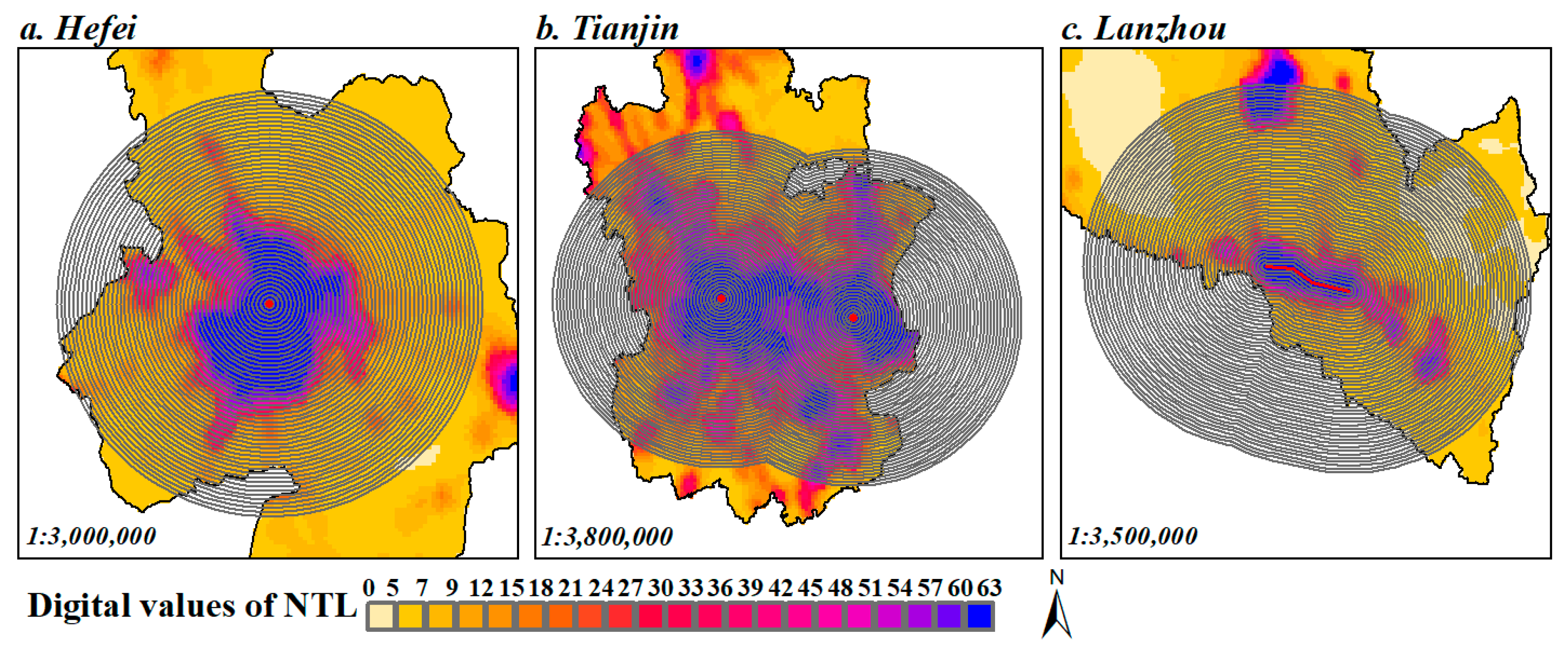
Using a set of concentric rings buffered outward from the urban centers (or axis) to the urban fringes, we applied a gradient-based approach to investigate the spatiotemporal diffusion processes of human activities. In all cities, the concentric rings had the same width, 1 km, as in many existing studies on spatiotemporal dynamics of urban land and urban population across the urban-to-rural gradients [45,46]. The farthest ring in a city should have an appropriate spatial extent to at least cover its functional urban areas, but exclude areas with a low intensity of human activities that are far from the urban centers [6]. The concentric rings in each city should share the same urban centers, as shown in Figure 3a,b. For those cities demonstrating ribbon-shaped growth, the concentric rings shared the same spatial axes, as shown in Figure 3c. The spatial axis of a linear city is the line connecting its multiple urban centers.

2.3.3. Measuring Intensity of Human Activity in Concentric Rings

We quantified the intensity of human activities in each concentric ring using the average NTL brightness index, which can be calculated as follows:
N T L B k = 1 N k × D N m a x × d n = D N m i n D N m a x d n × N d n , k
where N T L B k is the average NTL brightness in a ring k, N k is the total number of pixels that are not occupied by water in a ring k, D N m i n is the lower limit of DN value to extract different levels of human activities, D N m a x is the maximum DN value (which is 63 in this study), d n is a DN value between D N m i n and D N m a x , and N d n , k is the number of lit pixels with DN value being d n within ring k. The average NTL brightness index N T L B k is closely related with the intensity of human activities within ring k [28]. Apparently, N T L B k is related to the number of lit pixels in ring k and the DN values within these pixels. If all non-water pixels in a ring have a maximum DN value (i.e., 63) then N T L B k should be 1, indicating very high intensity of human activities. This is often the situation around the urban centers. N T L B k should be 0 if no lit pixels exist in a ring. This should happen if we applied a threshold ( D N m i n ) to exclude low-intensity human activities that occurred in rural areas.
The variations of human activity intensity within a ring k during a time interval Δ t (i.e., between two years t 1 and t 2 , Δ t = t 2 t 1 ) can be indicated by changes in N T L B k during this time interval, which can be calculated as follows:
N T L B k Δ t = N T L B k t 2 N T L B k t 1
where N T L B k Δ t is the changes of average NTL brightness during Δ t , indicating variations of human activity intensity within ring k. N T L B k t 2 and N T L B k t 1 are the average NTL brightness within ring k in year t 2 and t 1 , respectively.

2.3.4. A Gaussian Function for Simulating Spatial Variations of Human Activity Intensity

We defined the following Gaussian function to quantitatively model the spatiotemporal variations in intensity of human activities within a time interval Δ t :
I ( k , d i s t k , Δ t ) = a Δ t × e ( d i s t k b Δ t ) 2 c Δ t 2 + d Δ t
where I ( k , d i s t k , Δ t ) depicts the variations in intensity of human activities observed during time interval Δ t within concentric ring k. Variable d i s t k represents the Euclidean distance from ring k to the nearest urban center (or urban axis). Parameter a Δ t , b Δ t , and c Δ t are the amplitude, mean, and standard deviation of the Gaussian function. d Δ t is a constant variable.
When representing variations of human activity intensity using this Gaussian model, a Δ t indicates the largest variations of human activity intensity during Δ t among all concentric rings, b Δ t locates the hot zone (consisting of a set of concentric rings) where human activities are mostly intensified during Δ t , and c Δ t indicates the extent of the hot zone. Many previous studies have suggested that the urban–rural transition zones are oftentimes hot zones of urban expansion and, thus, are places where apparent dynamics in human activity intensity were observed. Therefore, parameter b Δ t and c Δ t sometimes provide clues to delineate the urban–rural transition zones of city. Moreover, parameter b Δ t helps identify the general spatial extent of the functional urban areas of a rapidly growing city. We introduced a constant parameter d Δ t into the classic Gaussian function to represent the dynamics of background human activity intensity in rural areas. This parameter, to some extent, disentangles changes of human activity intensity in urban areas from that in rural areas. Furthermore, temporal variations of parameters b Δ t and c Δ t over multiple time intervals within a long period informs the spatiotemporal dynamics in the intensity of human activities, which helps infer the stage and characteristic of urban development in a city. For instance, a rapid increase in parameter b Δ t during a period may indicate rapid urban expansion, and a decreasing trend in parameter b Δ t may indicate redevelopment in areas that have been urbanized. Note that decrease in parameter b Δ t only suggests an inward move of human activities, not the decrease of the physical extent of functional urban areas in a city, since we focus on the changes in intensity of human activity instead of its absolute intensity. Changes in parameter c Δ t can reveal dynamics in concentration degree of variations in human activity. For example, a possible explanation of an increasing trend in parameter c Δ t is that the city may have entered a stage when development of new urban areas and redevelopment of urbanized areas coexists.
In addition to the above-mentioned Gaussian function, we also used another 6 bell-shaped functions to fit the wavelike variations of human activity intensity and compared their performance (R2) with the proposed Gaussian function. The quadratic exponential, linear gamma, and lognormal function were applied in previous studies to model the spatial variation in density of urban population [5,16,19,21] and, thus, were adopted in this study. We also involved another 3 bell-shaped functions in the comparison; these are derivatives of fuzzy logic, logistic, and Gudermannian functions. The formulas of these functions are detailed in Table 2. We use non-linear least squares algorithms to optimize function parameters when fitting these functions to the empirical waves of human activity intensity observed during 1992 and 2018, with the lower limit of DN values varying from 1 to 50, with an increase of 10, and the time interval varying from 1 year to 9 years, with an increase of 2 years. The independent variable is the Euclidean distance of the ring to urban centers and the dependent variable is the variations of human activity intensity (i.e., N T L B k Δ t ) within a ring k during the time interval Δ t . The maximum number of tries to determine optimal function parameters is 10,000, without guesses on the initial values and limitations on ranges of parameters.

3. Results

3.1. Space–Time Pattern of Observed Intensity of Human Activities

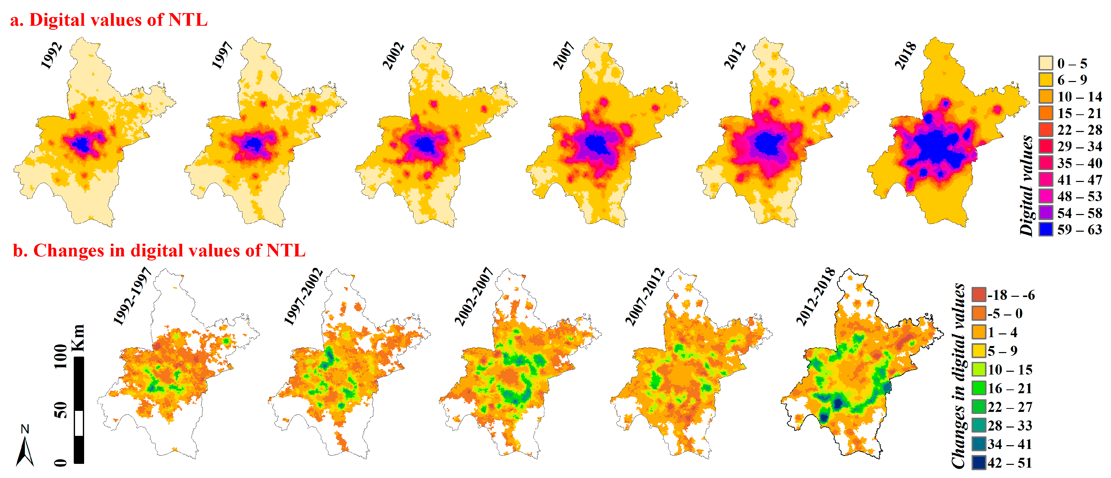
In the sample cities, there is a noticeable “center-periphery” pattern in the NTL data that corresponds with the consistent urban expansion processes from 1992 to 2018, particularly in metropolitan cities, as shown in a representative city, Wuhan (see Figure 4; other typical cities are referred to in Figures S2–S9 in Supplemental Materials). It can be seen that the high luminance areas are concentrated around the urban centers of a city and gradually expand outward over time (Figure 4a), which indicates the continuous diffusion of human activities from the urban cores to the fringe areas. Regarding changes in NTL over a duration, new lights in the sample cities were frequently lit up in the suburban regions of a city, leading to a pattern resembling a volcanic crater around the urban centers, as demonstrated by Figure 4b. This indicates that the rural–urban transition areas are oftentimes hotspots where human activities are mostly intensified. When examining changes in NTL across multiple time frames, new lights usually exhibit a gradual wave-shaped outward movement, similar to the spatial expansion of a “volcanic crater”. This wavelike process occurred during a long time span (such as 27 years in this study), suggesting a spatial diffusion phenomenon behind the dynamics of human activities.
The analysis based on concentric-ring gradient indicates that human activity intensity (i.e., N T L B k ) in the sample cities typically exhibits a distance-decay pattern within concentric rings, independent of the level of human activity (controlled by the lower limit of DN value). Nevertheless, the attenuation trajectory and rate of human activity intensity differ among cities and time periods. Figure 5 shows an example of the spatiotemporal pattern of human activity intensity within the concentric rings of a representative city, Wuhan (see more representative cities in Figures S10–S17 of the Supplemental Materials), when the lower limit of DN value is set to 1 or 30 (i.e., D N m i n = 1   o r   30 ). The N T L B k index indicates the total intensity of all-level human activities when D N m i n = 1 , and N T L B k indicates the total intensity of urban-related human activities when D N m i n = 30 . This threshold (DN = 30) is widely adopted in existing studies to extract human activities in urban areas [47] based on DMSP-like NTL data. What can be generally seen in Figure 5a,b is a decreasing trend in the total intensity of human activity from the urban centers to the outside areas in each year, regardless of the lower limit of DN value. If we focus on variations in the intensity of human activities (i.e., N T L B k Δ t ) within multiple time durations (e.g., a 5-year interval, Δ t = 5 ), concentric rings with larger variations (increasing) in intensity of human activity generally spread outward as waves spread ahead on open water, just like a ripple from a rock (or a stick, in cities with ribbon-shaped growth) thrown into a lake, as shown in Figure 5c,d. This pattern is often referred to as the “urban ripple effect.” The concentric rings of increasing intensity of human activity can be thought of as the “wave front” spreading outwards, with the central urban core representing the source of the “ripple”.
To further illustrate the observed spatiotemporal waves in variations of human activity intensity, we adopted a rolling strategy to calculate the average NTL brightness index ( N T L B k ) in concentric rings of each city. The rolling strategy of time uses overlapped time spans (such as 1992–1997, 1993–1998, and 1994–1999) to replace sequential time spans (such as 1992–1997, 1997–2002, and 2002–2007) to augment the dataset, thus demonstrating more details of continual changes in intensity of human activity. We also changed the length of time interval ( Δ t ) during each time span when calculating the variations of human activity intensity ( N T L B k Δ t ) to verify whether changes in temporal resolution would impact the wave-shaped patterns. In addition, we varied the D N m i n parameter to further investigate how dynamics in different levels of human activities change over space and time.
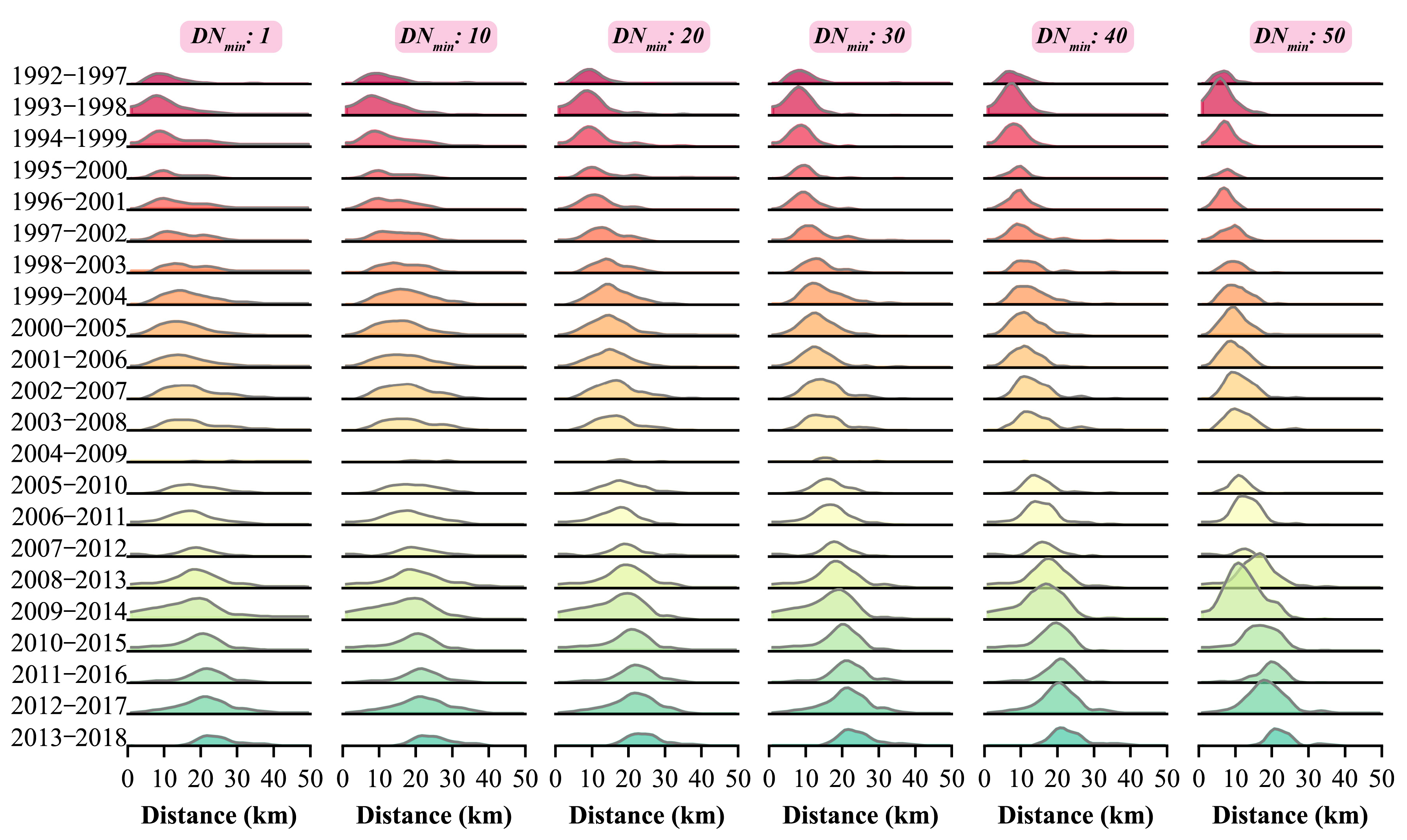
The results show that if we fixed the time interval, the spatial variation of human activity intensity during each interval clearly resembles a bell-shaped curve across rings, irrespective of the levels of human activities. However, the height, center, and width of these curves differ from one another. In general, at each level of human activity, the curve gradually expands outward, in waves, over time. However, the waves for low-intensity human activity seem to spread ahead slightly faster than waves of high-intensity human activities. In addition, the heights of the intensity curves tend to enlarge as we increase the lower limit of DN values to focus on higher levels of human activities, which, at the same time, narrows the curves of high-intensity human activities as well. This pattern is shown in Figure 6, which demonstrates the empirically observed wave of spatiotemporal variations in different levels of human activities in Wuhan from 1992 to 2018 when the D N m i n parameter varies from 1 to 50 and the time interval to calculate N T L B k Δ t is fixed at 5 years. Figures S18–S25 of Supplemental Materials illustrates the empirical waves of different levels of human activities in other typical cities. Notably, human activities in rural areas are generally stable. Therefore, the spatiotemporal variation in NTL of rural areas is small (close to 0). Additionally, the near-zero values in variations of human activity intensity within the urban cores may be caused by the saturation effect in the DMSP-like NTL data. However, this does not weaken the curve in reflecting the decreasing tendency in spatial variations of human activity intensity from the hot zones of new human activities (usually the urban–rural transition zones) to the urban cores.
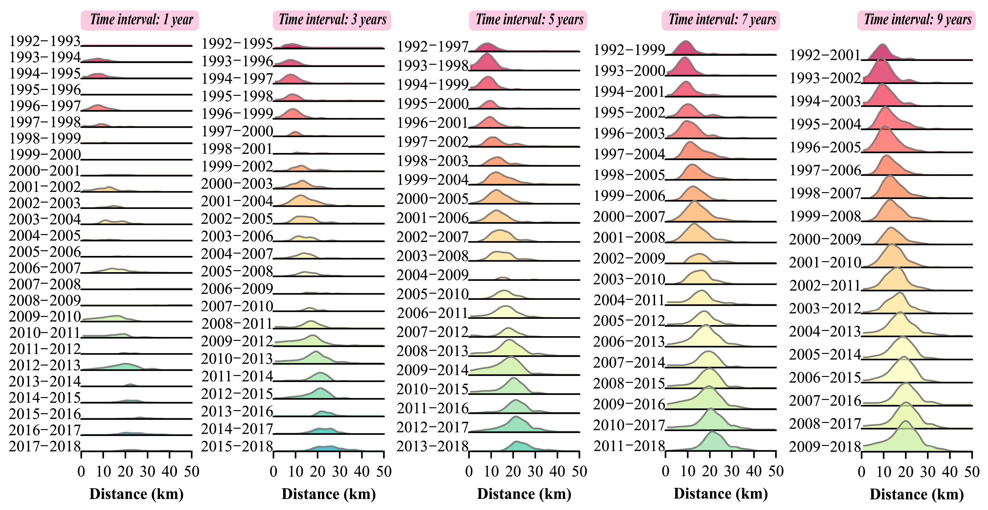
If we focus on a certain level of human activities (i.e., fix the lower limit of DN value), the wave-shaped diffusion pattern becomes more obvious when the time interval increases. On the contrary, a time interval that is too brief (e.g., 1 year) may overshadow the variations in NTL, and a 5-year lag seems to be a proper interval to investigate the spatiotemporal waves of human activity dynamics. Figure 7 shows how the length of time interval used to calculate N T L B k Δ t impacts the wave-shaped spatiotemporal pattern in variations of human activity intensity in Wuhan from 1992 to 2018 (see more representative cities in Figures S26–S32 of Supplement Materials) when the lower limit of DN values is fixed to 30, which is an acknowledged threshold to extract urban-related human activities based on DMSP-like NTL data.

3.2. Model Performance for Simulating Variations of Human Activity Intensity

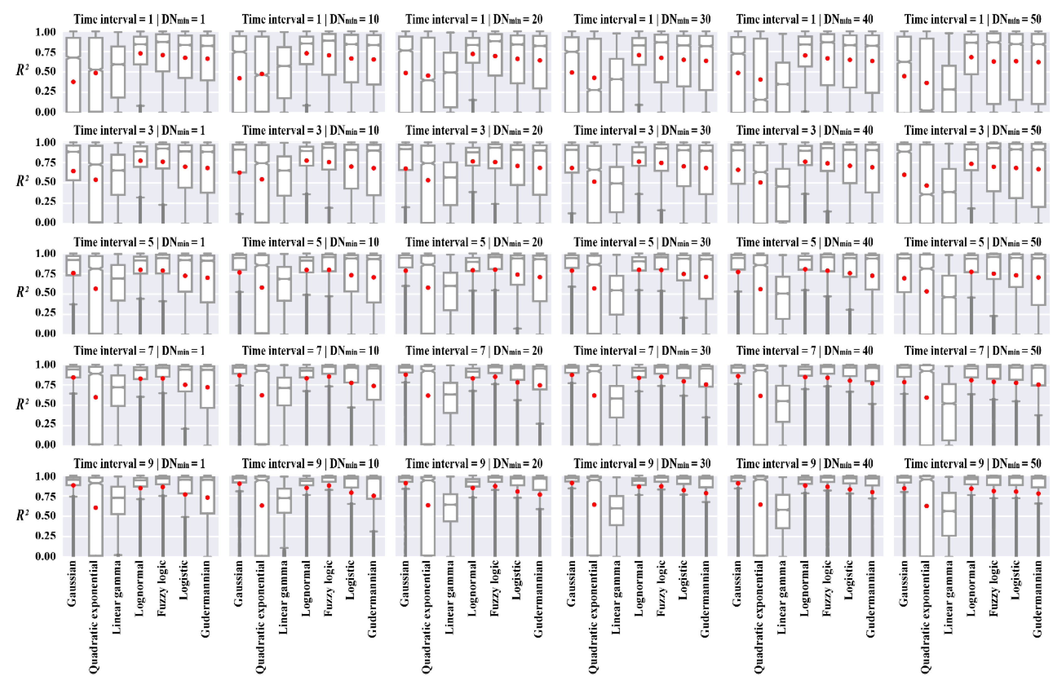
Figure 8 shows the boxplots for goodness of fit (R2) of the Gaussian function, as well as six additional bell-shaped functions, in modelling variations of human activity intensity. The results reveal that whatever function is used, there is an apparent increase in model performance (R2) when increasing time interval. When the time interval is fixed, R2 values for different functions change only slightly when fitting intensity variations in different levels of human activities. In particular, when the time interval is larger than 5 years, all functions fit the empirical waves well, with an average R2 approach of 0.75, except the quadratic exponential and linear gamma functions.
When we focus on urban-related human activities (i.e., D N m i n = 30 ) and fix the time interval to 5 years, the Gaussian, lognormal and fuzzy logic function have average R2 values of 0.79, 0.80, and 0.80, respectively, which are slightly higher than those of the logistic (0.74) and the Gudermannian (0.71) function, and much higher than that of the quadratic exponential (0.57) and linear gamma (fails to fit in most cases) functions. Although the fuzzy logic function has slightly higher average R2 than that of the Gaussian function, it more often failed to fit the waves (174 times out of 5148 times), while the Gaussian function fit all waves. The results found that the Gaussian function is generally a better way to model wave-shaped variations in human activity intensity, but other functions can be used depending on the situations. If the goal is to maximize the goodness of fit, a city-specific function should be chosen. However, if the focus is on characterizing human activity dynamics based on the fitted parameters, the Gaussian function is preferred, even though the lognormal function performs slightly better. This is because the Gaussian function has a more elegant form and spatially explicit geographical meaning in model parameters, unlike the lognormal function, which involves a logarithm operation that is difficult to explain intuitively.
Figure 9 details the R2 values of the Gaussian model when simulating variations in the intensity of urban-related human activities with the lower limit of DN values set to 30 ( D N m i n = 30 ) and the time interval set to 5 years ( Δ t = 5 ). The average R2 is 0.79, with standard deviation of 0.36, for all the fitted Gaussian models (#5148) for urban-related human activity. Nearly 76.76% of these fitted models have R2 values higher than 0.8, 81.64% have R2 values higher than 0.7, and only 13.81% have R2 values lower than 0.5. Nearly half of the sample cities have an average R2 higher than 0.8, and only 5 cities have an average R2 lower than 0.5. The maximum and minimum mean R2 is 0.98 (city of Laibin) and 0.22 (city of Jincheng), respectively, among the sample cities. For the 22 time periods (using the rolling strategy), more than half show average R2 larger than 0.8, with a maximum of 0.94, and only 1 time period (2013–2018) shows an average R2 lower than 0.5. The average R2 values tended to decline slightly as time passed, but the city size (indicated by urban population) seems to impose only moderate impact on model performance.
Although the Gaussian function generally performs well on average, its performance can vary considerably for individual cities and time periods. The varying model performance was not surprising, given that human activity variations that occur over short intervals are nonstationary across space and time, and can be influenced by a range of city-specific factors, including geographical conditions, transportation infrastructure, access to resources, natural barriers, and government policies, among other things. In general, monocentric cities undergoing rapid urbanization are more amenable to exhibiting a wave-shaped diffusion pattern in the variations of human activity intensity, making them more suitable to be simulated by the Gaussian function. However, small cities experiencing slow urban growth and supercities undergoing large urban renewal developments, in certain periods, may deviate from the wave-shaped diffusion pattern and may, therefore, show poor model performance. Additionally, polycentric and linear cities, where urban expansion is blocked by physical barriers such as the ocean and mountain ranges, generally demonstrate inferior performance compared to monocentric cities. Nonetheless, the results obtained from analyzing the sample cities during the period from 1992 to 2018 provide evidence supporting the Gaussian model’s ability to quantitatively model the wave-shaped processes of spatiotemporal variations in human activity intensity.

3.3. Characterizing Urban-Related Human Activities Based on Gaussian Parameters

Figure 10 depicts the average variations in Gaussian parameters b and c for cities with different sizes and spatial structures. Generally, larger cities exhibit higher values in parameter b (see subplots 1 and 2 in Figure 10), but the trend is less pronounced in parameter c. Although there are fluctuations, monocentric cities with an urban population of less than eight million exhibit a relatively stable trend with a slight increase in the mean values of parameter b. The outward movement of waves in these cities occurred at a pace of approximately 0.5–1.0 km per year, reaching an average distance of around 18 km from the urban centers (refer to subplot 1 in Figure 10). Conversely, parameter b in monocentric cities with an urban population exceeding eight million generally displays more fluctuations over time. In particular, parameter b of monocentric cities with an urban population exceeding 10 million has been experiencing a fluctuant downward trend on average since 1998. This downward trend also manifests in cities with an urban population between 8 and 10 million, after a relatively stable trend of rapid increase (compared to other monocentric cities) before 2008. During this period, the waves of these cities moved outward at a pace of almost 0.3–0.6 km per year, reaching an average distance of approximately 25 km from the centers. In contrast, polycentric cities with two urban centers of various sizes generally exhibit fewer fluctuations in parameter b over time, except for a sudden decrease in cities with an urban population between six and eight million. The waves of these polycentric cities typically move outward at a pace of approximately 0.2–0.5 km per year, reaching an average distance of about 14 km from the centers. Notably, Figure 10—2 highlights the more stable trend and fewer variations in parameter b for polycentric cities with an urban population exceeding 10 million, compared to polycentric cities of the same size. During this period, the waves of these polycentric cities moved outward at a pace of almost 0.4–0.6 km per year, reaching an average distance of approximately 22 km from the centers.
The analysis of parameter b suggests that small and mid-size Chinese cities (with an urban population of less than 8 million) are experiencing rapid urban expansion, while large cities with an urban population between 8 and 10 million are in a phase where urban expansion and redevelopment coexist (supported by the increasing trend in parameter c). On the other hand, supercities with an urban population exceeding 10 million are entering a renewal stage, evidenced by the declining trend in parameter b and the increasing trend in parameter c. The difference in parameter b between monocentric and polycentric supercities (with two urban centers) with an urban population exceeding 10 million could be due to monocentric cities’ tendency to enhance the population-carrying capacity of previously urbanized areas, while polycentric cities can relieve population pressure by utilizing another urban center. Thus, the extent of functional urban areas in each urban center is relatively small, allowing for further expansion of functional urban areas in monocentric cities, as evidenced by the increasing trend in parameter b (refer to subplot 2 in Figure 10).
Parameter c, in most time intervals, seems to show relatively little difference among cities with urban population < 10 million, irrespective of the number of urban centers (see subplots 3 and 4 in Figure 10). Monocentric supercities with an urban population >10 million tend to have slightly larger c values on the average, as well as larger variations among these supercities. The results suggest that although larger cities have a larger extent for functional urban areas, the extent for hot zones where human activities are mostly intensified does not differ significantly among cities with different sizes. Moreover, a sudden decrease is observed in parameter c of monocentric cities with an urban population between 8 and 10 million and of polycentric cities with an urban population between 6 and 8 million around the phase of 2010–2015, which is also the phase that the new-type urbanization strategy in China was released, in which urban expansion in large cities was limited and urban renewal was encouraged [48]. These changes, to some extent, suggest that urban development in these large cities is torn between the expansion-dominated and renewal-dominated strategy, which in most cases results in coexistence.
In addition, an overview of Figure 10 demonstrates that volatilities with different degrees occasionally appear in these parameters during different time intervals, especially in large cities. The results, in general, suggest that there exists nonstationarities over space and time in variations of human activity intensity observed in a short period (such as 5 years), particularly in larger cities with an urban population >6 million. In particular, the fluctuations seem to be enlarged in the past 10 years in large cities. This can be partially attributed to the release and execution of the new-type urbanization strategy. This strategy may cause urban planners and governors to wish to pursue both urban expansion and urban renewal in large and yet rapid-growing cities that still desire to and are capable to expand its functional urban areas [49,50]. If a city is still in a stage of urban expansion, such as monocentric cities with an urban population between six and eight million, but the local government chooses to follow the strategy, then urban expansion and renewal may coexist in these cities, which may lead to periodic decreases in parameter b and sudden increases in parameter c, as shown in subplot 2 and 4 in Figure 10. This situation can happen in polycentric large cities, since these cities have a stronger desire and larger capability to expand their functional urban areas. If the desire and impulsion of urban expansion finally overwhelm the political factors, then the city will continue to expand. Otherwise, it may gradually enter a renewal-dominated stage of urban development.

4. Discussion

4.1. Process-Pattern Linkage of Human Activities

The variations in the intensity of human activities within a time interval manifest a wave-shaped diffusion process. The spatiotemporal overlap and accumulation of sequential diffusion processes from an initial time point over space and time in a historical period will generate a distance-decay pattern in the total intensity of human activities at a final time point of interest, as evidenced by empirical observations from the sample cities. This relationship hints that we can link the wavelike diffusion processes to the spatial pattern of human activity in a specific time point based on the fitted models. Assuming that the intensity of human activity within a ring k at an initial time point t 0 is pre-known as N T L B k t 0 , then the intensity of human activity at the subsequent time point t 1 can be deduced to be N T L B k t 1 = N T L B k t 0 + ( 1 N T L B k t 0 ) N T L B k Δ t 1 , t 2 , i.e., 1 N T L B k t 1 = ( 1 N T L B k t 0 ) ( 1 N T L B k Δ t 0 , t 1 ) , where Δ t 0 , t 1 = t 1 t 0 and N T L B k Δ t 0 , t 1 is the changes in intensity of human activity during time period Δ t 0 , t 1 , which can be regarded as the possibility that new human activities will happen within ring k during Δ t 0 , t 1 . Similarly, we can calculate the intensity of human activity at the next time point t 2 as 1 N T L B k t 2 = ( 1 N T L B k t 0 ) ( 1 N T L B k Δ t 0 , t 1 ) ( 1 N T L B k Δ t 1 , t 2 ) . Therefore, the intensity of human activity at the final time of interest (depicted as t T ) can be recurrently deduced in the same manner, as follows:
N T L B k t T = 1 ( 1 N T L B k t 0 ) 0 T ( 1 N T L B k Δ t j 1 , t j ) ,   0 < j T
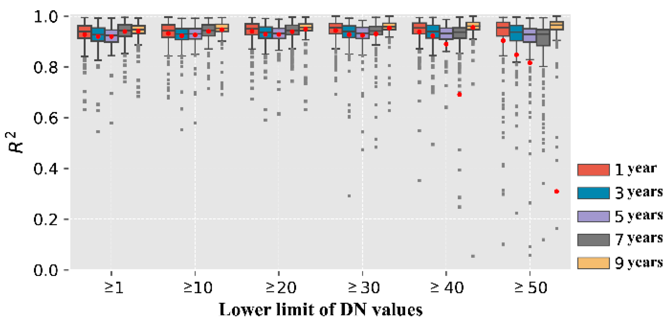
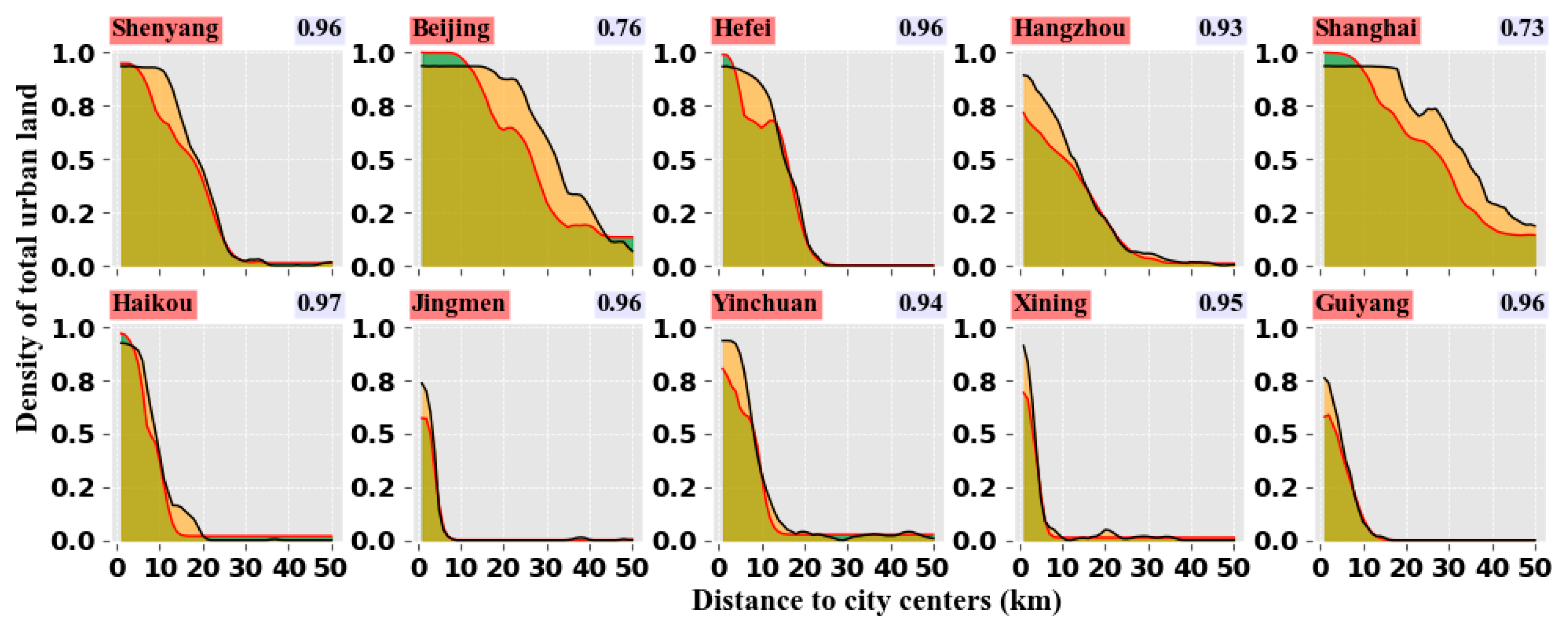
Figure 11 presents the degree of consistency (indicated using R2 values) between the observed and deduced patterns of total intensity of human activities of different levels based on the fitted Gaussian functions, with the time intervals ranging from 1 to 9 years. The initial and end time points during the deduction are 1992 and 2018, respectively. As can be seen in Figure 11, the deduced patterns of total human activity intensity, in most cases, match the observed patterns well. The average R2 reaches a high value of 0.93, with standard deviation of only 0.07. If we focus on urban-related human activities, the average R2 is 0.94 for different intervals of time, with standard deviation of 0.06. The deduced patterns for urban-related human activities in 10 typical cities of different sizes are shown in Figure 12. The results confirm that there exists a tight process-pattern linkage between the wave-shaped variations in intensity of human activity in the historical period and the distance-decayed patterns of total human activity intensity at a specific time point, which further support the feasibility of the Gaussian model in quantitatively representing the spatiotemporal processes of human activity variations.

4.2. A Prediction Model for Dynamics of Human Activity

Although the Gaussian function can fit and characterize the historical observations well, it is incapable of forecasting future variations in the intensity of human activity, given the temporal nonstationarities in Gaussian parameters, which weakens the applicability of the Gaussian model. In this regard, the Gaussian model should be related to the temporal dimension, in addition to its spatial dimension (i.e., distance to urban centers) to enable it to forecast future variations of human activity intensity. As for the four parameters of the Gaussian function, parameters b and c provide critical information on the dynamics of human activities. Additionally, results from the sampled cities suggest that parameter c shows less volatilities than parameter b, especially in rapidly growing cities. Therefore, for simplicity, we can keep the other three parameters as constant values and relate parameter b to time using a linear function, which will generate the following spatiotemporal Gaussian model:
I ( k , d i s t k , t ) = a × e ( d i s t k b t ) 2 c 2 + d
b t = b 0 + δ t   ( δ > 0 ) # ( 6 )
where t indicates continuous (instead of rolling) time intervals (i.e., t = 1 ,   2 ,   , n ) belonging to a long period of time: t 0 ~ t T . If the length of each time interval is Δ t , then t T t 0 Δ t = n . Parameter b t is the mean parameter of the Gaussian function for the tth time interval; b 0 is the b parameter at the initial time t 0 . Parameter δ is the changing rate of parameter b over time. Parameters a, c, and d remain consistent over all time intervals.
The spatiotemporal Gaussian model consists of a series of Gaussian functions with linearly increased b parameters and constant a, c, and d. These functions can be regarded as averaged surrogates of the spatiotemporal dynamics in the intensity of human activity. A critical question here is how to determine proper values for the parameters (i.e., a, c, d, b 0 , and δ ) of the spatiotemporal Gaussian model. This can be solved by calibrating the spatiotemporal Gaussian model based on the spatial pattern of the total intensity of human activities at the initial ( t 0 ) and end ( t T ) time point using an optimization algorithm and the process-pattern links described by Equation (4). The optimization problem can be formulated as follows:
m a x   F ( a ,   c ,   d ,   b 0   and   δ ) = c o n s i s t e n c y ( N T L B k t T ,   o b s e r v e d ,   N T L B k t T ,   d e d u c e d ) ,   k = 1 , 2 , , m
N T L B k t T ,   d e d u c e d = 1 ( 1 N T L B k t 0 ) 0 n ( 1 a × e ( d i s t k b 0 + δ t ) 2 c 2 + d ) , 0 < t n subject to :   0 < a < 1 ,   c > 0 , 0 < d < 1 ,   a n d   δ > 0
where c o n s i s t e n c y ( ) refers to the agreement degree between the observed ( N T L B k t T ,   o b s e r v e d ) and deduced ( N T L B k t T ,   d e d u c e d ) intensity of human activity within all rings at the end time point t T , which is indicated using R2. N T L B k t 0 is the observed intensity of human activity within ring k at the initial time point. The objective of the optimization problem is to maximize the agreement between the observed pattern of total human activity intensity and the pattern inferred using the spatiotemporal Gaussian model starting from an initial time point.

4.3. Wave-Shaped Phenomenon Manifested during Urbanization

Earlier research has demonstrated that urban population density exhibits a diffusion pattern resembling a wave over a long period of time, as per findings from previous studies [16,19,21]. This wave-shaped diffusion pattern was analyzed from a pattern-oriented standpoint by examining the distribution of urban inhabitants at specific moments. To a certain degree, our research indicates that the dispersion of fresh city inhabitants over a brief period could conform to a diffusion pattern shaped like a wave as well. This is because the fluctuations in human activity intensity are probably a consequence of these newcomers [11]. Additionally, earlier research indicates that urban land density declines from the urban core to the periphery at a specific point in time [6]. The physical expansion processes of new urban land that facilitates fresh human activities and shapes the distance-decay pattern of urban land density through intricate interaction and overlap over space and time follow a wave-shaped rule and can be represented using the Gaussian function as well [27]. Therefore, the “urban ripple effect” during urbanization can give rise to three wave-shaped phenomena: the distribution of new urban population, the allocation of new urban land, and variations in human activity intensity. Their inter-relationship can be understood as follows. First, as urban areas in a city expand outward, the early occupants on the newly developed urban land will light these places slightly in the beginning. Then, human activities will be largely intensified as more new residents move in, accompanied by more city infrastructure and public services over time. In this stage, these newly developed areas become hotspots for newcomers and fresh human activities, and the NTL will increase accordingly. Afterward, human activity in these places will gradually reach a saturation point as urban growth continues, and variation in the intensity of human activities will largely decrease. As cities continue to enlarge their urban areas, this process repeats in newly developed areas and diffuses outward from urban centers to the fringe areas.
An intriguing question that arises is whether the three types of waves exhibit similar patterns in space and time, with matching frequency and amplitude. One possible conjecture is that they are more likely to align, or exhibit fewer discrepancies, in cities experiencing rapid urban expansion and urbanization. In most situations, spatiotemporal discrepancies should exist among these waves in different places and periods, due to the influence of the natural barriers, land use regulations, location preference, or rapid suburbanization, among other factors [38]. While urban population growth often necessitates the expansion of urban land, the dynamics of these two processes differ. The expansion of urban land involves a physical-spatial transformation from nonurban to urban land, which is difficult to reverse. In contrast, the movement or diffusion of population to newly developed urban areas represents a “flow” that is fixed in space and time. In addition, urban population growth does not always cause the expansion of new urban land, as densification of urban population in the urban core can also occur. Likewise, although human activities in urban areas are conducted by urban residents and take place on urban land, intensification of human activities does not always coincide with an increase in urban population or expansion of urban land. This is especially true in highly urbanized cities, where the intensification of human activities can also result from ongoing improvements in living standards and investment in urban infrastructure and facilities. Examining the spatiotemporal discrepancies among these three wave patterns can uncover various urban issues, including the effectiveness of urban development, job–housing imbalances, and the occupation of agricultural land and open spaces. This information can help inform urban management and planning. For instance, if the wave of urban development in a city is expanding more rapidly than the waves of urban population or urban-related human activities, it may indicate disorderly urban development that requires regulation [2,37].

4.4. Major Contributions of This Study

This study’s primary contribution is revealing the wave-shaped diffusion phenomenon in the spatial variations of human activity intensity. The study also proposes a Gaussian model to quantitatively simulate and describe this phenomenon, offering novel perspectives and methods to analyze, explain, and model the spatiotemporal patterns of human activity and relevant factors, particularly in urban settings.
First, findings in this study complement existing theories on urban-related elements by adopting a “pattern-from-process” perspective to disentangle the spatiotemporal patterns of human activities into a series of underlying processes that occur within a short time interval. Previous studies have tended to adopt a “process-from-pattern” paradigm, which may obscure information hidden in the underlying processes. By proposing a quantitative model to directly characterize and simulate these processes, this study allows for a straightforward analysis of the mechanisms and biophysical and socioeconomic factors that impact human activity dynamics.
Second, the process-oriented Gaussian-based model for variations in human activity intensity can benefit modelers by offering new opportunities to simulate and predict the spatiotemporal patterns of human activity and related urban elements, such as population and land use. This is especially useful for cities undergoing rapid urbanization, as it enables urban planners to predict future hot zones of human activity and, thus, make informed decisions about urban infrastructure and facilities, protect valuable natural spaces, and prevent negative consequences. For example, the process-oriented diffusion rule provides new avenues to spatialize the total urban population of a city, based on the process-pattern links (discussed in Section 4.1), if the distribution of urban population at the initial time point is pre-known, which has long been a key challenge in the simulation community [51]. This process-oriented rule regarding human activities and urban population is particularly helpful in agent-based modeling of urban dynamics. Additionally, the spatiotemporal Gaussian model can guide the urban modelers to spatialize the urban demand of a time period into space (each ring) and time, which allows for subtle control of the macrolevel morphology of simulated urban landscapes from a process-oriented paradigm if integrated with a bottom-up simulation tool, such as the cellular automata model [52,53].

5. Conclusions

Based on nighttime light data spanning from 1992 to 2018 in 234 Chinese cities, this study has uncovered a diffusion pattern that resembles waves with regards to the variations in the intensity of human activity. The research indicates that hot zones with higher variability in the intensity of human activity typically shift outward from the urban core, similar to ripples in a lake caused by a thrown rock. The Gaussian function is more suitable for modeling this wave-shaped phenomenon, surpassing other bell-shaped functions, with an average R2 of 0.79 and a standard deviation of 0.36 across all the fitted Gaussian functions for urban-related human activities in the sample cities.
The outward movement of these waves of human activities in monocentric cities with an urban population < 8 million occurred at a pace of ~0.5–1.0 km per year, reaching an average distance of ~18 km from the urban centers. While the pace decreased to ~0.2–0.6 km per year in larger cities or polycentric cities, the average distance of the waves from the urban centers increased to ~22–25 km in these larger cities. The results also suggest that small and mid-size Chinese cities (urban population < 8 million) are experiencing rapid urban expansion, while large cities with an urban population between 8 and 10 million are in a phase where urban expansion and redevelopment coexist. Supercities with an urban population exceeding 10 million are entering a renewal stage. Urban planners can leverage the information about the size, shape, pace, and timing of these waves to arrange infrastructure and services.
The results of the model also suggest that while the intensity of human activities may fluctuate over time, it follows a wave-shaped hidden rule. Additionally, we demonstrated how the wave-shaped diffusion of human activities in historical periods can be linked to the distance-decayed spatial pattern of human activity in a specific time point using fitted Gaussian functions, which can aid in the spatialization of urban population and the simulation of urban expansion. A spatiotemporal Gaussian function was also proposed to enable us to forecast future changes in the intensity of human activities, significantly enhancing the model’s practicality in urban planning and simulation. Future research on this topic may involve exploring the degree to which the three types of waves (i.e., urban population, urban land, and human activities) correlate with each other and how their spatiotemporal discrepancies can inform us on urban management and planning.

Supplementary Materials

The following are available online at https://www.mdpi.com/2072-4292/15/5/1426/s1, Table S1: Detailed characteristics of the 234 sample cities, Figure S1: Landscape types and locations of the selected cities, Figures S2–S9: Spatiotemporal pattern of NTL in 8 representative cities, Figures S10–S17: Intensity of human activity within concentric rings of 8 representative cities when the lower limit of DN value to extract human activities is set to 1 and 30, and the interval of time is set to 5 years, i.e., Δ t = 5 , Figures S18–S25: Wave of spatiotemporal variations in different levels of human activities in 8 typical cities from 1992 to 2018 when and the time interval is fixed as 5 years and the D N m i n parameter vary from 1 to 50, Figures S26–S32: Wave of spatiotemporal variations in intensity of human activities in 8 typical cities from 1992 to 2018 when the when the D N m i n = 30 and the time interval varies from 1 to 9 years with increment of 2 years.

Author Contributions

J.Y.: Conceptualization, Methodology, Software, Writing—Original draft. M.Y.: Data collection, processing, analysis, visualization, and revision. D.Z. and S.Y.: Conceptualization, Methodology, Writing-Reviewing and Editing. Y.W.: Conceptualization, Writing—Original Draft. D.S.: Software, Visualization. Y.D.: Formal analysis, Writing—Reviewing and Editing. Y.G.: Formal analysis, processing, analysis. J.G.: Resources, Data curation, Funding acquisition, Supervision. All authors have read and agreed to the published version of the manuscript.

Funding

This study was supported by the National Natural Science Foundation of China (No. 42101275 and No. 42071254), and the Fundamental Research Funds for the Central Universities, China University of Geosciences (CUGL170408 and CUGGG-2020).

Data Availability Statement

We use open-access data in this study. Their availability is detailed in Table 1.

Acknowledgments

We thank the Center of big data and high-performance computing in Department of land resources management in China University of Geosciences (Wuhan), China for data collection and processing.

Conflicts of Interest

The authors declare no conflict of interest.

References

  1. Xu, G.; Jiao, L.; Yuan, M.; Dong, T.; Zhang, B.; Du, C. How does urban population density decline over time? An exponential model for Chinese cities with international comparisons. Landsc. Urban Plan. 2019, 183, 59–67. [Google Scholar] [CrossRef]
  2. Chen, Y.; Liu, X.; Li, X. Analyzing Parcel-Level Relationships between Urban Land Expansion and Activity Changes by Integrating Landsat and Nighttime Light Data. Remote Sens. 2017, 9, 164. [Google Scholar] [CrossRef]
  3. Aguilera, F.; Valenzuela, L.M.; Botequilha-Leitao, A. Landscape metrics in the analysis of urban land use patterns: A case study in a Spanish metropolitan area. Landsc. Urban Plan. 2011, 99, 226–238. [Google Scholar] [CrossRef]
  4. Zhang, X.D.; Wang, X.D.; Zhou, Z.X.; Li, M.W.; Jing, C.F. Spatial Quantitative Model of Human Activity Disturbance Intensity and Land Use Intensity Based on GF-6 Image, Empirical Study in Southwest Mountainous County, China. Remote Sens. 2022, 14, 4574. [Google Scholar] [CrossRef]
  5. Zielinski, K. Experimental analysis of eleven models of urban population density. Environ. Plan. A 1979, 11, 629–641. [Google Scholar] [CrossRef]
  6. Jiao, L. Urban land density function: A new method to characterize urban expansion. Landsc. Urban Plan. 2015, 139, 26–39. [Google Scholar] [CrossRef]
  7. Linard, C.; Tatem, A.J.; Gilbert, M. Modelling spatial patterns of urban growth in Africa. Appl. Geogr. 2013, 44, 23–32. [Google Scholar] [CrossRef]
  8. Meentemeyer, R.K.; Tang, W.; Dorning, M.A.; Vogler, J.B.; Cunniffe, N.J.; Shoemaker, D.A. FUTURES: Multilevel Simulations of Emerging Urban-Rural Landscape Structure Using a Stochastic Patch-Growing Algorithm. Ann. Assoc. Am. Geogr. 2013, 103, 785–807. [Google Scholar] [CrossRef]
  9. Thomas, I.; Frankhauser, P.; Biernacki, C. The morphology of built-up landscapes in Wallonia (Belgium): A classification using fractal indices. Landsc. Urban Plan. 2008, 84, 99–115. [Google Scholar] [CrossRef]
  10. Schneider, A.; Woodcock, C.E. Compact, Dispersed, Fragmented, Extensive? A Comparison of Urban Growth in Twenty-five Global Cities using Remotely Sensed Data, Pattern Metrics and Census Information. Urban Stud. 2008, 45, 659–692. [Google Scholar] [CrossRef]
  11. Gober, P.; Burns, E.K. The Size and Shape of Phoenix’s Urban Fringe. J. Plan. Educ. Res. 2002, 21, 379–390. [Google Scholar] [CrossRef]
  12. Dietzel, C.; Oguz, H.; Hemphill, J.J.; Clarke, K.C.; Gazulis, N. Diffusion and Coalescence of the Houston Metropolitan Area: Evidence Supporting a New Urban Theory. Environ. Plan. B Plan. Des. 2016, 32, 231–246. [Google Scholar] [CrossRef]
  13. Dietzel, C.; Herold, M.; Hemphill, J.J.; Clarke, K.C. Spatio-temporal dynamics in California’s central valley: Empirical links to urban theory. Int. J. Geogr. Inf. Sci. 2005, 19, 175–195. [Google Scholar] [CrossRef]
  14. Carlucci, M.; Ferrara, C.; Rontos, K.; Zambon, I.; Salvati, L. The long breadth of cities: Revisiting worldwide urbanization patterns, 1950–2030. Appl. Econ. 2020, 52, 4162–4174. [Google Scholar] [CrossRef]
  15. Blumenfeld, H. The Tidal Wave of Metropolitan Expansion. J. Am. Inst. Plan. 1954, 20, 3–14. [Google Scholar] [CrossRef]
  16. Newling, B.E. The spatial variation of urban population densities. Geogr. Rev. 1969, 59, 242–252. [Google Scholar] [CrossRef]
  17. Xu, C.; Liu, M.; Zhang, C.; An, S.; Yu, W.; Chen, J.M. The spatiotemporal dynamics of rapid urban growth in the Nanjing metropolitan region of China. Landsc. Ecol. 2007, 22, 925–937. [Google Scholar] [CrossRef]
  18. Morrill, R.L. Waves of Spatial Diffusion. J. Reg. Sci. 2010, 8, 1–18. [Google Scholar] [CrossRef]
  19. Koreclli, P. A wave-like model of metropolitan spatial growth. Pap. Reg. Sci. Assoc. 2010, 24, 127–140. [Google Scholar] [CrossRef]
  20. Hart, J.F. The Perimetropolitan Bow Wave. Geogr. Rev. 1991, 81, 35–51. [Google Scholar] [CrossRef]
  21. Parr, J.B. The form of the regional density function. Reg. Stud. 2007, 19, 535–546. [Google Scholar] [CrossRef]
  22. Gong, P.; Li, X.C.; Wang, J.; Bai, Y.Q.; Cheng, B.; Hu, T.Y.; Liu, X.P.; Xu, B.; Yang, J.; Zhang, W.; et al. Annual maps of global artificial impervious area (GAIA) between 1985 and 2018. Remote Sens. Environ. 2020, 236, 111510. [Google Scholar] [CrossRef]
  23. Gong, P.; Chen, B.; Li, X.; Liu, H.; Wang, J.; Bai, Y.; Chen, J.; Chen, X.; Fang, L.; Feng, S.; et al. Mapping essential urban land use categories in China (EULUC-China): Preliminary results for 2018. Sci. Bull. 2020, 65, 182–187. [Google Scholar] [CrossRef] [PubMed]
  24. Tsai, Y.-H. Quantifying Urban Form: Compactness versus ‘Sprawl’. Urban Stud. 2005, 42, 141–161. [Google Scholar] [CrossRef]
  25. Angel, S.; Parent, J.; Civco, D. Urban sprawl metrics: An analysis of global urban expansion using GIS. In Proceedings of the ASPRS 2007 Annual Conference, Tampa, FL, USA, 7–11 May 2007. [Google Scholar]
  26. Jiao, L.; Dong, T.; Xu, G.; Zhou, Z.; Liu, J.; Liu, Y. Geographic micro-process model: Understanding global urban expansion from a process-oriented view. Comput. Environ. Urban Syst. 2021, 87, 101603. [Google Scholar] [CrossRef]
  27. Yang, J.; Li, J.; Xu, F.; Li, S.; Zheng, M.; Gong, J. Urban development wave: Understanding physical spatial processes of urban expansion from density gradient of new urban land. Comput. Environ. Urban Syst. 2022, 97, 101867. [Google Scholar] [CrossRef]
  28. Gao, B.; Huang, Q.; He, C.; Ma, Q. Dynamics of Urbanization Levels in China from 1992 to 2012: Perspective from DMSP/OLS Nighttime Light Data. Remote Sens. 2015, 7, 1721–1735. [Google Scholar] [CrossRef]
  29. Zhang, X.S.; Xu, Z.J. Functional Coupling Degree and Human Activity Intensity of Production-Living-Ecological Space in Underdeveloped Regions in China: Case Study of Guizhou Province. Land 2021, 10, 56. [Google Scholar] [CrossRef]
  30. Zhao, M.; Zhou, Y.Y.; Li, X.C.; Cao, W.T.; He, C.Y.; Yu, B.L.; Li, X.; Elvidge, C.D.; Cheng, W.M.; Zhou, C.H. Applications of Satellite Remote Sensing of Nighttime Light Observations: Advances, Challenges, and Perspectives. Remote Sens. 2019, 11, 1971. [Google Scholar] [CrossRef]
  31. Ma, T. Multi-Level Relationships between Satellite-Derived Nighttime Lighting Signals and Social Media-Derived Human Population Dynamics. Remote Sens. 2018, 10, 1128. [Google Scholar] [CrossRef]
  32. Shi, K.F.; Huang, C.; Chen, Y.; Li, L.Y. Remotely sensed nighttime lights reveal increasing human activities in protected areas of China mainland. Remote Sens. Lett. 2018, 9, 468–477. [Google Scholar] [CrossRef]
  33. Lan, F.; Gong, X.Y.; Da, H.L.; Wen, H.Z. How do population inflow and social infrastructure affect urban vitality? Evidence from 35 large- and medium-sized cities in China. Cities 2020, 100, 102454. [Google Scholar] [CrossRef]
  34. Keola, S.; Andersson, M.; Hall, O. Monitoring Economic Development from Space: Using Nighttime Light and Land Cover Data to Measure Economic Growth. World Devel. 2015, 66, 322–334. [Google Scholar] [CrossRef]
  35. Zhu, Y.G.; Xu, D.Y.; Ali, S.H.; Ma, R.Y.; Cheng, J.H. Can Nighttime Light Data Be Used to Estimate Electric Power Consumption? New Evidence from Causal-Effect Inference. Energies 2019, 12, 3154. [Google Scholar] [CrossRef]
  36. Zhao, M.; Cheng, W.M.; Zhou, C.H.; Li, M.C.; Huang, K.; Wang, N. Assessing Spatiotemporal Characteristics of Urbanization Dynamics in Southeast Asia Using Time Series of DMSP/OLS Nighttime Light Data. Remote Sens. 2018, 10, 47. [Google Scholar] [CrossRef]
  37. Ma, T. An Estimate of the Pixel-Level Connection between Visible Infrared Imaging Radiometer Suite Day/Night Band (VIIRS DNB) Nighttime Lights and Land Features across China. Remote Sens. 2018, 10, 723. [Google Scholar] [CrossRef]
  38. Liu, Y.L.; Zhang, X.H.; Kong, X.S.; Wang, R.; Chen, L. Identifying the relationship between urban land expansion and human activities in the Yangtze River Economic Belt, China. Appl. Geogr. 2018, 94, 163–177. [Google Scholar] [CrossRef]
  39. He, X.; Li, Z.; Guo, H.; Tian, Z.; Wang, X. Analysing the consistency between built-up areas and human activities and the impacts on the urbanization process: A case study of Zhengzhou, China. Int. J. Remote Sens. 2019, 40, 6008–6035. [Google Scholar] [CrossRef]
  40. Li, X.; Zhou, Y.; Zhao, M.; Zhao, X. A harmonized global nighttime light dataset 1992–2018. Sci. Data 2020, 7, 168. [Google Scholar] [CrossRef]
  41. Li, X.C.; Zhou, Y.Y. A Stepwise Calibration of Global DMSP/OLS Stable Nighttime Light Data (1992–2013). Remote Sens. 2017, 9, 637. [Google Scholar] [CrossRef]
  42. Huang, X.; Song, Y.; Yang, J.; Wang, W.; Ren, H.; Dong, M.; Feng, Y.; Yin, H.; Li, J. Toward accurate mapping of 30-m time-series global impervious surface area (GISA). Int. J. Appl. Earth Obs. Geoinf. 2022, 109, 102787. [Google Scholar] [CrossRef]
  43. Li, X.; Gong, P.; Zhou, Y.; Wang, J.; Bai, Y.; Chen, B.; Hu, T.; Xiao, Y.; Xu, B.; Yang, J.; et al. Mapping global urban boundaries from the global artificial impervious area (GAIA) data. Environ. Res. Lett. 2020, 15, 094044. [Google Scholar] [CrossRef]
  44. Kemp, C.D.; Silverman, B.W. Density Estimation for Statistics and Data Analysis; Chapman and Hall: New York, NY, USA, 1987. [Google Scholar]
  45. Xu, G.; Jiao, L.; Liu, J.; Shi, Z.; Zeng, C.; Liu, Y. Understanding urban expansion combining macro patterns and micro dynamics in three Southeast Asian megacities. Sci. Total Environ. 2019, 660, 375–383. [Google Scholar] [CrossRef]
  46. Dong, T.; Jiao, L.; Xu, G.; Yang, L.; Liu, J. Towards sustainability? Analyzing changing urban form patterns in the United States, Europe, and China. Sci. Total Environ. 2019, 671, 632–643. [Google Scholar] [CrossRef]
  47. Zhao, M.; Xu, G.; de Jong, M.; Li, X.; Zhang, P. Examining the Density and Diversity of Human Activity in the Built Environment: The Case of the Pearl River Delta, China. Sustainability 2020, 12, 3700. [Google Scholar] [CrossRef]
  48. Chen, M.X.; Liu, W.D.; Lu, D.D.; Chen, H.; Ye, C. Progress of China’s new-type urbanization construction since 2014: A preliminary assessment. Cities 2018, 78, 180–193. [Google Scholar] [CrossRef]
  49. Long, H.L. Land consolidation: An indispensable way of spatial restructuring in rural China. J. Geogr. Sci. 2014, 24, 211–225. [Google Scholar] [CrossRef]
  50. Fang, C.L.; Wang, Z.B. Quantitative Diagnoses and Comprehensive Evaluations of the Rationality of Chinese Urban Development Patterns. Sustainability 2015, 7, 3859–3884. [Google Scholar] [CrossRef]
  51. Li, K.N.; Chen, Y.H.; Li, Y. The Random Forest-Based Method of Fine-Resolution Population Spatialization by Using the International Space Station Nighttime Photography and Social Sensing Data. Remote Sens. 2018, 10, 1650. [Google Scholar] [CrossRef]
  52. Yang, J.; Tang, W.; Gong, J.; Shi, R.; Zheng, M.; Dai, Y. Simulating urban expansion using cellular automata model with spatiotemporally explicit representation of urban demand. Landsc. Urban Plan. 2023, 231, 104640. [Google Scholar] [CrossRef]
  53. Wang, W.; Jiao, L.; Dong, T.; Xu, Z.; Xu, G. Simulating urban dynamics by coupling top-down and bottom-up strategies. Int. J. Geogr. Inf. Sci. 2019, 33, 2259–2283. [Google Scholar] [CrossRef]
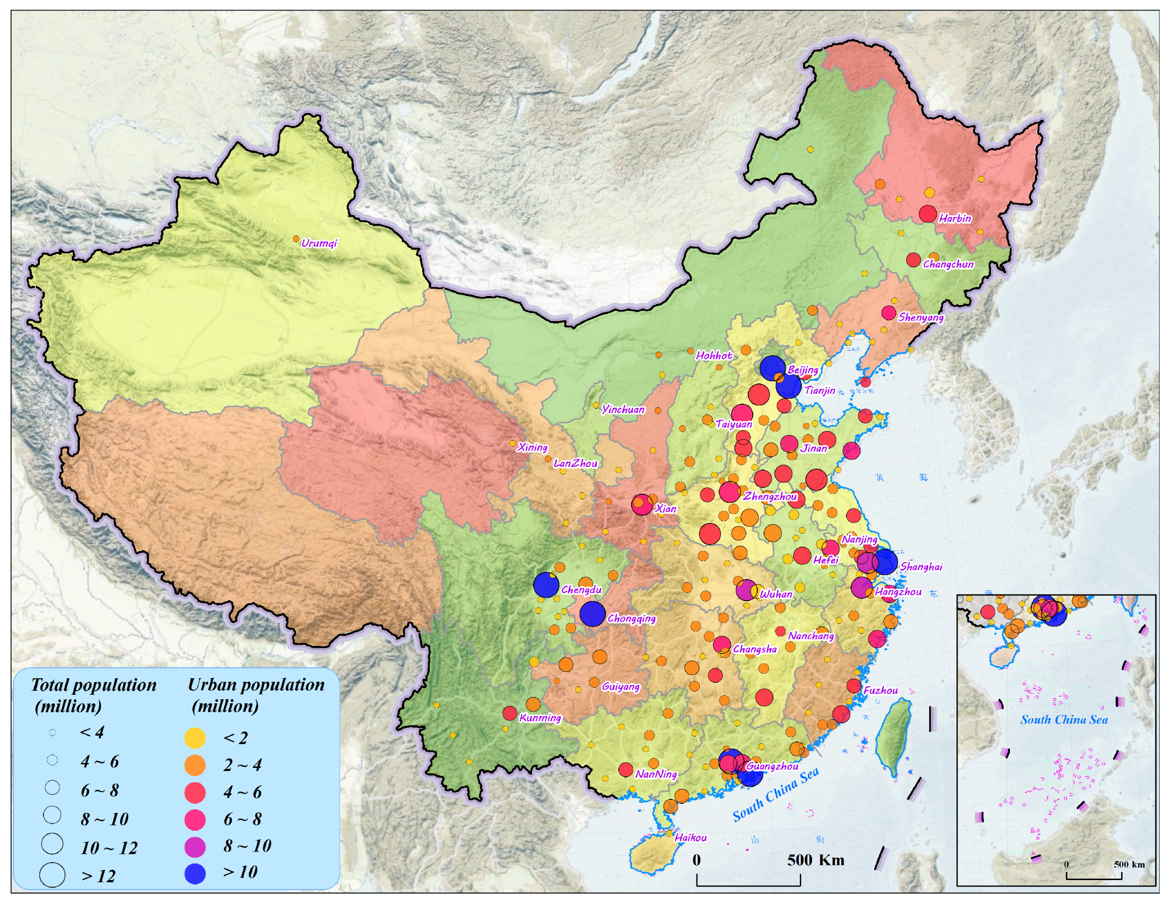
Figure 1. The 234 sample cities with total population larger than 2 million in 2019 in China.
Remotesensing 15 01426 g001
Figure 2. Overview of the technique flow in this study.
Remotesensing 15 01426 g002
Figure 3. Illustration of urban centers (axes) and concentric rings in monocentric cities (a), nonlinear polycentric cities (b), and cities with ribbon-shaped growth (c).
Remotesensing 15 01426 g003
Figure 4. (a,b) Spatiotemporal pattern of nighttime light and its changes at five-year intervals during 1992–2018 in a representative city, Wuhan.
Remotesensing 15 01426 g004
Figure 5. Intensity of human activity within concentric rings of a representative city, Wuhan, when the lower limit of DN value to extract human activities is set to 1 and 30 (the interval of time is 5 years, i.e., Δ t = 5 ) .
Remotesensing 15 01426 g005
Figure 6. Wave of spatiotemporal variations in different levels of human activities in Wuhan from 1992 to 2018 when the time intervals are fixed as 5 years and the D N m i n parameter varies from 1 to 50 (the lower and upper limit of the y-axis in subplots is 0 and 1, respectively).
Remotesensing 15 01426 g006
Figure 7. Wave of spatiotemporal variations in intensity of human activities in a typical city, Wuhan, from 1992 to 2018, when D N m i n = 30 and the time interval varies from 1 to 9 years with increments of 2 years.
Remotesensing 15 01426 g007
Figure 8. Goodness of fit (R2) of different bell-like functions when fitting the empirical waves of variations in human activity intensity observed during 1992 and 2018, with the lower limit of DN values varying from 1 to 50 (with an increase of 10) and the time interval varying from 1 year to 9 years (with an increase of 2 years). The red point indicates the mean value of R2. Note that if a function fails in fitting an empirical wave, then it was excluded from the boxplot.
Remotesensing 15 01426 g008
Figure 9. Goodness of fit of the Gaussian model for fitting spatiotemporal variations in intensity of urban-related human activities observed in the 234 sample cities between 1992 and 2018, with lower limit of DN values set to 30 and interval of time set to 5 years. (The x-axis of the central plot indicates the 234 cities in ascending order of their urban population from left to right, and the y-axis indicates the years (1992–2018) from top to bottom in an ascending order. The subplot at the top indicates the average R2 of the fitted Gaussian model of each city, and the subplot on the right indicates the average R2 of each time interval.)
Remotesensing 15 01426 g009
Figure 10. Parameters of Gaussian models fitted for spatiotemporal variations in intensity of urban-related human activities observed in the 234 sample cities between 1992 and 2018, with lower limit of DN values set to 30 and interval of time set to 5 years.
Remotesensing 15 01426 g010
Figure 11. Degree of consistency (R2) between the observed and deduced patterns of total intensity of human activities of different levels, with the time intervals ranging from 1 to 9 years.
Remotesensing 15 01426 g011
Figure 12. Observed and deduced patterns for urban-related human activities in 10 typical cities of different sizes (the value in the upper right corner indicates the R2).
Remotesensing 15 01426 g012
Table 1. Overview of datasets used in this study.
DataSourceSpace-Time ResolutionDescription
Nighttime nightA harmonized global nighttime light dataset produced by Li et al. [40] which can be downloaded from https://doi.org/10.6084/m9.figshare.9828827.v2 on 19 September 2022Spatial resolution: 30 arc-seconds (about 1 km near the equator)
Time resolution: 1 year
Time span: 1992–2018
These NTL data record the DN values, ranging from 0 to 63, to indicate the intensity of city light at night.
Impervious surfaceA global-scale impervious surface dataset mapped in 30 m resolution by Huang et al. [42] which is freely available at irsip.whu.edu.cn/resources/resources_en_v2.php on 17 September 2022Spatial resolution: 30 m
Time resolution: 1 year
Time span: 1972–2019
We use impervious surface data from 2018 to help identify urban centers.
Extent of functional urban areasA global urban boundaries dataset mapped from the global artificial impervious area (GAIA) data by Li et al. [43], accessed at http://data.ess.tsinghua.edu.cn on 15 September 2022Spatial resolution: vector
Time resolution: 1 year
Time span: 1990, 1995, 2000, 2005, 2010, 2015, and 2018
We use urban boundaries of each city in 2018 as auxiliary data to locate urban centers.
Total and urban populationStatistical yearbookTime resolution: 1 year
Time span: 2019
The population dataset was used to select and group the sample cities.
Urban planning mapsOfficial websites of the Bureau of Natural Resources——Auxiliary data was used to locate urban centers.
Table 2. Other functions used to fit empirical waves of variations in human activity intensity.
Name of
Function
Basic Form in
Literature
Derivative Form Used in This StudyDescription of Parameters
Gaussian function f ( x ) = a × e ( x b ) 2 2 c 2 f ( x ) = a × e ( x b ) 2 2 c 2 + d Parameter a is the amplitude of the Gaussian function; b and c are the mean and standard deviation, respectively. d is a constant parameter that offsets the function along the y-axis ( a > 0 ,   c > 0 , d > 0 ).
Quadratic
exponential function
f ( x ) = a × e b x + c x 2 f ( x ) = a × e b x + c x 2 + d Parameter a impacts the height of the function curve. Parameter b and c determine the central location (i.e., b / 2 c ) and the width of the function curve, respectively. Parameter d offsets the function along the y-axis ( a > 0 ,   d > 0 ).
Linear gamma function f ( x ) = a × e ( b x ) × x k f ( x ) = a × e ( b x ) × x k + d Parameter a impacts the height of function curve. Parameter b and k determine the central location (i.e., b / k ) of the function curve. Parameter d offsets the function along the y-axis ( a > 0 ,   b < 0 ,   k > 0 , d > 0 ).
Lognormal
function
f ( x ) = a × e ( ln ( x ) b ) 2 2 c 2 f ( x ) = a × e ( ln ( x ) b ) 2 2 c 2 + d Parameter a is the amplitude of the lognormal function; b and c are the mean and standard deviation, respectively. d is a constant parameter that offsets the lognormal function along the y-axis ( a > 0 ,   c > 0 , d > 0 , x > 0 ).
Fuzzy logic function f ( x ) = 1 1 + | x b c | 2 k f ( x ) = a × 1 1 + | x b c | 2 k + d Parameter a is the height of fuzzy logic function; b and c determine the center and width of the function, respectively; k (together with c) determines the slope ( k / 2 c ) of the curve. d is a constant parameter that offsets the function along the y-axis ( a > 0 ,   c > 0 , d > 0 , k > 0 ).
Logistic function f ( x ) = e x ( 1 + e x ) 2 f ( x ) = a × e x b c ( 1 + e x b c ) 2 + d Parameter a impacts the amplitude of the function; b and c determine the central location and the width of the function curve, respectively. Parameter d offsets the function along the y-axis ( a > 0 ,   c > 0 , d > 0 ).
Gudermannian function f ( x ) = 2 e x + e x f ( x ) = a e x b c + e x b c + d
Disclaimer/Publisher’s Note: The statements, opinions and data contained in all publications are solely those of the individual author(s) and contributor(s) and not of MDPI and/or the editor(s). MDPI and/or the editor(s) disclaim responsibility for any injury to people or property resulting from any ideas, methods, instructions or products referred to in the content.