Abstract
Against the background of the ongoing atmospheric warming, the glacial lakes that are nourished and expanded in High Mountain Asia pose growing risks of glacial lake outburst floods (GLOFs) hazards and increasing threats to the downstream areas. Effectively extracting the area and consistently monitoring the dynamics of these lakes are of great significance in predicting and preventing GLOF events. To automatically extract the lake areas, many deep learning (DL) methods capable of capturing the multi-level features of lakes have been proposed in segmentation and classification tasks. However, the portability of these supervised DL methods need to be improved in order to be directly applied to different data sources, as they require laborious effort to collect the labeled lake masks. In this work, we proposed a simple glacial lake extraction model (SimGL) via weakly-supervised contrastive learning to extend and improve the extraction performances in cases that lack the labeled lake masks. In SimGL, a Siamese network was employed to learn similar objects by maximizing the similarity between the input image and its augmentations. Then, a simple Normalized Difference Water Index (NDWI) map was provided as the location cue instead of the labeled lake masks to constrain the model to capture the representations related to the glacial lakes and the segmentations to coincide with the true lake areas. Finally, the experimental results of the glacial lake extraction on the 1540 Landsat-8 image patches showed that our approach, SimGL, offers a competitive effort with some supervised methods (such as Random Forest) and outperforms other unsupervised image segmentation methods in cases that lack true image labels.
1. Introduction
Glacial lakes are of considerable interest due to their sensitivity to the ongoing climate changes and threatening outburst risks to downstream communities in High Mountain Asia [1,2,3]. As a typical component of water resources, glacial lakes are positioned in glacierized regions and fed by melting glaciers. As they are adversely impacted by glacier shrinkage and seasonal climate variation, glacial lakes have grown rapidly in terms of both number and area [1,2,3,4,5], especially in recent decades, concomitant with the increases in glacier-related hazards such as glacial lake outburst floods (GLOFs) [6,7]. To monitor the dynamics of lakes and give forewarning of GLOFs, the automatic and accurate extraction of glacial lakes from remotely sensed images is a prerequisite for the fast evaluation of these outlying lakes.
Many approaches have been explored by coupling two or more types of optical imagery, including the digital elevation model (DEM), synthetic aperture radar (SAR), thermal infrared image and satellite altimetry for glacial lake extraction. For example, Li et al. [8] and Song et al. [9] employed the Normalized Difference Water Index (NDWI) to highlight the lake information and extracted this information by leveraging a local threshold derived from bimodal histograms in the buffer zone of each potential lake area. Gardelle et al. [10] combined green, Near Infrared (NIR) and Short Wave Infrared (SWIR) bands to map the frozen glacial lakes or lakes with floating ice. Wangchuk et al. [11] collected a lot of pixels from the lake area and the non-lake area, and they gave a category for each pixel according to the patterns of the glacial lakes in high-dimensional space learning from the random forest. Shen et al. [12] and Li et al. [13] conducted an object-oriented method to identify the potential lake areas and refine the final lake area by a pre-defined water extraction decision ruleset. Zhao et al. [14] integrated the advantage of threshold segmentation and a simplified active contour model to extract small glacial lakes. Mitkari et al. [15] proposed an object-based image analysis (OBIA) method for mapping small supraglacial lakes from high spatial resolution data of LISS-IV. Zhang et al. [16] used a phase-congruency-based detector on the C-band of SAR images to extract the area of glacial lakes according to their outline and texture. However, many influencing factors, including the physical properties of lakes (glacial lakes of differing size, turbidity, depth and coloring) and complicated environmental conditions (such as shadows from mountains and clouds and melting glaciers) [2,3,8,9], still pose challenges to large-scale glacial lake extraction. In particular, the different intrinsic physical properties cause the lake to show varying spectral responses, and the extrinsic geomorphic factors always show similar spectral values to glacial lakes; these cause difficulties in differentiating glacial lakes against diverse factors in remotely sensed images. Although they possess good performance and high accuracy, these traditional methods still require extensive pre- or post-processing to determine the optimal segmentation parameters and to eliminate the effects from these factors.
Recently, with the advancements in the DL model, many tasks in terms of classification, segmentation and object detection have achieved great signs of progress as the DL method can capture the high-level features of objects and give final decisions based on these feature patterns. Some DL models have also been successfully applied in glacial lake extraction. For example, Kaushik et al. [17] used a Deep Convolutional Neural Network (DCNN) to automatically map the glacial lakes from multisource remote sensing (RS) data; Qayyum et al. [18] and Wu et al. [19] employed a U-net model to extract the contours of glacial lakes; Thati et al. [20] utilized a V-net model to segment the water and non-water bodies from satellite imagery; and Zhao et al. [21] proposed a GAN-based architecture for glacial lake mapping. These five DL-based models utilized convolution operations to capture the high-level spatial features and skip connections to integrate the features at different scales, so that the model learns the patterns of glacial lakes and greatly improve the accuracy of the glacial lake extraction. Although their performance far exceeds that of the traditional methods, and without the use of any other ancillary data (such as the Digital Elevation Model (DEM) [18,19,20,21]) and post-processing work, they require a lot of effort to prepare the training labels. These supervised DL methods limit the applicability of the glacial lake extraction method to different data modalities.
To avoid assembling such large annotated image labels and to extend the model training for downstream tasks, some works explore the unsupervised (without labeled data) or semi-supervised (with few labels) representation methods and obtain notable progress [22,23,24,25,26,27,28,29,30]. As a conspicuous breakthrough in unsupervised learning, contrastive representation learning is based on the intuition that the same object in various transformations of an image (multi-view, color change, rotation, blurring) should have similar representations, whilst being dissimilar to the representations of other objects. Several contrastive learning works, including SimCLR [26], MoCo [27], SwAV [28], BYOL [29] and Simsiam [30], use a Siamese network to find the valuable representation by maximizing the similarity between the input image and its augmentations. SimCLR [26] and MoCo [27] provided a training strategy without a memory bank; SwAV [28] applied the online clustering mechanism to the Siamese network; BYOL [29] designed an asynchronous momentum encoder to solve the issues of constructing negative pairs; Simsiam [30] proved that a contrastive network learns the meaningful representations without inputs of negative sample pairs, momentum encoders and large batches in the training stage. These encouraged us to explore the unsupervised DL methods for glacial lake extraction. As seen in Figure 1, the traditional DL methods require the input of an image and a true mask of the glacial lake, which prevents the model from capturing the lake features and learning the lake patterns. Contrastive learning is to find the lake areas by transforming the input image and generalizing the features of the lakes.
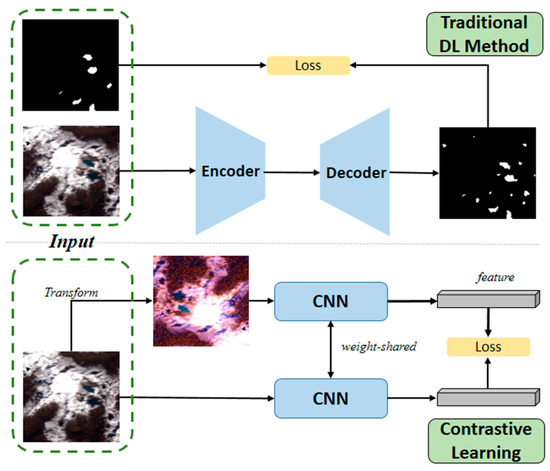
Figure 1.
Different inputs and training strategies in contrastive learning and traditional deep learning (DL) methods in glacial lake mapping. DL methods always need to input labeled lake masks to construct the loss function, while contrastive learning calculates the loss function between the input image only and its augmentations.
In this work, we proposed a simple glacial lake extraction network (SimGL) via weakly-supervised contrastive learning. In our design, a remote sensing image is the only input. Zhang et al. [31] evaluated the extraction performance of glacial lakes using 23 classical spectral features and concluded that the NDWI has great potential in glacial lake mapping; therefore, we employ a strict NDWI map segmenting with tight thresholds to provide rough location cues of glacial lakes and as a pseudo label. Inspired by contrastive learning works [26,27,28,29,30], a Siamese network cascading a prediction head is introduced to learn similar representations and sort out the same objects. Our loss function consisted of two parts: a contrastive loss in the Siamese network to constrain the segment processing to learn similar representations; and a location loss between the segmentations and NDWI maps to capture the precise boundaries of the glacial lakes. The impressive evaluating results of the glacial lake mapping on the Landsat-8 imagery also demonstrate that our model can obtain a competitive performance with some supervised methods and shows great potential in learning the patterns of glacial lakes without labeling data.
We summarize the contributions of our work threefold:
- We proposed a simple yet effective glacial lake extraction model, SimGL, which effectively learns lake representations from unlabeled RS images via contrastive learning in the training stage.
- We further introduced the NDWI map into our model to provide location cues of the glacial lakes and proposed a location loss to encourage the segmentations to coincide with the true glacial lake boundaries.
- We evaluated our model SimGL using four metrics and compared the segmentation performance with other glacial lake mapping methods on the Landsat-8 imagery. The results demonstrate that our model SimGL surpasses other unsupervised methods and narrows the performance difference with supervised DL methods.
2. Methodology
In this section, we introduce the architecture of SimGL (as shown in Figure 2) and explain the loss function, in which the components are detailed in the following subsection. From Figure 2, our model consists of two parts: (1) an NDWI map, regarded as a pseudo label, provides the lake location cues and penalizes the network for segmenting the lake masks; (2) a Siamese network learns the meaningful representations of objects by maximizing the similarity between two inputs. Note that we only use some simple strategies to provide the location cues of the lakes. Neither image label supervision nor a sophisticated structure (such as salient object detection) is involved in the model training.
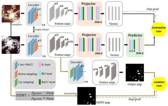
Figure 2.
The architecture of the proposed SimGL. It consists of two parts: one takes the RS image and its augmentations as input pairs for a Siamese network, which generates a set of feature maps at different scales. Then applying the prediction layer on projected features from one branch to predict the transform features from another branch, and we use a contrastive loss to measure the similarity between the two features. Another part only takes the RS image as input, then a location loss was calculated between the output map (generated by decoding the multi-scale features) and location cues (generated by thresholding the NDWI map) to constrain the segmentation results.
2.1. Preliminaries
Given an RS image with height h, width w and channel c, we aim to find the network designs f that detect the lake segmentation mask from the input image x using a weakly-supervised training strategy. If any location in image x is denoted by u, this process can be modeled as ; where θ is the parameters of the network, our model uses two loss terms to learn the segmentation parameters − contrastive loss and location loss.
2.2. Weakly Location Cues from NDWI Map
Benefiting from its simple calculation and convenient application, the Water Index (WI) is the most frequently used method for locating the lake area. Among the WIs, NDWI has been widely applied in glacial lake mapping due to its great superiority in eliminating the effects of confounding factors with glacial lakes, such as mountain shadows and melting glaciers [8,9]. Here, the NDWI was defined by [32]:
where and represent the Top-of-Atmosphere (TOA) reflectance values in the green and NIR bands measured by sensors, respectively.
The NDWI map contains the position cues of the glacial lakes. Most previous research has set a threshold in the range of 0.0 to 0.4 to segment glacial lake areas in the NDWI map. Although a low threshold can segment the glacial lake pixels as much as possible, some other pixels that have similar spectral feature values with glacial lakes will also be retained. We aim to find the accurate lake pixels as a pseudo label to provide the lake information to the model; a high or tight threshold should segment the glacial lake pixels only and avoid the effects from any other object pixels. Therefore, we set a tight threshold T on the NDWI map to obtain the lake binary mask B, where we assign the value 0 for the background and 1 for the glacial lake. This step is called weak localization and is illustrated in the brown part in Figure 2. With a tight threshold, all non-lake pixels and some lake pixels confused with the background are removed, leaving only the glacial lake areas in binary masks. Although the lake areas may not be complete and precise enough in this mask, the mask is helpful in guiding the network to seek objects that are similar to the glacial lakes. To describe the similarity between the masks and segmentation results, we introduce a location loss, which is defined as follows:
In the location loss, there are many existing ways to generate the binary mask B, such as salient object detection (SOD) [33,34], whereas glacial lakes are too small to be identified by SOD. Thus, we use a simple WI to localize the glacial lakes.
2.3. Contrastive Semantic Segmentation
In our Siamese network, we use a weight-shared encoder, which contains four down-sampling blocks, to capture similar objects from two inputs at different scales. The multi-scale feature maps are represented by q = [q1, q2, q3, q4]. To measure the similarity of two sets of feature maps, the feature maps are input to a projector to output the embedding vectors [29,31]. A vector of an image should be predictive of the vector of the transformed image [29]; therefore, we employ a predictor p to transform one vector and match it to the vector from another branch (as “predictor” in Figure 2) [29,31]. Here, we use the negative cosine similarity to measure their matching score:
where q’ denotes the feature map encoded from the transformed images x’. Following the work [31], we use a stop-gradient operation (see “stop-grad” in Figure 2) to avoid the model subjecting to model collapse. Therefore, the Formula (3) can be modified as:
This indicates that the q’ was regarded as a constant in Formula (4). Following [29,31], two symmetrical components have consisted of our contrastive loss:
Overall, our model was trained with a composition of two loss functions:
Here, the λ is the hyper-parameter balancing two loss terms. The location loss acquired from an input image and the NDWI map provides a piece of weakly supervised lake information, while the contrastive loss, as in Formula (5), forces the network to contrast the similarities between the inputs and their augmentations and penalizes the network for seeking the feature maps of the same objects.
2.4. Image Augmentation
We defined seven ways to generate the augmentations of multi-band RS images.
- (1)
- Color jitter. We use color jitter with {brightness, contrast, saturation, hue} strength of {0.4, 0.4, 0.4, 0.2} for the RGB bands of the RS images as the hue is only well-defined for the RGB data.
- (2)
- Gray scaling. We use gray scaling to remove the color information and represent each pixel only by its intensity.
- (3)
- Flipping. We randomly flip an image along with a horizontal or vertical location.
- (4)
- Rotating. We randomly rotate an image by an angle in the set of {90°, 180°, 270°}.
- (5)
- Blurring. The images are blurred with the Gaussian kernel; here, the kernel size is 3 × 3 and the other parameters maintain the default values.
- (6)
- Random area erasing. We randomly masked some pixels (less than 1% image size) with 0 to erase the spectral information.
- (7)
- Noise addition. We add the Gaussian noise to the image.
An example of transforming a glacial lake image in different ways is shown in Figure 3. These transformations perturbed the spectral features or spatial features, which is crucial to enhance the robustness of the model training.
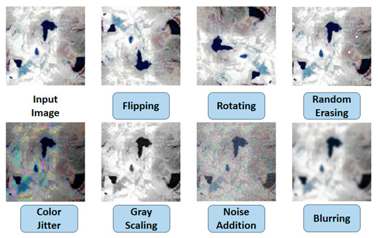
Figure 3.
Different ways to generate the augmentations of multi-band RS images.
2.5. Detailed Network Architecture
Overall, the components of our models included (see Figure 2):
- Encoder and decoder: The encoder and decoder are the same as the structures in the U-net. We use the encoder to capture the feature maps at different scales from the input image and the decoder to reconstruct the segmentation results of the lakes from the feature maps. In our model, each selected feature map is from the results before the down-sampling operation.
- Projector: The projector has three fully-connected (fc) layers and batch normalization (BN) layers, and the first two layers are activated by ReLU. The output of the projector is a 2048-d vector.
- Predictor: The predictor has two fc layers. The first is connected to a BN and a ReLU layer, and the last is without any other operations. The output dimension is 2048-d, while in hidden layers, it was set as 512-d.
3. Experiment Results
In this section, we give a detailed study on validating the SimGL and comparing our model with the state-of-the-art models.
3.1. Dataset and Evaluation Metrics
Dataset: Landsat-8 OLI images have a suitable spatial resolution (30 m) and moderate revisiting period (16 days), benefiting the glacial lake investigation over a large-scale region. We collected 103 Landsat-8 images (all images were acquired in the autumn of 2016 as the boundaries of the glacial lakes are clearer in this period), and then randomly cropped 256 × 256 × 7 image patches from these images. Only the patch containing lake pixels greater than an 1% area of the patch is kept. To make the corresponding lake labels, we first converted the High Mountain Asian Glacial Lake Invention dataset (Hi-MAG) [1] in 2016 into a raster file with 30 m spatial resolution. Secondly, we cropped the raster file according to geographical coordinates of patches and made them consistent in range. Finally, our dataset contains 1540 image patches and 1540 corresponding labels. In our experiments, we split the dataset into 70% for training, 20% for validation and 10% for testing. More details of our dataset are summarized in Table 1.

Table 1.
Details of our dataset.
Evaluation metric: in our study, we use four metrics to evaluate the segmentation effects on glacial lakes: Precision (P), Recall (R), F1 Score (F1) and Intersection over Union (IoU). They are defined following [21]:
P = correctly extracted water pixels/all extracted pixels;
R = correctly extracted water pixels/all water pixels;
F1 = 2 × P × R / (P + R);
IoU = (extracted water pixels ∩ true water pixels)/(extracted water pixels ∪ true water pixels).
3.2. Implementation Details
All of the experiments were implemented using Tensorflow 1.14 on the Python 3.7 platform with one GTX 1660 Ti GPU (6 GB GPU memory). For the hyper parameters, we followed the conventions [31] to set the initial learning rate as 0.005. Then, it was scheduled following a cosine decay policy, with a decay rate of 0.0001. For training, we set the loss coefficient λ as 10. Our model SimGL was trained by Adam optimizer and the training 100 epochs with a batch size of 8.
3.3. Diagnostic Experiments
Coefficient λ in joint loss: The coefficient λ balances the influence of two types of losses, and we give the segment performance for the values of λ changed from 10−4 to 104, as shown in Figure 4. Obviously, the optimal segmentation performance of the F1 score and IoU occurred as the λ reached 10. Therefore, we set the λ to 10 as it has good effects on balancing two loss terms.
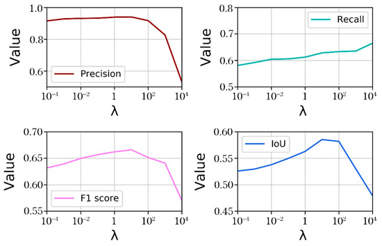
Figure 4.
The effects of coefficient λ on the segmentation results. The horizontal axis is the range of λ from 10−4 to 104, and the vertical axis reflects the value of each metric. Obviously, optimal segmentation performance of F1 and IoU occurred as the λ reached 10.
Loss term ablation: To prove whether using the NDWI only or the contrastive module only is enough for glacial lake mapping, we explored the model effects when part of the model was ablated; namely, only one type of loss used or both two loss terms used. The loss term ablation results are shown in Table 2. As our Landsat patches are similar in content, including glacial lakes, glaciers, shadows, etc., these high-frequency objects will also be extracted with the glacial lakes when using contrast learning only, which caused a low F1 score (0.1356) and IoU (0.1083) in the loss ablation results. Although the model can yield good results using location loss only, the location cues provided by the NDWI map were not accurate enough to true lake boundaries. Thus, our model SimGL combined the advantages of two loss terms and further improved the segmentation results.
Table 2.
Ablation results of using different loss terms.
Water Index and thresholds: Many WIs are designed to highlight the lake information; some of them include NDWI [32], MNDWI [35] and MI [36]. They are always combined with threshold segmentation to segment the WI maps to the lake binary masks. In our model, the use of a rough lake location map as a pseudo label is required to directly guide the segmentations to be more accurate and less contaminated by the background. In most glacial lake mapping research, the thresholds of these three WIs range between 0.0 and 0.4 [1,8,9]. Therefore, we explore how the segment performance and their evaluation metrics are affected when setting gradually tight thresholds in a broad range of [−0.1, 0.8], as shown in Figure 5.
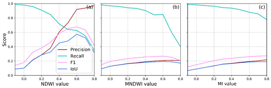
Figure 5.
The effects between thresholds and evaluation metrics on the NDWI, MNDWI and MI, respectively. (a) Threshold ablation for NDWI. We set 0.6 of the NDWI threshold for further experiments as it can balance the lake information and noise information. (b) Threshold ablation for MNDWI. The best threshold of MNDWI should be 0.6 for providing pseudo lake masks. (c) Threshold ablation for MI. The best threshold of MNDWI should be 0.7 for providing pseudo lake masks.
Specifically, from Figure 5, the F1 and IoU progressively increase when we set the threshold more tightly to 0.6 in three WIs, but decrease when setting the threshold to a high value (great than 0.7). For example, when we set the NDWI threshold as 0.6, our model will achieve an astonishing performance as it has the highest Precision, F1 and IoU (see Figure 5a). Similarly, they are 0.6 for MNDWI (see Figure 5b) and 0.7 for MI (see Figure 5c). The glacial lake pixels always show high WI values, as well as some pixels from melting glaciers and mountain shadows; thus, a tight threshold can filter out the more glacial lake pixels, but the noise pixels are extracted if we use a loose threshold.
Moreover, we further visualized the results of SimGL when setting different thresholds on NDWI, MNDWI and MI, as shown in Figure 6.
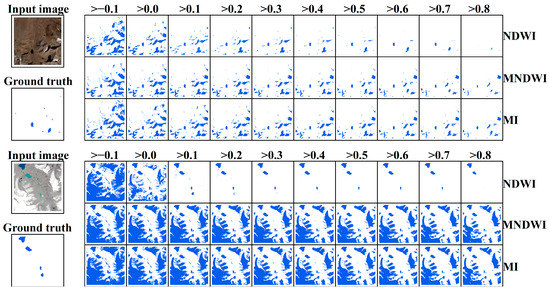
Figure 6.
Two visualized samples of SimGL when setting different thresholds and WIs in the pseudo label generation stage. The blue area is lakes extracted by SimGL. From visualizations, the model output is closest to the ground truth when we set the threshold in the range of [0.5, 0.7] on NDWI.
As shown in Figure 6, the experimental results were heavily contaminated by the glaciers when using MDNWI and MI. This also proved that the NDWI is more accurate in generating lake masks, especially in glacierized regions. In addition, almost all of the extracted pixels belonged to glacial lakes when the threshold of NDWI was set to be greater than 0.5, indicating that a tight threshold will facilitate the model to learn the lake’s information more accurately.
Types of image augmentations: Seven methods are defined for transforming an image in our experiments. We further divide them into two groups to explore the influence of each type and group. One contains {color jitter, gray scaling, blurring, random area erasing and noise addition}, which will change the spectral distribution of an image. The other one uses a {flipping and rotating} operation to change the location of each pixel. Table 3 shows the evaluation metrics in the case of employing one type of group transformation method. Each type in a group is processed with an applying probability of 0.6 in the evolution experiments.
Table 3.
Evolution results of different types of image transformation.
From Table 3, we found that the flipping operation obtained the highest F1 and IoU scores, and the lowest F1 and IoU were scored by random area erasing. Thus, we considered giving a high probability to some important transformations; finally, we set applying probabilities of {0.7, 0.6, 0.8, 0.7, 0.5, 0.5, 0.5} to the transformations of {color jitter, gray scaling, flipping, rotating, blurring, random area erasing and noise addition}.
3.4. Comparison with the State-of-the-Arts
In this subsection, we compare our model with other widely used mapping methods, including some supervised and unsupervised methods:
- NDWI: WI is the most simple and widely used method in glacial lake mapping, including in NDWI [32] and MNDWI [35]. Among these indexes, the NDWI is the most feasible way to highlight the lake information and suppress the background information [31]. To test the segmentation performance of using NDWI only, we set the segmentation threshold to 0.6, the same as we used in our model.
- Global–local iterative segmentation algorithm (GLSeg) [8,9]: The GLSeg includes two hierarchical image segmentation stages. First, segment the NDWI map to delineate the potential lake areas using a global threshold. Second, calculate the local threshold to determine the extent of each potential lake within a buffer zone of the lake. Moreover, the auxiliary data (such as DEM) are introduced to filter the noise pixels with similar NDWI values with the glacial lakes. For fairness, we only use the RS imagery as the input, and the parameters are set following [8,9]. We set NDWI > 0.1, NIR < 0.15 and SWIR < 0.05 in the global segmentation stage and the local threshold was computed according to the mean and variance of the lake and background pixels.
- C-V model (C-V) [14,37]: as a region-based segmentation method, the C-V model shows great anti-noise ability, which improves the segmentation accuracy in the homogenous areas of glacial lakes and avoids the influences of individual noise pixels from the surroundings. The C-V model employs an active curve to separate the image into inner parts and outer parts and uses an energy function to evaluate the segment results. When the energy function reaches an optimal state, the curve will converge to the true lake boundaries. The parameters are set following [14,37].
- Random Forest classification (RF) [11]: RF has good robustness and generalization in classification tasks because of its random sampling operations on the input data and features in each decision tree. For the RF training, we set 1000 trees to vote whether a pixel belongs to the glacial lake or not, and our training set includes 93,431 glacial lake samples and 93,431 non-lake samples, each of which has seven band values and a class label.
- U-net [18,20,38]: U-net is the first DL model for glacial lake segmentation. It learns the pattern of glacial lakes in order to eliminate the dependence on the auxiliary data (such as using DEM to remove the mountain shadows). U-net contains four pairs of encoder and decoder units, and a skip connection is employed to concatenate feature maps from different scales and capture more details of the lake boundaries. Finally, the output mask is the segmentation results. We set the parameters to be the same as [18].
- GAN-GL [21]: GAN-GL uses a zero-sum game between a generator and a discriminator to find the stable state, and a water attention module is also introduced to accelerate the convergence process. This GAN-based method can delineate the glacial lake boundaries more easily, without any distribution assumptions.
We evaluated the glacial lake extraction effects of these segmentation methods on the validation dataset, and the results are shown in Table 4. Evidently, the segmentation effects of the unsupervised segmentation methods (NDWI, GLseg, C-V) are significantly lower than that of the supervised methods (RF, U-net, GAN-GL) by comparing the F1 score and IoU. As for comparing these unsupervised methods, our model has yielded the best performance and even shows competitive efforts to the supervised classification method (RF).
Table 4.
Evaluation results of segmentation methods weather it involves label or threshold.
4. Discussion
In this section, we discuss the benefit and defects of our model SimGL, and its applicability to other sensors.
4.1. Visualization of Comparisons
Figure 7 shows the visualization results of the glacial lake extraction performances. By comparing the results from other glacial lake extraction methods, our SimGL shows several potential improvements. First, the results from the pixel-based methods (NDWI, GLseg, and RF) demonstrated that they are prone to producing noises or individual pixels (see Figure 7a,c), which may come from mountain shadows, melting glaciers and floating ice, while our model SimGL utilized the convolution operation to capture the spatial features of glacial lakes, showing that it had an excellent anti-noise ability. Second, compared to the supervised method RF, our model SimGL shows good effects in extracting lakes with floating ice or frozen surface (see Figure 7b,d,f). Considering the three unsupervised glacial lake extraction methods (the NDWI, the C-V model and the GLseg model), some small lakes were detected by the C-V model and the GLseg model, but not extracted by NDWI. As a low global threshold of 0.1 was set in C-V and GLseg, some small lakes that are easily confused with background (they always have a low NDWI value) are discriminated. This means that the location cues provided by the NDWI map are not accurate enough for the glacial lake areas, but our model SimGL extracted more lake pixels than when employing NDWI only (see Figure 7f), which also illustrated that our model SimGL could learn the patterns of glacial lakes from limited lake information.
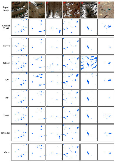
Figure 7.
Visualization of segmentation results of the glacial lake by employing different methods. Extracted lakes are marked in blue. (a–f) are six regions of glacial lakes developed in different surroundings.
Despite the supervised DL model (U-net and GAN-GL) designing an automatic scheme to segment glacial lakes and obtaining an exceptional performance, these methods are still inevitable to prepare a large number of training images and labels. Therefore, our method SimGL provides a new scheme to segment the glacial lakes in cases of lacking true lake labels in large-scale areas.
4.2. Applicability to Different Sensors
To determine the generalizability and robustness of the model, we conducted our model on four types of data: the Landsat-5 Thematic Mapper (TM), Landsat-7 Enhanced Thematic Mapper Plus (ETM+), Landsat-8 Operational Land Imager (OLI) and Sentinel-2 Multi-Spectral imager (MSI). Here, the Landsat-8 OLI has a higher radiometric resolution (16 bits) than its predecessors (eight bits in Landsat-5 TM and Landsat-7 ETM+), representing an abundant color of information in the image. In terms of the Sentinel-2A MSI imagery, although it has a high cloud cover of 66.07%, fortunately the region where the glacial lake is nourished is cloud-free, and the lake boundary is clear enough to implement segmentation experiments. Moreover, considering that the Sentinel-2A MSI imagery has 13 bands with different spatial resolutions, we finally stacked the layers of band 2/3/4/8 (corresponding to blue/green/red/NIR bands) to an image file as they all have 10 m spatial resolution. The detailed information of the four images is listed in Table 5.
Table 5.
Detailed information of images from four different sensors.
The model configurations remained as those described in Section 3.2. The training dataset was the abovementioned 1540 Landsat-8 OLI image patches. However, the image bands of the sensor TM, ETM+ and MSI do not correspond exactly to that of the sensor OLI. Therefore, we selected the bands contained in both the testing image and the Landsat-8 OLI image during the training stage. Specifically, we trained the model with the blue/green/red/NIR/SWIR1 bands of the OLI image for testing the TM and ETM+ images, and then re-trained the model with the blue/green/red/NIR bands of the OLI image for testing the MSI image. Despite these images being varied in their bit depth and DN value ranges, the object reflectance should remain consistent, even in different data. Thus, we automatically convert the DN value of the Landsat-8 OLI images to the TOA map before the model training, and the conversion parameter values can be queried in the head file. Only the training data and testing data are reflectivity products; the model can predict the testing image according to the features learned from the training data.
Finally, the experimental results of the different sensors are shown in Figure 8. From the first row and third row in Figure 8, the glacial lake areas extracted by our model SimGL are very close to the true lake areas and without noise interference, even if different RS images are used for the experiment, which also indicates that our model has good applicability and can be easily applied to the other RS image.
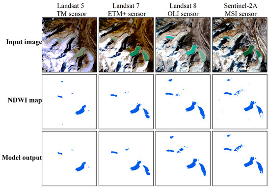
Figure 8.
The visualization results of our model SimGL conducting on four different RS images. The blue areas are extracted lakes. The first row shows the RS images from Landsat-5 TM, Landsat-7 ETM+, Landsat-8 OLI and Sentinel-2A. The second row is the segmentation results by thresholding the NDWI map with a value of 0.6, the pixels great than this value will be marked as lake pixels. The third row is the testing results using our model SimGL.
4.3. Possibility in Monitoring GLOF Events
All the glacial lake extraction methods are finally expected to conveniently monitor and find potentially dangerous lakes on a large scale, then give early warning for some dangerous lakes under long-term observations by remote sensing. Recently, some works have attempted to extract glacial lakes at different periods and analyze them to identify the lakes with a high outburst risk. For example, Ahmed et al. [39] used a simple weighted index on high-resolution satellite data for glacial lake mapping and change detection analysis, and 21 glacial lakes were marked as potentially dangerous lakes in the upper Jhelum basin, Kashmir Himalaya, India; Nie et al. [40] extracted the glacial lake extent in 1990, 2000, 2005 and 2010, employing an object-oriented segmentation method and manual inspection, ultimately identifying 118 lakes as potential vulnerable lakes in Himalaya; Shrestha et al. [41] delineated the glacial lake boundary using NDWI in the years 1977, 1990, 2000 and 2010 in the Koshi basin of Himalaya and found 42 rapidly growing glacial lakes that should be paid more attention in terms of GLOF.
These works use simple segmentation methods (such as NDWI) to extract glacial lakes at a regional scale and identify the dangerous ones through the comparative analysis of lake areas in different periods. While our model SimGL has better applicability to RS sensors and a better segmentation performance, which greatly reduces the pre- and post-processing work in the glacial lake extraction. In the future, the temporal mapping of glacial lake areas using our model, as well as investigating the lakes with high expansion rates, is imperative for recognizing the dangerous lakes and giving early warning of GLOF events.
4.4. Impaction of Locaton Cues
Owing to the similar contents of the images in the dataset, they always contain objects such as glaciers, glacial lakes, vegetation, etc.; thus, these objects are extracted with glacial lakes only using contrast learning, resulting in a low F1 score (0.1356) and IoU (0.1083) in loss term ablation. To extract glacial lakes in a case lacking true lake labels, we combined the contrastive learning and rough location cues provided by a simple Water Index. In our model, designed in Figure 2, the NDWI map provided rough location cues of glacial lakes, guiding the extraction area to coincide more with the true lake boundaries. These weak location cues are critical to the segmentation effects. Therefore, we explored how to obtain effective location cues of glacial lakes, and whether our model learned something useful with the help of this weakly-supervised information.
The model performance was first evaluated under the condition of using different Water Indexes and setting threshold values. By analyzing the results from Figure 5 and Figure 6, we can conclude that the model achieved the optimal effect when setting a threshold of 0.6 to the NDWI.
As seen in Figure 7 and Figure 8, we further visualized the results of our model SimGL and the results of using NDWI only. Three merits of our model can be deduced from the comparison of the results of the two methods: (1) The NDWI as a pixel-based method that processes each pixel by masking the pixels with a pre-defined threshold, which may contaminate the segmentations with a lot of isolated noise pixels if these isolated pixels have similar NDWI values to the lake pixels (such as in Figure 7a, many mountain shadow pixels as noise are separately extracted by NDWI). On the other hand, our model SimGL can effectively avoid the interference of noise as the model can segment the lake areas by identifying the high-level spatial features of lakes; (2) The glacial lake boundary extracted by NDWI is relatively unsmooth as the setting of a high threshold would segment an inaccurate boundary of the lakes (for example, in Figure 8, the boundary of the glacial lake was ragged when we used NDWI to map the glacial lake from Landsat-7 ETM+ imagery), but our model, as it captured and learned with the spatial features, can provide complete glacial lake areas; (3) The NDWI will fail to identify the lake pixels if they are covered by floating ice (such as the extraction results in Figure 7f and the result evaluated on Sentinel-2A MSI imagery in Figure 8). However, the SimGL can eliminate the influence of floating ice to some extent. Specifically, glacial lake areas can also be discriminated by SimGL even though the surface is covered by thin floating ice. All of these three merits suggest that our model SimGL, combining contrastive learning and rough location cues, can effectively learn the features and patterns of glacial lakes with the limited cues provided by NDWI, and give a better mapping result of glacial lakes.
5. Conclusions
In this work, we proposed a simple glacial lake extraction network (SimGL) via a weakly-supervised training strategy. This weakly-supervised DL method extends and improves the extraction performances when lacking the true labeled lake masks in the model training stage, and therefore shows good applicability to different RS data. In the SimGL, a Siamese model was utilized to capture similar objects from the input image and its augmentation via unsupervised contrastive learning. Then, a pseudo lake label provided by masking the NDWI map with a tight threshold was used to give the lake location cues and guide the segmentation. The evaluation results of the glacial lake segmentation on the 1540 Landsat-8 image patches indicated that our model outperformed the other unsupervised image segmentation methods and achieved a competitive performance with some supervised methods (such as Random Forest).
Through the comparisons with the NDWI segmentation method and the explorations of the applicability to other RS sensors data, our model shows good benefits in its anti-noise ability and applicability. In addition, although we use the NDWI map to generate the location cues to SimGL, our model can learn the features and patterns of glacial lakes with limited weakly-supervised information and segment the glacial lakes more accurately. In general, our work provides a new technology for segmenting glacial lakes from RS imagery, even without lake labels in the training stage, which significantly improves the effects of glacial lake mapping over a large-scale area.
Author Contributions
Methodology, H.Z.; validation, H.Z.; formal analysis, H.Z.; writing, H.Z. and S.W.; visualization, H.Z.; project administration, S.W. and X.L.; funding acquisition, S.W. and F.C. All authors have read and agreed to the published version of the manuscript.
Funding
This work was supported by the Strategic Priority Research Program of the Chinese Academy of Sciences (XDA19030101), the China-ASEAN Big Earth Data Platform and Applications (CADA, guikeAA20302022) and the National Key R&D Program of China (Grant No. 2018YFB0504900).
Conflicts of Interest
The authors declare no conflict of interest.
References
- Chen, F.; Zhang, M.; Guo, H.; Allen, S.; Kargel, J.S.; Haritashya, U.K.; Watson, C.S. Annual 30 m dataset for glacial lakes in High Mountain Asia from 2008 to 2017. Earth Syst. Sci. Data 2021, 13, 741–766. [Google Scholar] [CrossRef]
- Zhang, M.; Chen, F.; Guo, H.; Yi, L.; Zeng, J.; Li, B. Glacial Lake Area Changes in High Mountain Asia During 1990–2020 Using Satellite Remote Sensing. Research 2022, 2022, 1275. [Google Scholar] [CrossRef]
- Wang, X.; Guo, X.Y.; Yang, C.D.; Liu, Q.H.; Wei, J.F.; Zhang, Y.; Liu, S.Y.; Zhang, Y.L.; Jiang, Z.L.; Tang, Z.G. Glacial lake inventory of High Mountain Asia (1990–2018) derived from Landsat images. Earth Syst. Sci. Data 2020, 12, 2169–2182. [Google Scholar] [CrossRef]
- Wilson, R.; Glasser, N.F.; Reynolds, J.M.; Harrison, S.; Anacona, P.I.; Schaefer, M.; Shannon, S. Glacial lakes of the Central and Patagonian Andes. Glob. Planet. Change 2018, 162, 275–291. [Google Scholar] [CrossRef]
- Rounce, D.R.; Watson, C.S.; McKinney, D.C. Identification of hazard and risk for glacial lakes in the Nepal Himalaya using satellite imagery from 2000–2015. Remote Sens. 2017, 9, 654. [Google Scholar] [CrossRef]
- Hu, J.; Yao, X.; Duan, H.; Zhang, Y.; Wang, Y.; Wu, T. Temporal and Spatial Changes and GLOF Susceptibility Assessment of Glacial Lakes in Nepal from 2000 to 2020. Remote Sens. 2022, 14, 5034. [Google Scholar] [CrossRef]
- Allen, S.K.; Sattar, A.; King, O.; Zhang, G.Q.; Bhattacharya, A.; Yao, T.D.; Bolch, T. Glacial lake outburst flood hazard under current and future conditions: First insights from a transboundary Himalayan basin. Nat. Hazard Earth Syst. Sci. 2021, 22, 3765–3785. [Google Scholar] [CrossRef]
- Li, J.; Sheng, Y. An automated scheme for glacial lake dynamics mapping using Landsat imagery and digital elevation models: A case study in the Himalayas. Int. J. Remote Sens. 2012, 33, 5194–5213. [Google Scholar] [CrossRef]
- Song, C.Q.; Sheng, Y.W.; Ke, L.H.; Nie, Y.; Wang, J.D. Glacial lake evolution in the Southeastern Tibetan Plateau and the cause of rapid expansion of pro-glacial lakes linked to glacial hydrogeomorphic Processes. J. Hydrol. 2016, 540, 504–514. [Google Scholar] [CrossRef]
- Gardelle, J.; Arnaud, Y.; Berthier, E. Contrasted evolution of glacial lakes along the Hindu Kush Himalaya mountain range between 1990 and 2009. Glob. Planet. Change 2010, 75, 47–55. [Google Scholar] [CrossRef]
- Wangchuk, S.T.; Bolch, T. Mapping of glacial lakes using Sentinel-1 and Sentinel-2 data and a random forest classifier: Strengths and challenges. Sci. Remote Sens. 2020, 2, 8. [Google Scholar] [CrossRef]
- Shen, J.X.; Yang, L.; Chen, X.; Li, J.L.; Peng, Q.; Ju, H. A Method for Object-oriented Automatic Extraction of Lakes in the Mountain Area from Remote Sensing Image. Remote Sens. Land Resour. 2012, 3, 84–91. [Google Scholar] [CrossRef]
- Li, W.; Wang, W.; Gao, X.; Wu, Y.; Wang, X.; Liu, Q. A Lake Extraction method in mountainous regions based on the integration of object-oriented approach and watershed algorithm. J. Geo-Inf. Sci. 2021, 23, 1272–1285. [Google Scholar] [CrossRef]
- Zhao, H.; Chen, F.; Zhang, M. A Systematic Extraction Approach for Mapping Glacial Lakes in High Mountain Regions of Asia. IEEE J. Sel. Top. Appl. Earth Obs. Remote Sens. 2018, 11, 2788–2799. [Google Scholar] [CrossRef]
- Mitkari, K.V.; Arora, M.K.; Tiwari, R.K. Extraction of Glacial Lakes in Gangotri Glacier Using Object-Based Image Analysis. IEEE J. Sel. Top. Appl. Earth Obs. Remote Sens. 2017, 10, 5275–5283. [Google Scholar] [CrossRef]
- Zhang, M.; Chen, F.; Tian, B.; Liang, D. Using a Phase-Congruency-Based Detector for Glacial Lake Segmentation in High-Temporal Resolution Sentinel-1A/1B Data. IEEE J. Sel. Top. Appl. Earth Obs. Remote Sens. 2019, 12, 2771–2780. [Google Scholar] [CrossRef]
- Kaushik, S.; Singh, T.; Joshi, P.K.; Dietz, A.J. Automated mapping of glacial lakes using multisource remote sensing data and deep convolutional neural network. Int. J. Appl. Earth Obs. Geoinf. 2022, 115, 103085. [Google Scholar] [CrossRef]
- Qayyum, N.; Ghuffar, S.; Ahmad, H.M.; Yousaf, A.; Shahid, I. Glacial Lakes Mapping Using Multi Satellite PlanetScope Imagery and Deep Learning. ISPRS Int. J. Geo-Inf. 2020, 9, 560. [Google Scholar] [CrossRef]
- Wu, R.; Liu, G.; Zhang, R.; Wang, X.; Li, Y.; Zhang, B.; Cai, J.; Xiang, W. A Deep Learning Method for Mapping Glacial Lakes from the Combined Use of Synthetic-Aperture Radar and Optical Satellite Images. Remote Sens. 2020, 12, 4020. [Google Scholar] [CrossRef]
- Thati, J.; Ari, S. A systematic extraction of glacial lakes for satellite imagery using deep learning based technique. Measurement 2022, 192, 110858. [Google Scholar] [CrossRef]
- Zhao, H.; Zhang, M.; Chen, F. GAN-GL: Generative Adversarial Networks for Glacial Lake Mapping. Remote Sens. 2021, 13, 4728. [Google Scholar] [CrossRef]
- Oord, A.; Li, Y.; Vinyals, O. Representation learning with contrastive predictive coding. arXiv 2018, arXiv:1807.03748. [Google Scholar]
- Tian, Y.; Krishnan, D.; Isola, P. Contrastive multiview coding. arXiv 2019, arXiv:1906.05849. [Google Scholar]
- Chen, X.; Fan, H.; Girshick, R.; He, K. Improved baselines with momentum contrastive learning. arXiv 2020, arXiv:2003.04297. [Google Scholar]
- Wu, M.; Zhuang, C.; Mosse, M.; Yamins, D.; Goodman, N. On mutual information in contrastive learning for visual representations. arXiv 2020, arXiv:2005.13149. [Google Scholar]
- Chen, T.; Kornblith, S.; Norouzi, M.; Hinton, G. A simple framework for contrastive learning of visual representations. arXiv 2020, arXiv:2002.05709. [Google Scholar]
- He, K.; Fan, H.; Wu, Y.; Xie, S.; Girshick, R. Momentum contrast for unsupervised visual representation learning. arXiv 2019, arXiv:1911.05722. [Google Scholar]
- Caron, M.; Misra, I.; Mairal, J.; Goyal, P.; Bojanowski, P.; Joulin, A. Unsupervised learning of visual features by contrasting cluster assignments. arXiv 2020, arXiv:2006.09882. [Google Scholar]
- Grill, J.B.; Strub, F.; Altche, F.; Tallec, C.; Richemond, P.H.; Buchatskaya, E.; Doersch, C.; Pires, B.A.; Guo, Z.D.; Azar, M.G.; et al. Bootstrap your own latent: A new approach to self-supervised learning. arXiv 2020, arXiv:2006.07733v1. [Google Scholar]
- Chen, X.; He, K. Exploring Simple Siamese Representation Learning. arXiv 2020, arXiv:2011.10566. [Google Scholar]
- Zhang, M.M.; Zhao, H.; Chen, F.; Zeng, J.Y. Evaluation of effective spectral features for glacial lake mapping by using Landsat-8 OLI imagery. J. Mt. Sci. 2020, 17, 2707–2723. [Google Scholar] [CrossRef]
- McFeeters, S.K. The use of Normalized Difference Water Index (NDWI) in the delineation of open water features. Int. J. Remote Sens. 1996, 17, 1425–1432. [Google Scholar] [CrossRef]
- Kolesnikov, A.; Lampert, C.H. Seed, Expand Constrain: Three Principles for Weakly-Supervised Image Segmentation. arXiv 2016, arXiv:1603.06098v3. [Google Scholar]
- Zhou, B.; Khosla, A.L.; Oliva, A.; Torralba, A. Learning deep features for discriminative localization. In Proceedings of the IEEE Conference on Computer Vision and Pattern Recognition, Las Vegas, NV, USA, 27–30 June 2016; pp. 2921–2929. [Google Scholar]
- Xu, H.Q. Modification of normalized difference water index (NDWI) to enhance open water features in remotely sense imagery. Int. J. Remote Sens. 2006, 27, 3025–3033. [Google Scholar] [CrossRef]
- Bhardwaj, A.; Singh, M.K.; Joshi, P.K.; Snehmani; Singh, S.; Sam, L.; Gupta, R.D.; Kumar, R. A lake detection algorithm (LDA) using Landsat 8 data: A comparative approach in glacial environment. Int. J. Appl. Earth Obs. Geoinf. 2015, 38, 150–163. [Google Scholar] [CrossRef]
- Zhang, M.M.; Chen, F.; Tian, B.S. An automated method for glacial lake mapping in High Mountain Asia using Landsat 8 imagery. J. Mt. Sci. 2018, 15, 13–24. [Google Scholar] [CrossRef]
- Chen, F. Comparing Methods for Segmenting Supra-Glacial Lakes and Surface Features in the Mount Everest Region of the Himalayas Using Chinese GaoFen-3 SAR Images. Remote Sens. 2021, 13, 2429. [Google Scholar] [CrossRef]
- Ahmed, R.; Ahmad, S.T.; Wani, G.F.; Mir, R.A.; Ahmed, P. High resolution inventory and hazard assessment of potentially dangerous glacial lakes in upper Jhelum basin, Kashmir Himalaya, India. Geocarto Int. 2022, 37, 10681–10712. [Google Scholar] [CrossRef]
- Nie, Y.; Sheng, Y.W.; Liu, Q.; Liu, L.S.; Liu, S.Y.; Zhang, Y.L.; Song, C.Q. A regional-scale assessment of Himalayan glacial lake changes using satellite observations from 1990 to 2015. Remote Sens. Environ. 2017, 189, 1–13. [Google Scholar] [CrossRef]
- Shrestha, F.; Gao, X.; Khanal, N.R.; Maharjan, S.B.; Shrestha, R.B.; Wu, L.Z.; Mool, P.K.; Bajracharya, S.R. Decadal glacial lake changes in the Koshi basin, central Himalaya, from 1977 to 2010, derived from Landsat satellite images. J. Mt. Sci. 2017, 14, 1969–1984. [Google Scholar] [CrossRef]


Disclaimer/Publisher’s Note: The statements, opinions and data contained in all publications are solely those of the individual author(s) and contributor(s) and not of MDPI and/or the editor(s). MDPI and/or the editor(s) disclaim responsibility for any injury to people or property resulting from any ideas, methods, instructions or products referred to in the content. |
© 2023 by the authors. Licensee MDPI, Basel, Switzerland. This article is an open access article distributed under the terms and conditions of the Creative Commons Attribution (CC BY) license (https://creativecommons.org/licenses/by/4.0/).