Vehicle Recognition Based on Region Growth of Relative Tension and Similarity Measurement of Side Projection Profile of Vehicle Body

Abstract

Current vehicle recognition methods are less concerned simultaneously with: (1) the scale difference between vehicles and other objects in urban city; and (2) the impact of physical characteristics of vehicles. Based on the region growth of relative tension, a method for measuring the similarity of side projection profile of a vehicle’s body is proposed for recognizing vehicles. First, region growth of relative tension is used to divide 3D point clouds into a series of spatial regions. Point clouds in these regions are projected to a 2D plane. Then, relevant 2D features are extracted, including side projection profile of vehicle body and sizes of vehicles. Screening by these relevant features, part of these regions, and point clouds inside them which conforms to the similarity measurement conditions of vehicles are selected. Quantitative evaluations on the selected data set show that the proposed algorithm achieves a recall, precision, and F-score of 0.837, 0.979, and 0.902, respectively, in recognizing vehicles. Comparative studies demonstrate the superior performance of the proposed algorithm.

1. Introduction

Recently, more and more people have begun to enter the city circle in pursuit of better medical conditions and education systems (for example, for work, to buy goods in stores, for general services, etc.). This poses a major challenge to urban planning and construction. As the number of vehicles in cities grows, vehicle-related researches are of vital significance for intelligent transport, which has attracted more and more attention widely. Some progress has been made in vehicle recognition.

Algorithms of vehicles recognition based on image processing are currently mature. The early research on vehicle recognition divided the vehicle recognition model of remote sensing images into two types: an implicit model based on appearance and an explicit model [1]. Explicit models, such as the geometric edge model [2] and the 3D vehicle model [3], represent the vehicle target by box or wireframe, and match the image from top to bottom. The implicit model, such as the hierarchical model [4], classifies the extracted features from bottom to top.

Inspired by the recent advancement of deep learning, many state-of-the-art vehicle recognition algorithms in remote sensing have been developed [5,6,7,8,9,10]. For example, for the object rotation problem, a simple but effective method was proposed to train rotation-invariant and fisher discriminative CNN models to further boost object recognition performance [5]. The multidimensional features generated by Fourier HOG were creatively treated as different frequency channel features to recognize remote sensing objects [10]. With the development of processing technology, the precision of vehicle recognition from remote sensing images would be further improved.

Recently, the automated analysis of 3D point clouds has become a topic of great importance in photogrammetry, remote sensing, computer vision, and robotics. One avenue of research directly addresses the analysis of urban environments. 3D laser scanning devices collect object surface information without contact, and quickly obtain massive 3D point clouds with certain attributes in real time. These point clouds reflect important 3D geospatial information of the city, thereby portraying the complex urban environment [11]. Accurate vehicle recognition is the basis for the applications of laser point cloud data to a 3D urban city [12,13,14,15,16,17,18]. Generally, there are two factors that affect the accuracy of vehicle recognition from 3D point clouds (that is, vehicle neighborhood selection and vehicle feature extraction).

On the one hand, it is crucial to define the vehicle neighborhood. At present, there are two basic ways to define the neighborhood of point clouds and a series of derivative methods.

Neighborhood selection is performed for each point. The process involves selecting a point cloud as the center and define a fixed 3D structure (cube, cylinder, sphere, etc.) as its neighborhood area. All point clouds in this area are its neighborhood points. The neighborhood of each point cloud is unique, which is conducive to improving the recognition accuracy. For example, Weinmann et al. [19] defined a spherical neighborhood with a fixed radius for each point cloud, extracted 26 types of features for the optimal feature combination, and finally obtained high accuracy. There are also a series of derivative methods [20,21]. However, these methods have the following two limitations: (1) Ignoring the density inhomogeneity of point clouds. Due to the denseness of the vehicle-mounted point cloud, each point may appear many times in the neighborhoods of different central points adjacent to it, resulting in redundancy using of the point. (2) Using the hard threshold to acquire a fixed 3D structure without considering adjacency problem between ground objects.

Neighborhood selection is performed for each block. The basic idea is to divide point cloud data into multiple independent area blocks. Point clouds within an area block share the block neighborhood [22,23,24,25,26,27,28]. Gorte [24] took TIN as a seed and angle and distance as features. He used the principle of region growth to segment point clouds. Yu Liang [25] also used region growth to segment point clouds. Point clouds that logically belong to the same object were divided into a neighborhood, which greatly reduced the computational burden. In recent years, the convolutional layer of neural network structures plays the role of neighborhood selection [29,30,31,32]. However, these network structures are only used for supervised applications. In addition, a lightweight fuzzy neural network was proposed for 3D object recognition and localization [33]. The fine details of the objects were preserved without shape deformations, which helped to improve the recognition accuracy by 2D segmentation techniques applied on projected Lidar images.

On the other hand, vehicle characteristic extraction also greatly affects vehicle recognition performance. The basic idea is to extract the attribute information of point clouds, such as elevation, intensity, color, spatial information [34,35]. For example, Zhang et al. [34] segmented point clouds by using region growth algorithm with vehicle size limitation, and finished vehicle recognition according to the profile shape. Zhang et al. [35] proposed a shape-based recognition method. They used a dynamic time warping similarity measurement to judge whether a given segment is a vehicle or not.

However, when the dependence of objects in the urban environment changes, the geometric features with good recognition performance may no longer work well. For example, Yang et al. [14] excavated the semantic rules between objects, and performed multi-level expression and description of urban objects. This method had a good effect on the recognition of urban object point clouds. However, common occlusion and uneven point cloud density are not within the scope of this semantic rule. In addition, the features based on neural network structures outline object characteristic from multiple angles, including global and local information [36,37,38,39,40]. However, the work depends on a large number of label samples.

In response to the above problems, we propose a method for measuring the similarity of the side projection profile of car body based on region growing of relative tension. We first use the idea of region growth based on relative tension to partition point cloud data in 3D regions. The point clouds per region are projected to a 2D plane. Then relevant 2D features are extracted including side projection profile of vehicle body and sizes of vehicles. Screening by the similarity measurement, these regions and point clouds which conforms to the similarity measurement conditions of vehicles are selected out. Finally, the vehicle recognition performance on two experimental data sets is evaluated with three indices. The contributions in the paper mainly contain two points:

(1)

According to the physical shape of vehicles, two-dimensional feature extraction is carried out for vehicle point clouds of three-dimensional regions. The side projection profile of vehicle body can not only describes the two-dimensional characteristics of vehicles but also eliminates the interference caused by a large number of missing data. At the same time, the process of dimension reduction also reduces the complexity of the problem.

(2)

Based on the principle of least squares, similarity measurement of the side projection profile is used to recognize vehicle point clouds.

The remainder of this paper is organized as follows. Section 2 introduces the proposed approach. Section 3 discusses the experiment and result analysis, Section 4 gives comparative studies between the proposed method and existing work, and Section 5 presents the conclusion and future work.

2. Methods

The propose of this paper is to exploit vehicle recognition method based on region growth of relative tension and similarity measurement of side projection profile of vehicle body. In the section, three parts including point cloud pre-removing, neighborhood division and similarity measurement, are discussed to complete a whole procedure. Figure 1 gives the proposed workflow.

2.1. Point Cloud Pre-Removing

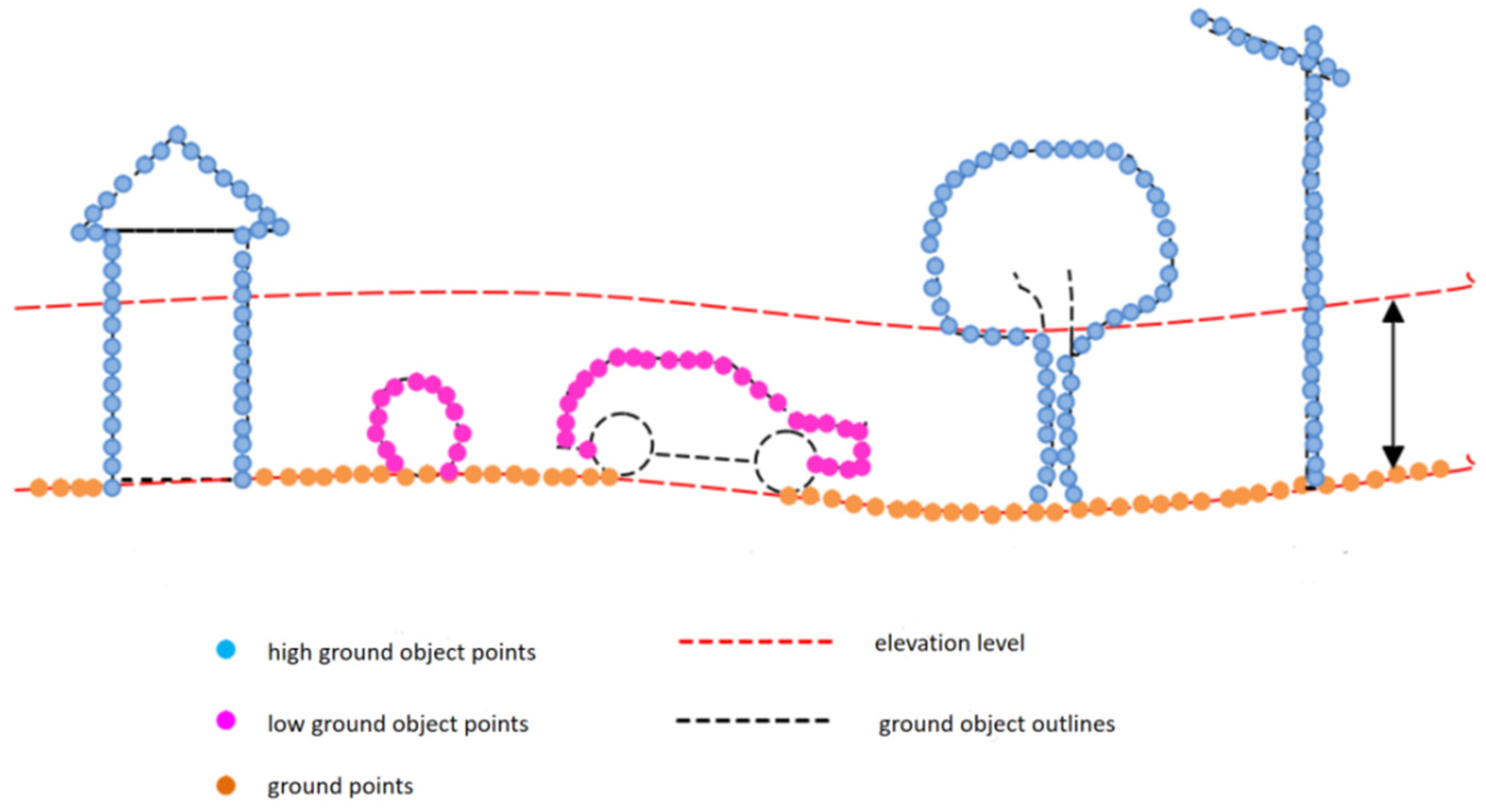
Considering to the height attribute, the common ground objects in the urban scene can be divided into three types: high ground object points, low ground object points and ground points [41], as shown in Figure 2.

The height attribute of vehicles follows market rules and can be used as a basis for removing ground points and high ground object points. The software CloudCompare [42,43] is directly used to filter ground points. Then, high ground object points of the non-ground point clouds are filtered by feature combinations [44]. The above two steps are not the core idea of the proposed method, detailed description could be found in corresponding citations. Remaining point clouds are segmented for vehicle recognition.

2.2. Neighborhood Division

As shown in Figure 1, neighborhood division in the section consists of: (1) neighborhood segmentation in the Section 2.2.1; and (2) neighborhood splitting and merging in the Section 2.2.2. The goal of the latter is to post-process the results of the former.

2.2.1. Neighborhood Segmentation

Region growth is often used for neighborhood segmentation of object recognition applications. For these applications, recent publications show that it is common to map 3D point clouds into a 2D image, which leads to the lack of 3D information of objects [45,46,47]. In the paper, neighborhood segmentation is performed based on the region growth of relative tension. We use the tension generated by the distance between point clouds to search the neighborhood by means of 3D spatial region growth.

Before describing the detailed process of neighborhood segmentation, we introduce the constraint condition of region growth in the paper.

To quantify the constraint condition between each seed point and its neighborhood points, we establish a neighboring graph for point clouds. The adjacency matrix of the graph is A, the elements of the matrix are

$$A_{ij}=\{\begin{array}{c}af{f}_{\left(ij\right)}, if p_i\in N\left(p_j\right) or p_j\in N\left(p_i\right) \\ 0, otherwise\end{array}$$

(1)

where $af{f}_{\left(ij\right)}$ is the degree of adjacency between the point $p_i$ and the point $p_j$, $N\left(p_i\right)$ represents the point set of all of the neighboring point clouds of the point $p_i$.

We use the neighboring graph to select new seed sets. A Gaussian kernel function is often used to calculate the adjacency $A_{ij}$ between the point $p_i$ and the point $p_j$ [48]:

$$af{f}_{\left(ij\right)}=exp\{\frac{-{\Vert p_i-p_j\Vert }_2}{2{\sigma }^2}\}$$

(2)

where ${\Vert p_i-p_j\Vert }_2$ represents the Euclidean distance measure.

Observing the Formula (2), we can see that the degree of adjacency is only related to the distance. The farther the distance, the lower the degree of adjacency. If the new seed point is selected based only on the Formula (2), the point closest to the original seed point will be selected. In the case of high point cloud density, this method wastes computing resource and the iteration is too slow. So, it is necessary to take a trade-off between the distance and the density. We use the linear combination of the Gaussian kernel function and the penalty term to calculate the adjacency $A_{ij}$ between the point $p_i$ and the point $p_j$. The improved adjacency is called the relative tension $r{t}_{\left(ij\right)}$ between the point $p_i$ and the point $p_j$ as follows

$$\begin{gathered} r{t}_{\left(ij\right)}=af{f}_{\left(ij\right) }+\lambda \ast {\Vert p_i-p_j\Vert }_2 \\ =exp\left\{\frac{-{\Vert p_i-p_j\Vert }_2}{2{\sigma }^2}\right\}+\lambda \ast {\Vert p_i-p_j\Vert }_2 , \lambda >0 \end{gathered}$$

(3)

where the Gaussian kernel function and the penalty term function are respectively expressed as Formulas (4) and (5), $\lambda$ > 0, the range is (0,1], it is to regulate the effects of the Gaussian kernel function and the penalty term function. And ${\Vert p_i-p_j\Vert }_2$ represents the Euclidean distance measurement. The Gaussian kernel function is related to the point density, the penalty term function is related to the distance between points. The Gaussian kernel function is defined as a monotone function of the Euclidean distance between two points in the paper.

$$f_1\left(p_i,p_j\right)=\exp \left\{\frac{-{\Vert p_i-p_j\Vert }_2}{2{\sigma }^2}\right\}$$

(4)

$$f_2\left(p_i,p_j\right)=\lambda \ast {\Vert p_i-p_j\Vert }_2$$

(5)

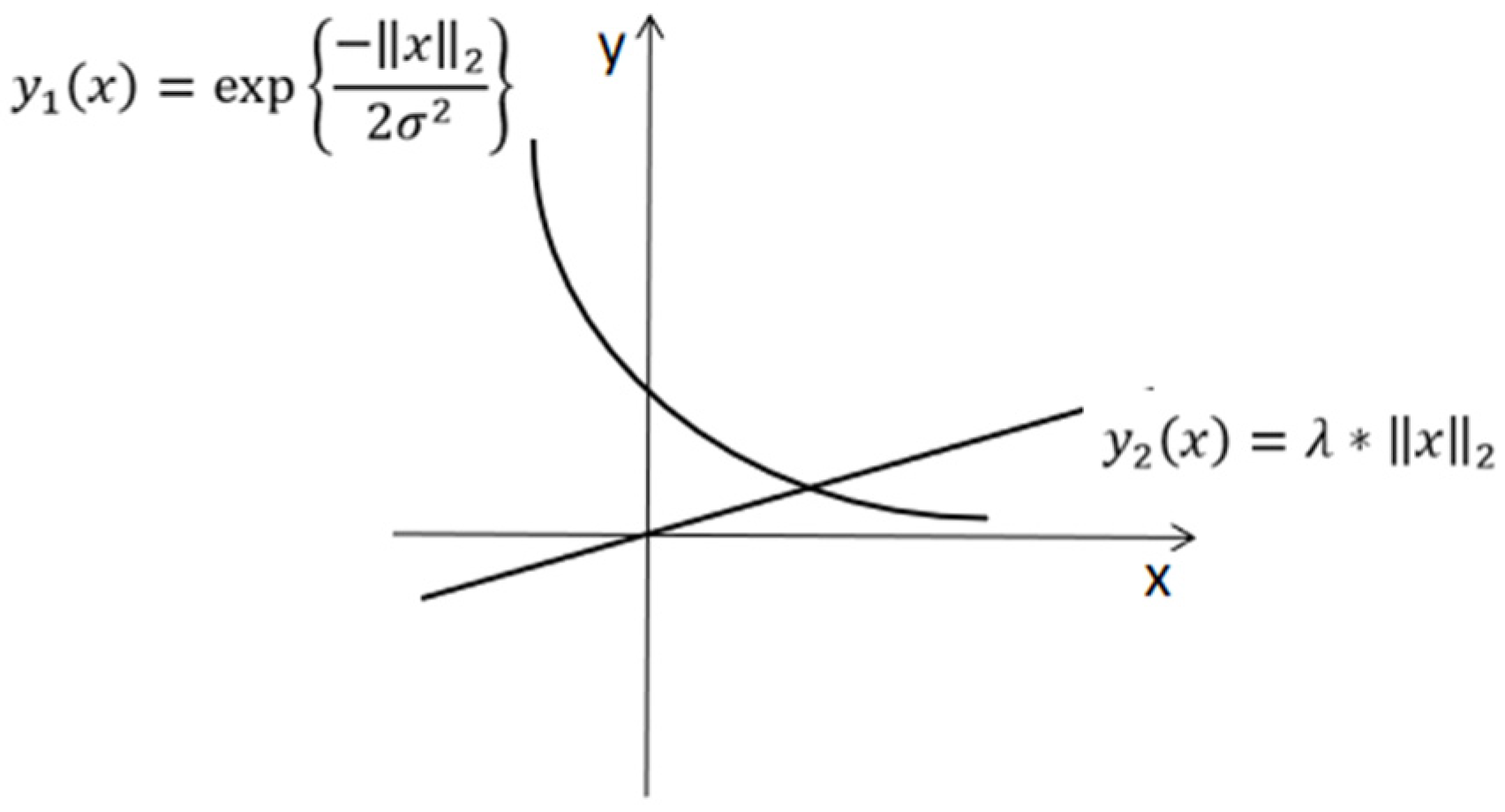
Figure 3 shows the change trend of the Gaussian kernel function and the penalty term function. It is in an inverse proportion between the Gaussian kernel function and the distance.

Based on above, the detailed process of neighborhood segmentation is as follows:

(1)

With randomly taking a seed point as the center, all points in the cube with a fixed radius are caught as its neighboring points.

(2)

According to computing the value of relative tension between the seed point and its neighboring points by Formula (3), we select several point clouds with the highest value of relative tension from these neighboring points as new seed points to form a new seed set.

(3)

We perform the same neighborhood division on the new seed set again to obtain neighboring points. These points are merged with original neighboring points into new neighboring points. New seed points are selected out again by step (2).

(4)

We iterate the above three steps. When the new seed set can no longer catch neighboring points, the algorithm stops. The area which contains the last set of neighboring points and all of the seed sets is a complete neighborhood.

A complete neighborhood may be completed by only one growth, or be completed by several growths. The incremental process ensures that the growth in each iteration step is completed on the nearest neighboring point clouds, which conforms to the first law of geography [49]. The first law of geography states that “everything is related to everything else, but near things are more related than distant things”.

Figure 4 shows the neighborhood formation process of a red seed point. The red point in Figure 4a is the initial seed point. Taking this red point as the center, point clouds in gray within a fixed radius are its neighborhood points in Figure 4a. Then we select several new seed points in Figure 4b based on the constraint conditions. Figure 4c shows the results of finding the neighboring points with the purple and brown new seed points as the center points respectively. As seen in Figure 4c, the neighboring points of the two seed points are partially overlapped. As a selected new seed point in green from neighborhood points of brown point, Figure 4d shows the results of finding the neighboring points of the green point. Figure 4e shows the neighborhood points in gray of all new seed points. Until now, the first round of searching for new seed points and their neighborhoods finishes. Then, we use the formula (3) for the seed points selected in the first round to find the new seed points and their neighborhoods in the second round. When the neighborhoods of the new seed set in the (n-1)-th round all are empty, the algorithm ends. An independent neighborhood is formed.

2.2.2. Neighborhood Splitting and Merging

As mentioned in the Section 2.2, the goal of neighborhood splitting and merging is to post-process the results of neighborhood segmentation in the Section 2.2.1, so that the segmentation results are more in line with the needs.

With region growth based on relative tension, the data set is segmented into multiple neighborhood regions. A region may contain two or more different types of objects. The goal of neighborhood splitting is to separate such different types of objects in one region further. Or one object may be divided into different regions. The goal of neighborhood merging is to combine such different regions together.

(1)

Neighborhood splitting

For the situation that a region may contain two or more different types of ground objects, we give an example to explain the neighborhood splitting method in Figure 5.

Figure 5a shows the distribution trajectory of discrete points in a 2D space. There is a gap near the interval [39,40] on the X axis. We divide the discrete points into several blocks along the X axis with a step length of 0.3, and count points in these blocks to get the histogram in Figure 5b. It is clear in Figure 5b that the number of points in the 8-th and 9-th block is zero. Therefore, we use the 8-th block as the boundary to split the original discrete points into two parts. Mathematical description of neighborhood splitting is as follows.

Recording independent regions obtained by region growth of relative tension as $R=\left\{R_1,\dots ,R_i,\dots ,R_M\right\}$, the points in the point set $R_i$ are represented by $P_i=\{p_j=\left(x_j, y_j,z_j\right)|j=1,2,\dots ,N\}$, where M is the number of regions, N is the number of point clouds in a region $R_i$. 3D coordinates of the point $p_j$ are represented by $x_j$, $y_j$ and $z_j$ respectively in a XYZ space.

To separate objects that are close but do not belong to the same category, the point clouds in a region are divided into several blocks along the parking direction of the vehicle. We count point clouds in each block and represent them by $Num=\left\{n_1,\dots ,n_i,\dots ,n_t\right\}$, where $n_i$ is the number of point clouds in $i$-th block, $t$ is the number of blocks.

If there are different types of objects in a small region, the number of point clouds in the blocks of which different objects are adjacent will be significantly small. Using this simple idea, we calculate the first derivative and the second derivative of the set $Num$. We compare the element value of the second derivative with the magnitude of zero to find the adjacent position. The calculation formulas for the first derivative and the second derivative are as follows.

The first derivative:

$$DE{R}_1=\left[de{r}_1,\dots ,de{r}_i,\dots ,de{r}_t\right]$$

(6)

$$de{r}_i=\{\begin{array}{c}0,i=1\\ n_i-n_{i-1},i\ge 2\end{array}$$

(7)

The second derivative:

$$DE{R}_2=[De{r}_1,\dots ,De{r}_i,\dots ,De{r}_t]$$

(8)

$$De{r}_i=\{\begin{array}{c}\left(1-\beta \right)\ast de{r}_i,i=1\\ \beta \ast de{r}_{i-1}+\left(1-\beta \right)\ast de{r}_i,i\ge 2\end{array}$$

(9)

where $\beta$ is the hyperparameter, generally setted to 0.5, 0.9, or 0.99.

A pseudo-code of computing the first derivative and the second derivative is given in Algorithm 1, and a pseudo-code of spitting a neighborhood into two sub-regions is given in Algorithm 2. The idea of splitting into several sub-regions is the same.

Algorithm 1: Computing the first derivative and the second derivative.

Input: $P_i=\{p_j=\left(x_j, y_j,z_j\right)|j=1,2,\dots ,N\}$,

Step length $\lambda$,

$y$ axis $\leftarrow$ parking direction,

$Y_i=\left\{y_1,\dots ,y_N\right\}$,

$V_0$ = 0, $\alpha$, $\beta$.

I:

1: t $\leftarrow$ ceil($\frac{max\left(Y_i\right)-min\left(Y_i\right)}{\lambda }$)

2: For $\mathrm{g}$: 1 to t do {

3:                 $t_1\leftarrow$ $min\left(Y_i\right)+\lambda \ast \left(g-1\right)$

4:                 $t_2\leftarrow$ $min\left(Y_i\right)+\lambda \ast g$

5:                 $t_3\leftarrow$ find($Y_i\ge t_1$ && $Y_i<t_2$)

6:                 $n\left(g\right)\leftarrow$ length($t_3$)

7:                 }

II: compute $DE{R}_1$

1: For $g$: 1 to (t $-1$) do {

2:                 $t_4\leftarrow$ $n\left(g+1\right)-n\left(g\right)$

3:                 $DE{R}_1$($g$ + $1$) $\leftarrow$ $t_4$

4:                 }

5:                 $DE{R}_1$ = [0, $DE{R}_1$]

III: compute $DE{R}_2$

1: For $g$: 1 to t do {

2:                 $t_5\leftarrow$ $\alpha \ast V_0+\beta \ast DE{R}_1\left(g\right)$

3:                 $DE{R}_2$($g$) $\leftarrow$ $t_5$

4:                 $V_0\leftarrow t_5$

5:                 }

Output:      the first derivative: $DE{R}_1$,

the second derivative: $DE{R}_2$

Algorithm 2: Spitting a neighborhood into two sub-regions.

Input: $P_i=\{p_j=\left(x_j, y_j,z_j\right)|j=1,2,\dots ,N\}$,

the first derivative: $DE{R}_1$,

the second derivative: $DE{R}_2$

1: Ind $\leftarrow$ find($DE{R}_2$ < 0)

2: l $\leftarrow$ length(Ind)

3: if l == 0

4:            P $\leftarrow$ $P_i$

5:            ind $\leftarrow$ i

6: else if l = $1$&& Ind = N

7:                        P $\leftarrow$ $P_i$

8:                        ind $\leftarrow$ i

9:else

10:            tem $\leftarrow$ Ind($1$)

11:         $P_{i1}\leftarrow \{p_j=\left(x_j, y_j,z_j\right)|j=1,2,\dots ,tem-1\}$,

12:       $P_{i2}\leftarrow \{p_j=\left(x_j, y_j,z_j\right)|j=tem-1,\dots ,N\}$,

13:            ind $\leftarrow$ [i,i].

Output: $P_i$, i or $P_{i1}$, $P_{i2}$, [i,i].

(2)

Neighborhood merging

In the section, we solve the problem of neighborhood merging. The regional fitness distance is used. Assuming that two regions to be merged, if the region $R_i$ is contained in the region $R_j$, two regions should be merged. If the region $R_i$ is separated from the region $R_j$, two regions should not be merged together. According to the value of the fitness distance in the Formula (10), we determine whether the two regions should be merged or not.

$$M\left(R_i,R_j\right)=1-\frac{size\left(b_{ij}\right)-size\left(R_i\right)-size\left(R_j\right)}{size\left(obj\right)}$$

(10)

where $b_{ij}$ is the smallest circumscribed cube of the two regions, $\mathrm{size}\left(R_i\right)$ refers to the volume of the smallest circumscribed cube of the region $R_i$, $\mathrm{size}\left(obj\right)$ refers to the volume of the smallest circumscribed cube of all regions to be merged. The higher the value, the higher the probability of merging them.

After obtaining final neighborhoods by neighborhood splitting and merging, we next catch and re-sample side projection profile of point clouds in each neighborhood in the Section 2.3.1 and Section 2.3.2. Then we measure the similarity between these side projection profiles and vehicle samples in the Section 2.3.3 and Section 2.3.4, to recognize the vehicles that fits the similarity criteria.

2.3. Similarity Measurement

To determine whether point clouds in a neighborhood belong to a vehicle or not, we can get the answer through the following four steps, also as shown in Figure 1. Here a simple logic explanation is given as follows.

(1)

In Section 2.3.1, it explains how to obtain side projection profile of point clouds in a neighborhood according to the degree of curvature of the profile curve. The side projection profile is mathematically a series of discrete points.

(2)

Generally, the point clouds of side projection profiles that obtain in (1) can not be directly involved in similarity measurement. It is necessary to re-sample the point clouds to meet the measurement conditions in the Section 2.3.2.

(3)

The unique shape of a vehicle is important information. Normal distribution measurement in Section 2.3.3 can provide the value range of vehicle length and vehicle width for removing point clouds of some of non-vehicles.

(4)

In Section 2.3.4, the principle of least squares is used to recognize point clouds of vehicles.

2.3.1. Obtaining Side Projection Profile

Due to the complex urban environment, the phenomenon of mutual occlusion among objects is widespread. When we collect data with the point cloud device moving along the road, it will cause point clouds of the obscured part of the ground objects missing. Fortunately, the vehicle data on the side near the point cloud device can be completely collected. From these data, we intentionally select out feature points to represent side projection profile of car body. Feature points are caught according to the degree of curvature of the profile curve [50].

Given a set $X=\left[X\left(1\right),\dots ,X\left(i\right),\dots ,X\left(n\right)\right]$, $n$ is the number of elements. According to the interpolation principle, the second derivative of point $X\left(i\right)$ is as follows

$$X^{″}\left(i\right)\approx \frac{1}{h^2}\left[X\left(i-h\right)-2X\left(i\right)+X\left(i+h\right)\right]$$

(11)

The curvature of a point on the curve is similar to the second derivative of that point. Suppose that the curvature of point $X\left(i\right)$ is $K$, then

$$K\approx \frac{1}{h^2}\left[X\left(i-h\right)-2X\left(i\right)+X\left(i+h\right)\right]$$

(12)

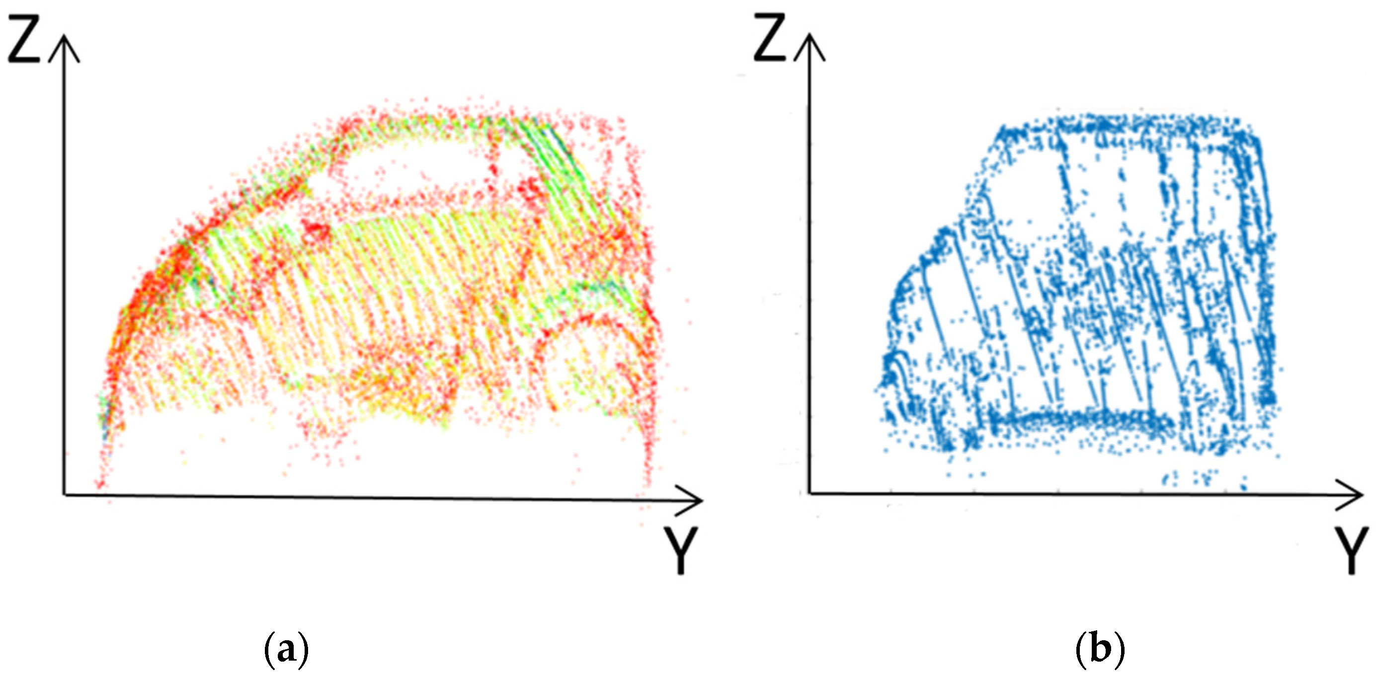
The side projection of car body is parallel to the YOZ plane from the experiment data sets, namely the Paris-Rue-Madame data set [51] and the Paris-rue-Cassette database [52]. We project point clouds in each neighborhood to the YOZ plane. Two discrete point sets based on the Y and Z directions can be obtained. According to formula (12), feature points are extracted in the Y and Z directions respectively. Point clouds at the index positions of the feature points in the two directions are combined to describe original side projection profile of car body. Figure 6 shows the profile projection and feature points of the point cloud data of a vehicle on the YOZ plane. It gives the projection profile of the vehicle on the YOZ plane based on original collected points in Figure 6a. Figure 6b shows the selected feature points of the vehicle according to the degree of curvature of the profile curve. Compared with Figure 6a, the number of points in Figure 6b has decreased significantly. These feature points are caught to accurately and concisely delineate the contour of the vehicle.

2.3.2. Re-Sampling Side Projection Profile

The side projection profile of car body is mathematically a series of discrete points. The number of discrete points for different types of vehicles is not the same. To better measure the similarity of the side projection profile of car body, it is necessary to keep the numbers of discrete points equal [53]. This work is carried out by re-sampling the original side profile based on the side profile of the sample vehicle.

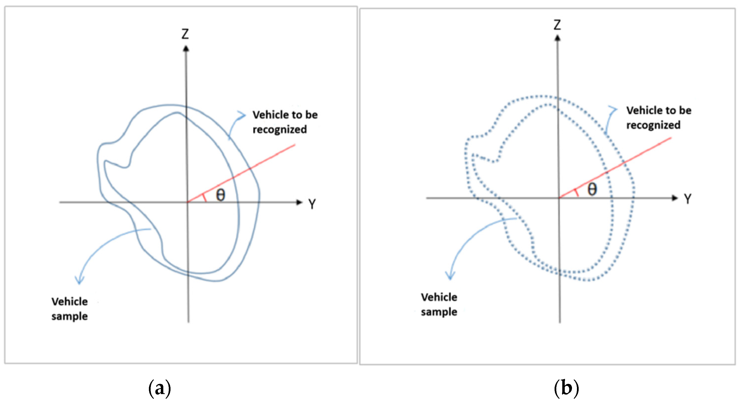
The re-sampling process is as follows. First, we establish a 2D YOZ coordinate system. The horizontal and vertical axes of the coordinate system are consistent with Y and Z values of vehicle point clouds. The origin of the coordinate system is the center of gravity of the projection profile of sample car body. Starting from the positive Y axis in the counterclockwise direction with theta angle as the interval, we draw a ray with an inclination angle from the origin of the coordinate system to intersect the side profile of the sample vehicle and the point clouds to be recognized on the YOZ plane. Intersection points are the resampled profile points, denoted as $\left(y_{a,k},z_{a,k}\right)$, $\left(y_{b,k},z_{b,k}\right)$, where $k=1,2,\dots ,n;n=\raisebox{1ex}{$360$}\!\left/ \!\raisebox{-1ex}{$\theta $}\right.$. If there is no intersection, a point closest to the ray is selected. Figure 7a shows the complete side projection profiles of the point clouds to be recognized and the vehicle sample on the YOZ plane. Figure 7b shows the side projection profiles after re-sampling. To ensure a sufficient density of sampling points, the angle sampling interval in the paper is 1°.

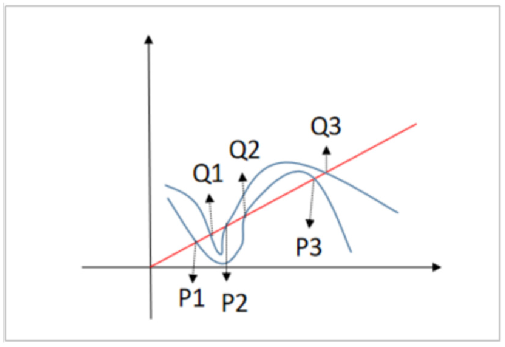
For the type of non-convex side profile, there may be more than one intersection point between the ray at a certain angle and the side profile, as shown in Figure 8. We deal with the problem as follows.

According to the ray direction, the intersection points between the ray and the side profile of the sample vehicle are recorded as

$$P_a=\left\{P_{a,1},\dots ,P_{a,i},\dots ,P_{a,m1}\right\}=\left\{\left(y_{a,1},z_{a,1}\right),\left(y_{a,2},z_{a,2}\right),\dots ,\left(y_{a,m1},z_{a,m1}\right)\right\}$$

(13)

Specifically, $m1$ is the number of the intersection points between the ray and the side projection profile of the sample vehicle.

The intersection points between the ray and the side projection profile of the point clouds to be recognized are recorded as

$$P_b=\left\{P_{b,1},\dots ,P_{b,i},\dots ,P_{b,m2}\right\}=\left\{\left(y_{b,1},z_{b,1}\right),\left(y_{b,2},z_{b,2}\right),\dots ,\left(y_{b,m2},z_{b,m2}\right)\right\}$$

(14)

Specifically, $m2$ is the number of intersection points between the ray and the side projection profile of the point clouds to be recognized.

If $m1$ and $m2$ are equal, then $P_{a,i}$ and $P_{b,i}$ are marked as the corresponding point pair. For example, (P1, Q1), (P2, Q2), (P3, Q3) in Figure 8 are the corresponding point pairs. If these two numbers of intersection points are not equal, the intersection points between the angle ray and the two side profiles are discarded.

It gives an example of re-sampling the side projection profile of point clouds of a vehicle in Figure 9. According to the degree of curvature of the profile curve, Figure 9a shows the side projection profile of feature points of the vehicle. Figure 9b shows the side projection profile of the vehicle after re-sampling. By comparison, the side projection profile of the vehicle is still well preserved to meet normal distribution measurement in Section 2.3.3 and similarity measurement of side projection profile in Section 2.3.4.

After re-sampling the side projection profile, a set S of corresponding point pairs is obtained:

$$\begin{gathered} S=\{\left(\left(y_{a,1},z_{a,1}\right),\left(y_{b,1},z_{b,1}\right),\left(y_{c,1},z_{c,1}\right),\dots ,\left(y_{g,1},z_{g,1}\right)\right), \\ ⋮ \\ \left(\left(y_{a,i},z_{a,i}\right),\left(y_{b,i},z_{b,i}\right),\left(y_{c,i},z_{c,i}\right),\dots , \left(y_{g,i},z_{g,i}\right)\right), \\ ⋮ \\ \left(\left(y_{a,k},z_{a,k}\right),\left(y_{b,k},z_{b,k}\right),\left(y_{c,k},z_{c,k}\right),\dots , \left(y_{g,k},z_{g,k}\right)\right), \\ i=1,\dots ,k; k=1,2,\dots ,n;n=\raisebox{1ex}{$360$}\!\left/ \!\raisebox{-1ex}{$\theta $}\right.\} \end{gathered}$$

(15)

where $g$ is the number of intersection point pairs between the sample vehicle and point clouds to be recognized.

2.3.3. Normal Distribution Measurement

The unique shape of a vehicle is important information to recognize it from complex urban environment. We consider two factors of body length and body width in the paper, which are defined as follows [54]:

Body length: the longest distance of the car point clouds in the length direction.

Body width: the farthest distance of the car point clouds in the width direction. The width of the vehicle body does not include the extended width of the left and right rearview mirrors (that is, the folded width of the rearview mirrors).

Taking into account the experiment data sets in the paper, the shape sizes of cars refer to European standards.

Table 1. Size information of the best-selling cars in the European market.

Number	Brand	Model	Body Length (mm)	Body Width (mm)
1	Volkswagen	Golf	4262	1799
2	Tesla	Model 3	4694	1850
3	Ford	Focus	4647	1810
4	Renault S.A.	Clio	4063	1732
5	Benz	Class A	4622	1796
6	Skoda	Octavia	4675	1814
7	Nissan	Qashqai	4401	1837
8	Toyota	Yaris	4160	1700
9	Ford	Fiesta	3980	1722
10	Mini	Hatch	3832	1727
11	Opel	Corsa	3741	1608
12	Citroen	C3	3850	1667
13	Renault S.A.	Captur	4122	1778
14	BMW	Series 1	4341	1765
15	Volvo	XC60	4688	1902
16	Peugeot	208	3962	1739
17	Toyota	Corolla	4635	1780
18	Volkswagen	Polo	4053	1740
19	Volkswagen	Tiguan	4486	1839
20	F.I.A.T.	500X	3547	1627
21	Smart	Smart	2695	1663
22	Renault S.A.	Magotan	4865	1832
23	Benz	Class E	5065	1860
24	Benz	Class S	5259	1899
25	Peugeot	5008	4670	1855
26	BMW	X5	4930	2004
27	Audi	Q3	4518	1843
28	Porsche	911	4519	1852
29	Hyundai	Encino	4195	1800
30	Suzuki	SX4	4135	1755

shows the size information of the best-selling cars in the European market.

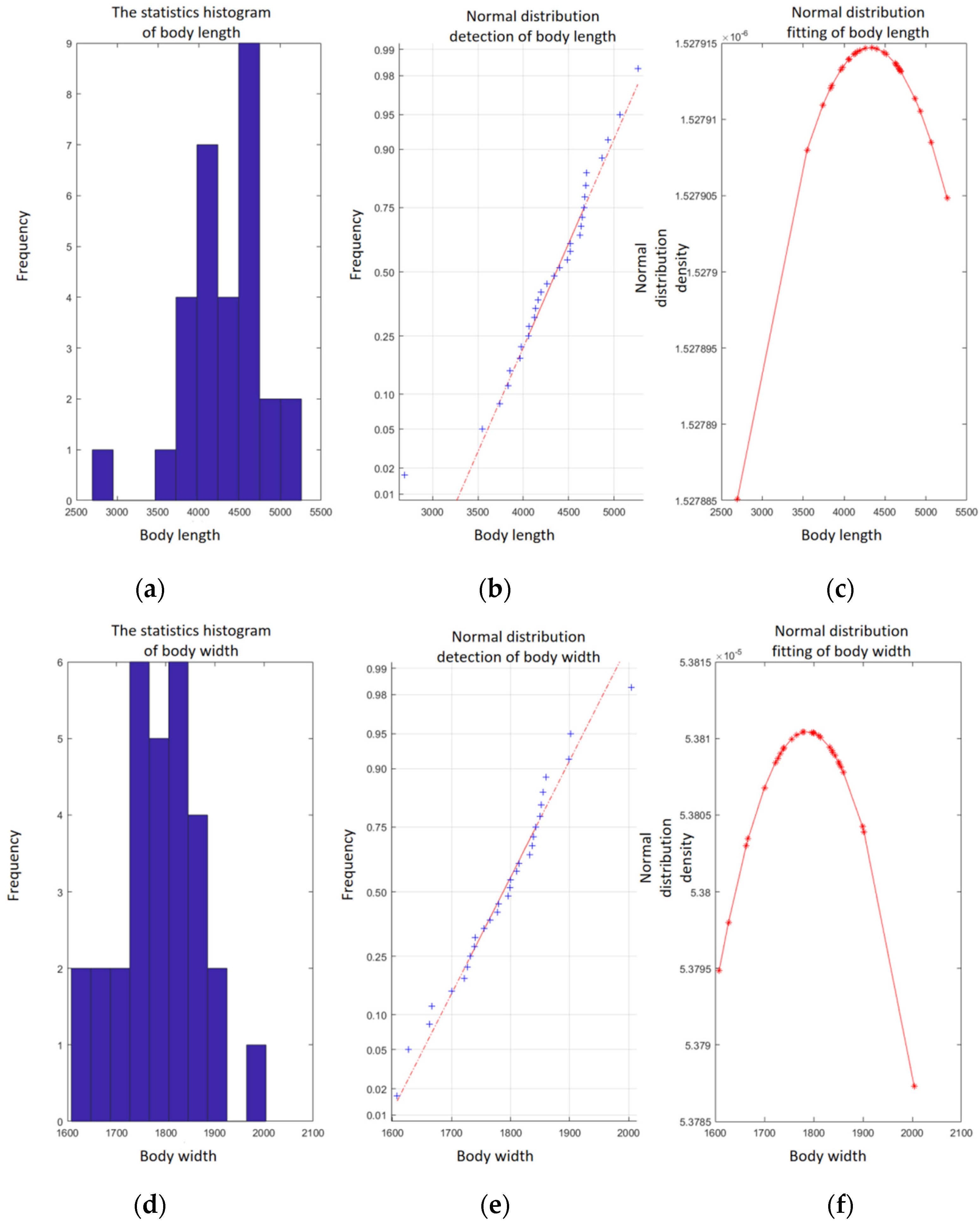
After counting the body length and body width of 30 best-selling cars in the European market, corresponding histogram and normal distribution fitting are shown in Figure 10.

The vehicle length/width statistical histogram shows the relationship between length/width and the corresponding frequency. The vehicle length/width normal distribution detection is to test whether the vehicle length/width conforms to the normal distribution or not. If the “+” point basically coincides with the red straight line, it can be considered as satisfying the normal distribution. The vehicle length/width normal distribution fitting gives the relationship between the vehicle length/width and the normal distribution density. The value corresponding to the horizontal axis at the apex of the red curve is the average value of vehicle length/width. Based on normal distribution law, the value range of vehicle length and vehicle width are computed for removing point clouds of some of non-vehicles.

2.3.4. Similarity Measurement of Side Projection Profile

In above sections, we obtain corresponding point sets of both the sample vehicle and side projection profile of point clouds to be recognized after re-sampling in the Formula (15). We select out corresponding point sets which meet normal distribution measurement to measure their similarity of side projection profiles.

Due to the unique structure of the vehicle shape, there is no rotation deformation among the side projection profiles of vehicle body for the same type of vehicles. There is only translation and zoom deformation. Coordinate transformation model used for similarity measurement can be expressed as

$$\{\begin{array}{c}{y}_g={\lambda }_{ay}\ast y_a+{\lambda }_{by}\ast y_b+\dots +{\lambda }_{fy}\ast y_f+dy\\ z_g={\lambda }_{az}\ast z_a+{\lambda }_{bz}\ast z_b+\dots +{\lambda }_{fz}\ast z_f+dz\end{array}$$

(16)

The corresponding points in the point set S are brought into the Formula (16). The principle of least squares is used to find the parameters $\left({\lambda }_y,{\lambda }_z,dy,dz\right)$, that is, to solve the linear formula as $Ay=b$. The expression of $A,y,b$ are as follows:

$$A=\left(\begin{array}{c}\begin{array}{ccc}{y}_{a,1}& y_{b,1}& \cdots \\ 0& 0& \cdots \\ ⋮& ⋮& \cdots \end{array} \begin{array}{ccc}{y}_{f,1}& 0& 0\\ 0& z_{a,1}& z_{b,1}\\ ⋮& ⋮& ⋮\end{array} \begin{array}{ccc}\cdots & 0& 1\\ \cdots & z_{f,1}& 0\\ \cdots & ⋮& ⋮\end{array} \begin{array}{c}0\\ 1\\ ⋮\end{array}\\ \begin{array}{ccc}{y}_{a,k}& y_{b,k}& \cdots \\ 0& 0& \cdots \end{array} \begin{array}{ccc}{y}_{f,k}& 0& 0\\ 0& z_{a,k}& z_{b,k}\end{array} \begin{array}{ccc}0& 0& 1\\ \cdots & z_{f,k}& 0\end{array} \begin{array}{c}0\\ 1\end{array}\end{array}\right)$$

(17)

$$y={\left({\lambda }_{ay},\dots ,{\lambda }_{fy},{\lambda }_{az},\dots ,{\lambda }_{fz},dy,dz\right)}^T$$

(18)

$$b={\left(y_{g,1},z_{g,1},\dots ,y_{g,k},z_{g,k}\right)}^T$$

(19)

After obtaining parameters of the similarity measurement model, we convert the side profile of point clouds to be measured as $\left(\overline{y_{a,j}},\overline{z_{a,j}}\right)$, and the calculation formula is

$$\{\begin{array}{c}\overline{y_{a,j}}=y_{a,j}\ast {\lambda }_y+dy\\ \overline{z_{a,j}}=z_{a,j}\ast {\lambda }_z+dz\end{array}$$

(20)

The overall similarity error between point clouds to be measured and side profile data points of the sample vehicle is $v={\displaystyle \sum }_{j=1}^g\raisebox{1ex}{$v_j^2$}\!\left/ \!\raisebox{-1ex}{$n$}\right.$, the similarity residual of a single point is represented as $v_j=\sqrt{{\left(y_{a,j}-\overline{y_{a,j}}\right)}^2+{\left(z_{a,j}-\overline{z_{a,j}}\right)}^2}$.

To achieve the optimal similarity measurement, it is necessary to iteratively perform the above computing process until the overall similarity error no longer changes.

3. Results and Discussion

In the section, vehicle recognition results are given. Selection of two parameters radius and seed number, and performance of each step in the Section 2.2 are discussed.

3.1. Vehicle Recognition Results

In this section, experiments are tested on the open source data set [51]. The data set consists of two files, which are referred by the area A and area B. Figure 11 shows the street view in the area A and area B.

To quantitatively assess the accuracy of vehicle recognition results, we adopt the following three indices: recall, precision, and F-score [55]. In the paper, recall evaluates the ratio of the correctly recognized objects to the ground truth; precision measures the ratio of the correctly recognized objects to all of the recognized components; F-score is an overall measure. The three indices are defined as follows: recall = TP/(TP + FN), precision = TP/(TP + FP), and F-score = 2*recall*precision/(recall + precision), where TP, FN, and FP denote the numbers of true positives, false negatives, and false positives, respectively.

Table 2. The results of recognizing vehicle points on Pari-Rue-Madame database.

Data Set	Recall	Precision	F-Score
Paris-Rue-Madame database	0.837	0.979	0.902

gives the results of vehicle recognition on the Paris-rue-Madame database [51] under three indices. The proposed algorithm achieves a recall, precision, and F-score of 0.837, 0.979 and 0.902, respectively.

Table 3. The results of recognizing actual vehicles on Pari-Rue-Madame database.

Data Set			Right	Left	Erroneous
Paris-Rue-Madame database	In the area A (Left in Figure 11)	Ground truth	8	19	-
		Recognition result	7	16	4
	In the area B (Right in Figure 11)		Right	Left	Erroneous
		Ground truth	13	11	-
		Recognition result	12	10	2

gives the results of the number of cars that exist versus the number of cars that are successfully separated on the Paris-rue-Madame database [51]. According to the proposed method, 45 vehicles are extracted from actual 51 cars, and the accuracy is 0.882.

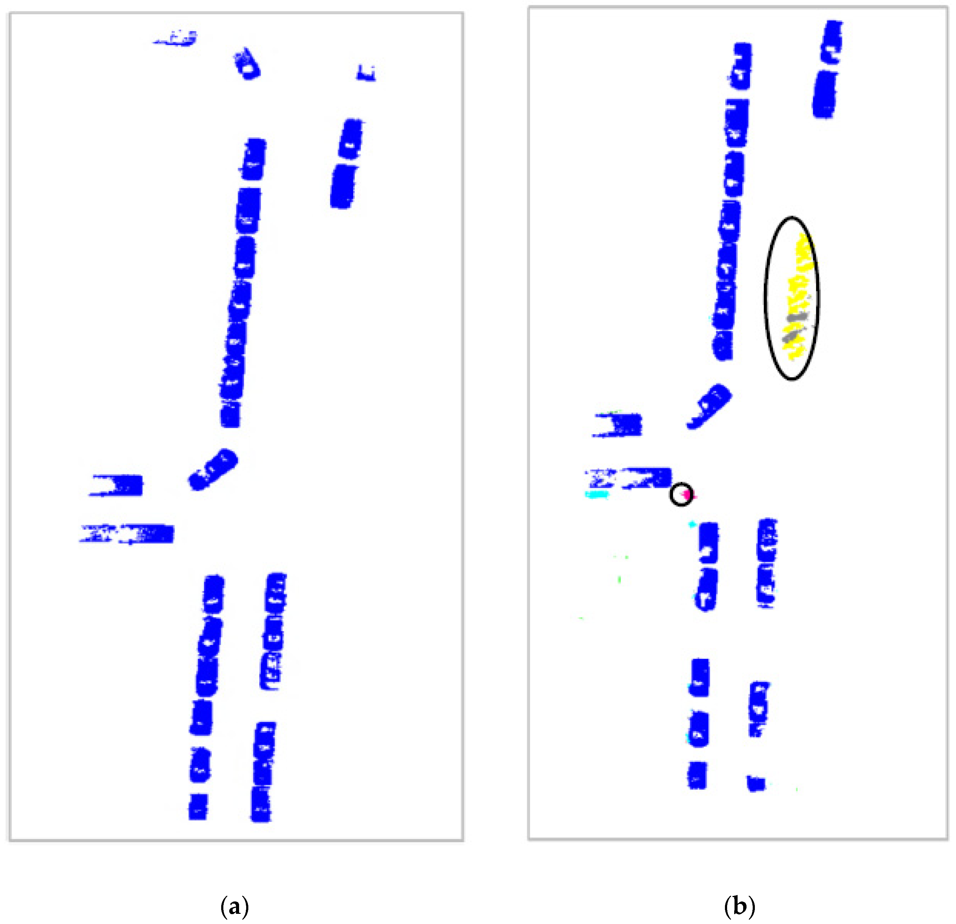
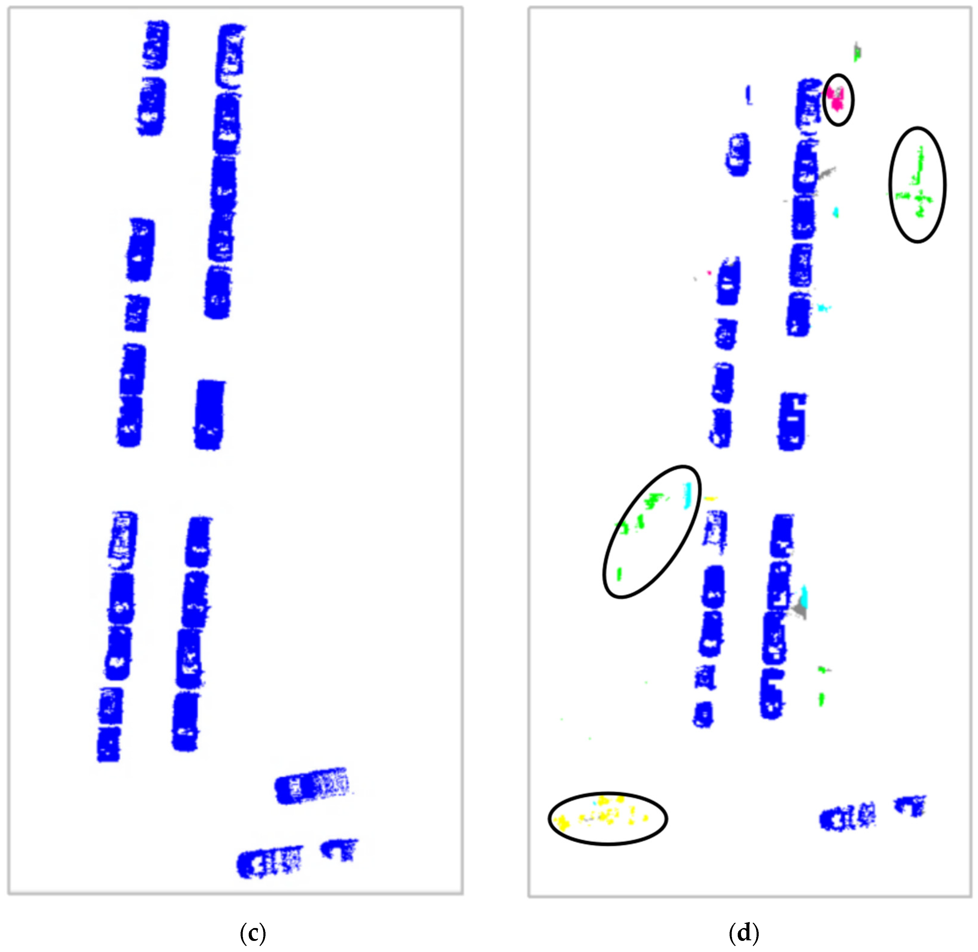
Figure 12 visualizes the view comparison of vehicle recognition results with ground truth in regions A and B. It shows actual location of vehicles in the area A in Figure 12a. Figure 12b shows the recognized vehicles and their locations in the area A. By comparison, most of the vehicles are successfully recognized, and the vehicles in the middle of the road also can be successfully recognized. Several motorcycles in yellow and other objects are mistakenly recognized as vehicles. The height attribute of vehicles is used as a basis for removing ground points and high ground object points in Section 2.1. It is similar in height attribute for vehicles and motorcycles. Motorcycle point clouds, as part of remaining point clouds, are misidentified as vehicles. Figure 12c shows actual location of vehicles in the area B, and Figure 12d shows the recognized vehicles and their locations in the area B. By comparison, most of the vehicles are successfully recognized, and the vehicles at the end of the road can also be successfully recognized. Several motorcycles in yellow, attachments of building in green and other objects in other colors are mistakenly recognized as vehicles. More features need to be explored to avoid such errors.

Additionally, the proposed algorithm runs on a computer with Intel(R) Core(TM) I7-7700HQ CPU @ 2.80 GHz with 4 cores, RAM 16.0 GB. The programming language is in MATLAB. The detailed computing time in each processing step is listed in

Table 4. Computing time (minute).

Data Set	Point Cloud Pre-Removing	Neighborhood Division	Similarity Measurement	Total
Paris-Rue-Madame data set	15	38	2	55

. The total time cost for recognizing vehicles on the Paris-Rue-Madame data set is about 55 min. Specifically, the processing time for point cloud pre-removing is about 15 min, the processing time for neighborhood division is about 38 min, the processing time for similarity measurement is about 2 min.

3.2. Selection of Parameters Radius and Seed Number

The influence of parameters the radius and the seed number per segmentation in Section 2.2.1 on vehicle recognition performance and computation time is explored in the section.

Figure 13 shows the value change trend of three indices (recall, precision, and F-score) and computation time with the variation of parameter radius. As the radius increases, the computation time decreases, precision value almost keeps stable, both the recall value and the F-score value increase first and then decrease. Comprehensively, the result should be optimal when R equals to 0.5.

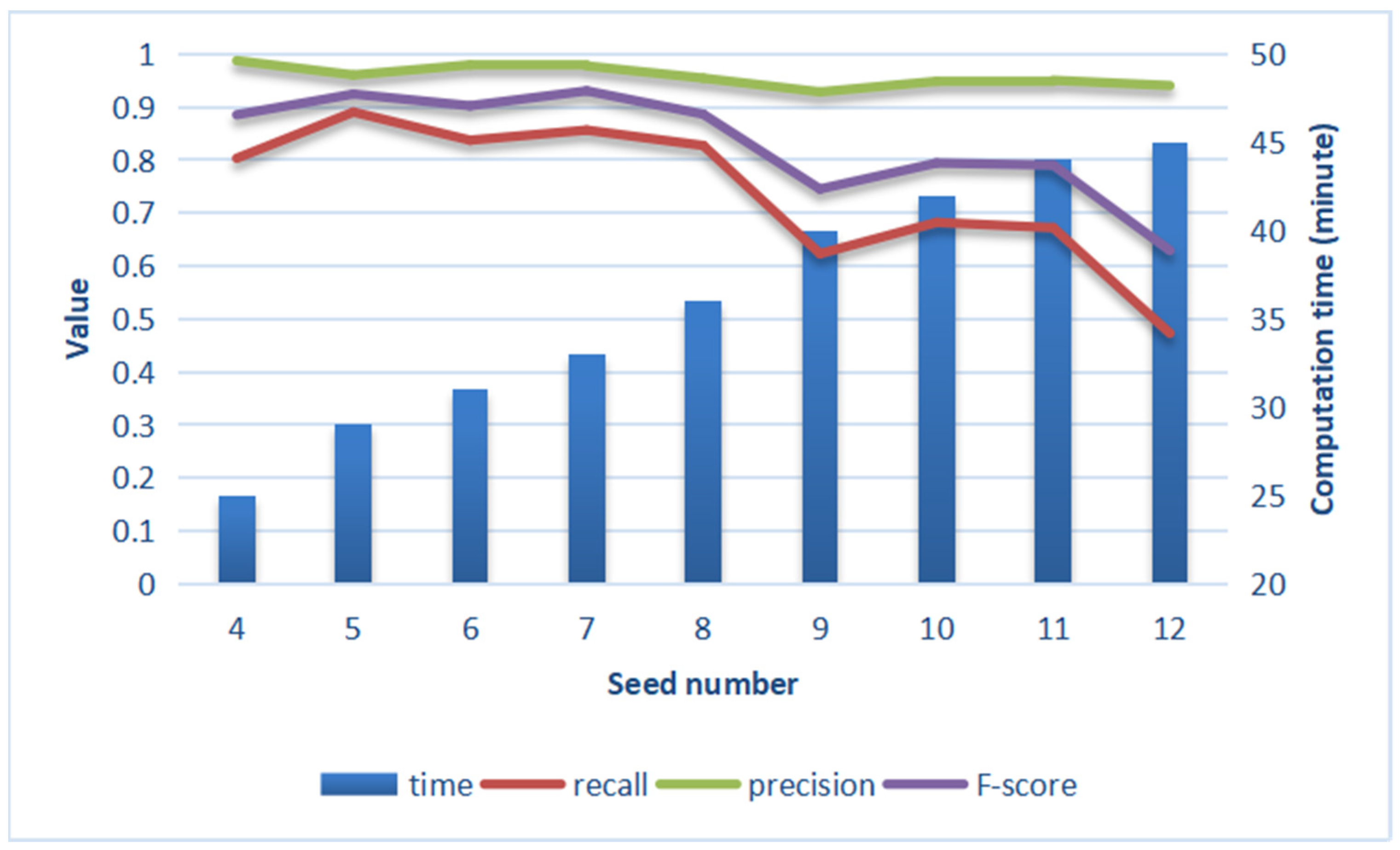
Figure 14 shows the value change trend of three indices (recall, precision, and F-score) and computation time with the variation of parameter seed number. As the seed number increases, the computation time increases, precision value almost keeps stable, both the recall value and the F-score value keep stable first and then decrease. Comprehensively, the result should be optimal when seed number equals to 5.

From Figure 13 and Figure 14, the computation time is inversely proportional to the radius value, but proportional to the seed number. For the convenience, the reason behind computation time difference with the variation of parameters radius and seed number is explained in a two-dimensional space. Figure 15 shows the results of finding the neighboring points with the red\green\blue seed points as the center points respectively. When every seed point looks for its neighborhood points, the point clouds in the gray region is retrieved once. Compared Figure 15a,b, the smaller the radius value, the more point clouds are repeatedly retrieved, and the longer the computation time. Compared Figure 15c,d, the more the seed number, the more point clouds are repeatedly retrieved, and the longer the computation time.

3.3. Performance of Region Growth Based on Relative Tension

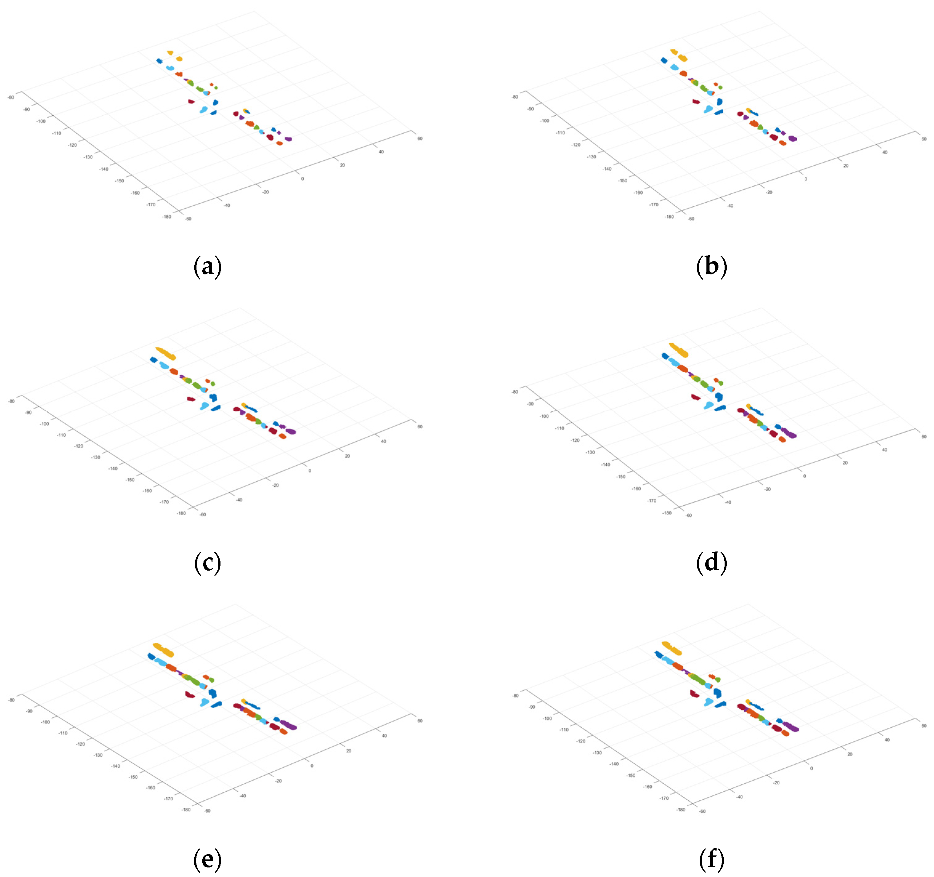
Figure 16 shows neighborhood changes of region growth based on relative tension during the incremental iterative process. Different neighborhoods are displayed in different colors. From Figure 16a–f, the shapes of colorful blocks gradually become larger. From shape and position distribution of the neighborhoods in Figure 16f, 3D neighborhoods obtained by the proposed method conforms to the law of vehicle distribution. Point cloud distribution obviously conforms to the parking rules of vehicles on both sides of the road. Different colorful blocks are arranged in two parallel straight lines (on both sides of the road). A few blocks appear in the vertical direction in the center of the road, which represent cars turning at the intersection.

Furthermore, to get a clearer picture of local results in Figure 16, without loss of generality, partial neighborhood segmentation results are shown in Figure 17. In Figure 17, for example, one vehicle in each black ellipse is divided into multiple small areas. The examples exactly demonstrate the necessity of neighborhood splitting and merging.

3.4. Performance of Neighborhood Splitting and Merging

As introduced in the Section 2.2.2 and the example in Figure 17, the data set is segmented into multiple neighborhood regions. A region may contain two or more different types of objects. Or one object may be divided into different regions. The purpose of neighborhood splitting and merging is to make one object as completely divided into an independent region as possible. Without loss of generality, we give two examples to illustrate the usefulness of the proposed method.

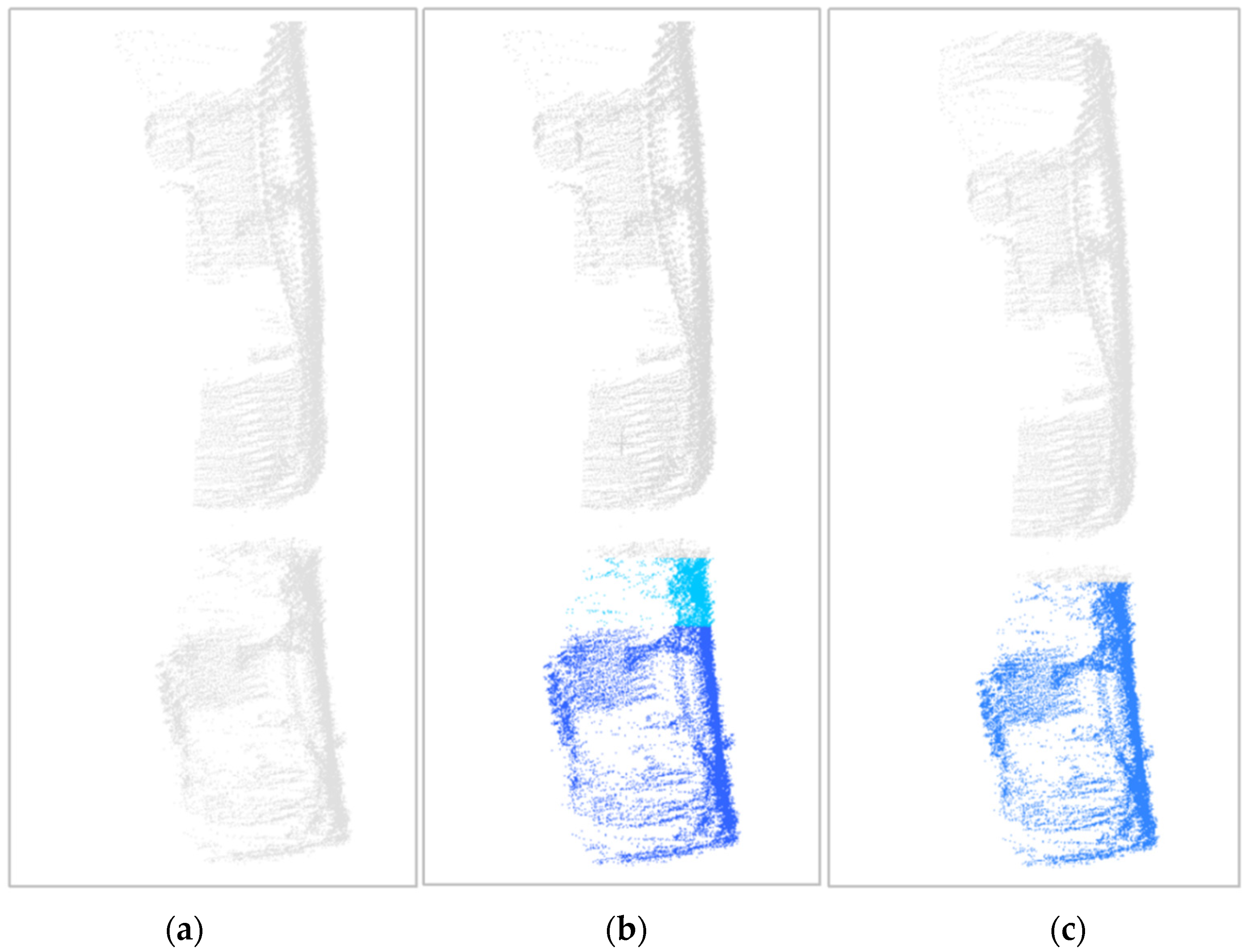
Figure 18 shows an example of neighborhood splitting and merging. By region growth based relative tension, Figure 18a shows two cars are segmented into one region in gray. We divide them into several small regions according to the proposed neighborhood splitting method. The smaller car is divided into two regions in dark blue and light blue, as shown in Figure 18b. Figure 18c gives the result of neighborhood merging. Two small regions belonging to the same car in Figure 18b are successfully merged together.

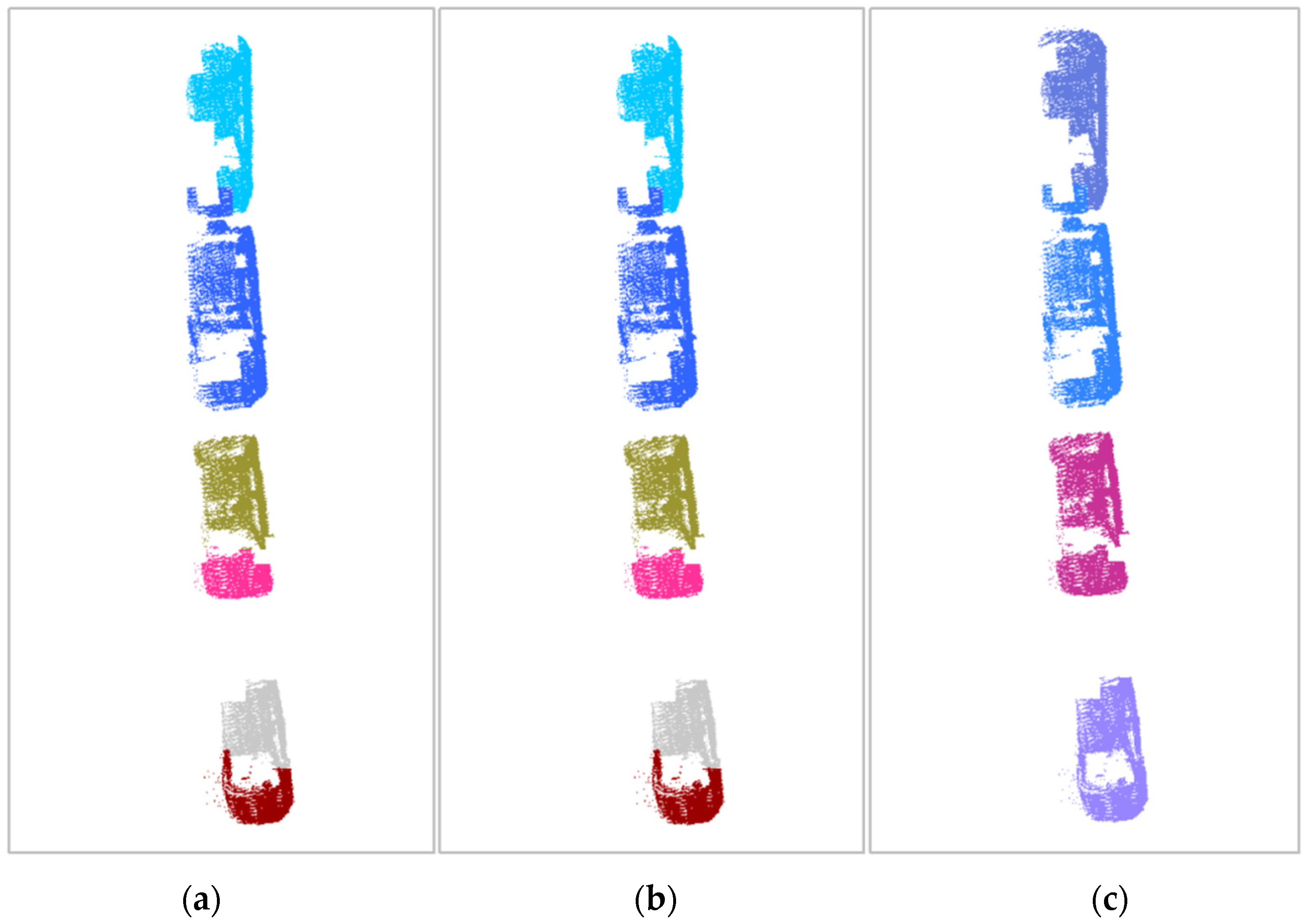
Figure 19 shows another example of neighborhood splitting and merging effect. It is the neighborhood segmentation result by region growth based relative tension in Figure 19a. The four vehicles are divided into six regions by neighborhood segmentation and indicated by six colors. On the basis of the results, Figure 19b shows the neighborhood splitting result. On the basis of the result in Figure 19b, it is the neighborhood merging result in Figure 19c. In Figure 19a, each vehicle is represented by either one color or multiple colors. There is no obvious case that multiple vehicles are in the same color. According to the Algorithms 1 and 2 in the Section 2.2.2, vehicles do not be split again. So Figure 19a,b are completely the same. In Figure 19c, the areas in yellow-green and rose red in Figure 19b have been successfully merged into vehicles in dark purple. The areas in gray and wine red have been merged successfully into a vehicle in lavender.

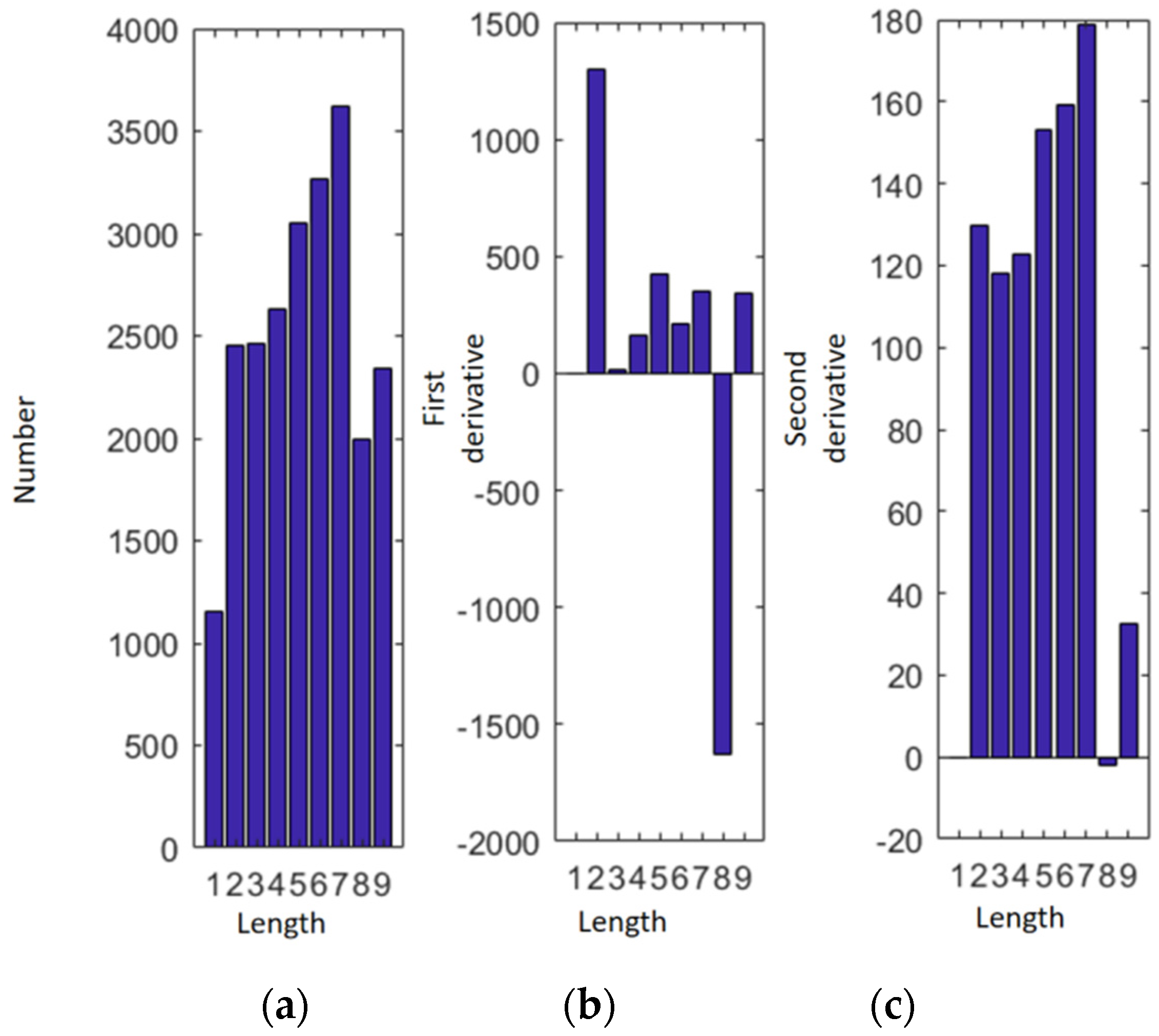
Let’s take the smaller car in Figure 18 to analyze the mathematical principles behind neighborhood splitting and merging. Figure 20 shows number change of point clouds in the area where the smaller car is located, and its first and second derivatives. The value of the second derivative is less than 0 at the length “8” in Figure 20c.

According to Algorithm 2, we split the point clouds in the area into two small regions at the length “8”, namely the regions in dark blue and in light blue in Figure 18b. We calculate the fitness distance of these two small areas according to the Formula (10)

$$M=1-\frac{6.7949-5.2851-0.9636}{6.7949}=0.9196$$

By computation, $M$ is greater than 0.9. These two small regions need to be merged.

4. Comparative Studies

The comparison between the proposed method and existing work are presented from four aspects in the section.

4.1. Recognition Result Indices

A performance comparison on car recognition is conducted on the publicly available Paris-Rue-Madame data set [51], between the proposed method and the existing methods [20,56,57]. Brief description of these three existing methods are given below.

A new methodology for large-scale urban 3D point cloud classification is described [20]. The main contribution is an in-depth analysis of a powerful strategy for recovering individual 3D neighborhoods of optimal size. The most crucial issue of the whole methodology remains an appropriate selection of the scale parameter, which generally requires a higher computational effort due to the consideration of individual 3D neighborhoods of optimal size.

An effective and efficient method for point-wise semantic classification is proposed to handle unstructured and inhomogeneous point clouds [56]. The contribution of the present paper is a feature set that addresses both variations in point density and computational efficiency, which turns out to be careful handling of neighborhood relations.

A new, fully automatic and versatile framework is presented [57]. 5 different neighborhood definitions, 21 features, 6 approaches for feature subset selection and 2 different classifiers are evaluated to explore optimal neighborhoods for individual 3D point classification. In addition to the large time consumption, the non-obvious feature-class correlation affects the accuracy of vehicle recognition.

The comparison results for the Paris-rue-Madame database [51] are listed in

Table 5. Comparison results between the proposed and three existing methods on [51].

Data Set	Method	Recall	Precision	F-Score
Paris-Rue-Madame data set	Hackel et al. [56]	0.9786	0.9086	0.9423
	Weinmann et al. [20]	0.6476	0.7948	0.7137
	Weinmann et al. [57]	0.603	0.768	0.676
	Proposed	0.837	0.979	0.902

. The best results are respectively in bold. The proposed algorithm achieves a recall, precision, and F-score of 0.837, 0.979 and 0.902, respectively. By comparison, the proposed method keep competitive performances on recall, precision, and F-score value. Although a lower recall value, the proposed approach obtains the best precision to recognize cars, and the F-score result is excellent and near the best result value. This strength comes from the use of physical characteristics of vehicles that provides distinct information, which improves their recognition.

The proposed method also is tested on the Paris-rue-Cassette database [52]. The comparison results between the proposed method and two previous work are given in

Table 6. Comparison results between the proposed and two existing methods on [52].

Data Set	Method	Recall	Precision	F-Score
Paris-Rue-Cassette data set	Hackel et al. [56]	0.9307	0.8608	0.8943
	Weinmann et al. [20]	0.6112	0.6767	0.6423
	Proposed	0.9496	0.7832	0.8584

. The best results are respectively in bold. The proposed algorithm achieves a recall, precision, and F-score of 0.9496, 0.7832 and 0.8584, respectively. The proposed approach obtains the best Recall, and the F-score result is excellent and near the best result value.

4.2. Neighborhood Segmentation Performance

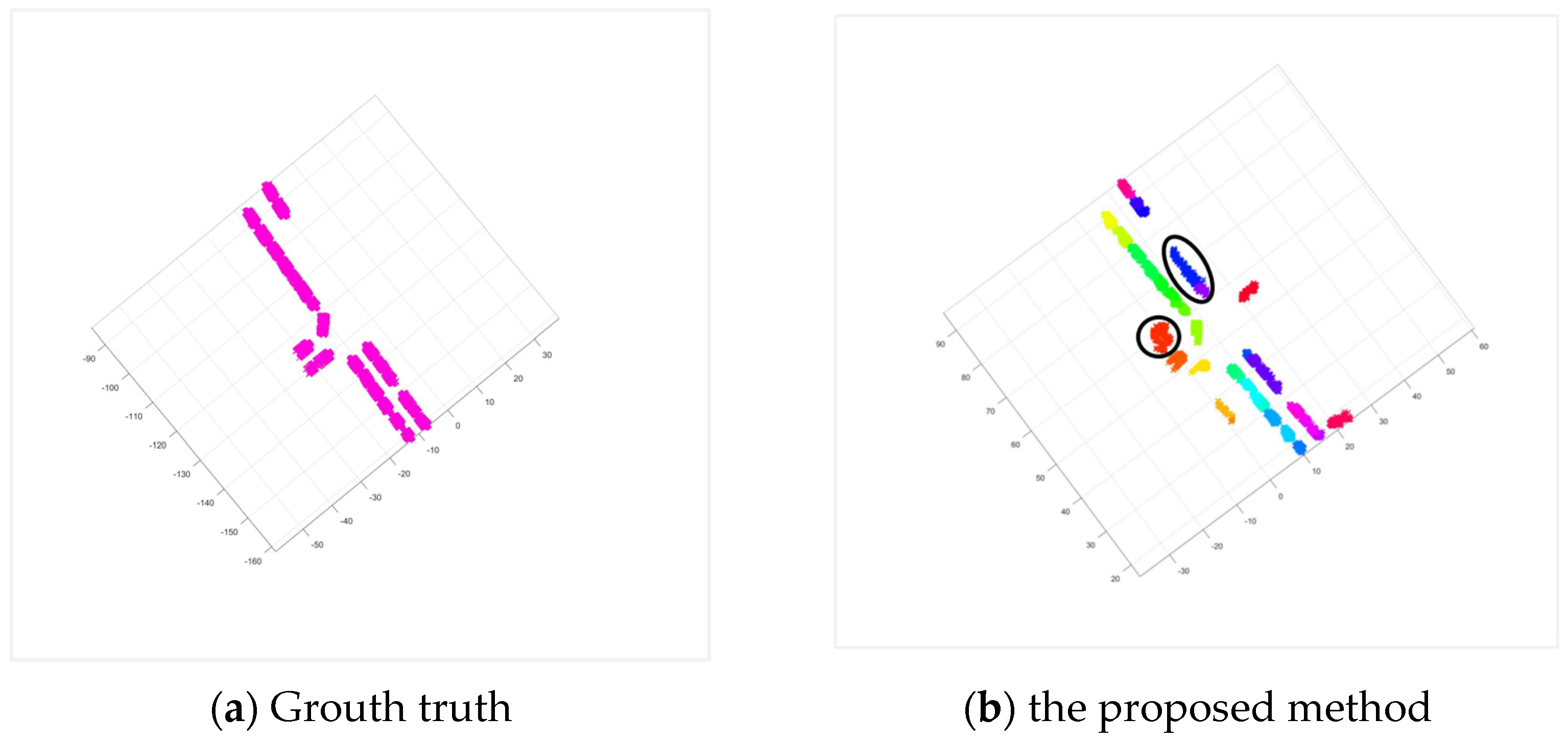
Figure 21 provides side-by-side comparisons of neighborhood segmentation among highly relevant algorithms DBCSAN [58], kmeans [59], mean shift [60], and the proposed method for the Paris-rue-Madame database [51]. Figure 21a,c,e,g show the ground truth. Vehicles are distinguished by different colors. In Figure 21b,d,f,h, neighborhood segmentation results by four algorithms are displayed. Different neighborhoods are displayed in different colors.

As expected, the general tread is that most neighborhoods of vehicles in Figure 21b,d,f,h are correctly segmented and overall appearance is matched with ground truth quite well. Specifically, comparing color chromatic aberration in these four figures, the proposed method best preserves the independence among vehicles. However, there are cases where slight differences occur. Errors are highlighted in the black ellipses in Figure 21b,d,f,h. In Figure 21b, vehicle neighborhoods are correctly segmented, but point clouds of some of non-vehicles in the black ellipses are mistakely kept by the proposed method. In Figure 21d, the independence among vehicles is not obvious, and the segmentation results by the DBSCAN include a few non-vehicle point clouds. In Figure 21f, beside mistakes in the black ellipses, the problem with the neighborhood segmentation by the kmeans is the fragmentation. Most vehicles consist of neighborhood fragmentations in several colors. These fragmentations can reduce similarity measurement performance. In Figure 21h, point clouds of some of non-vehicles are kept and point clouds of some of vehicles are missed, as shown in the black ellipses, which will negatively affect the accuracy of vehicle recognition. More feature combinations in the Section 2.1 could be further explored to help reduce such errors in removing point clouds of non-vehicles.

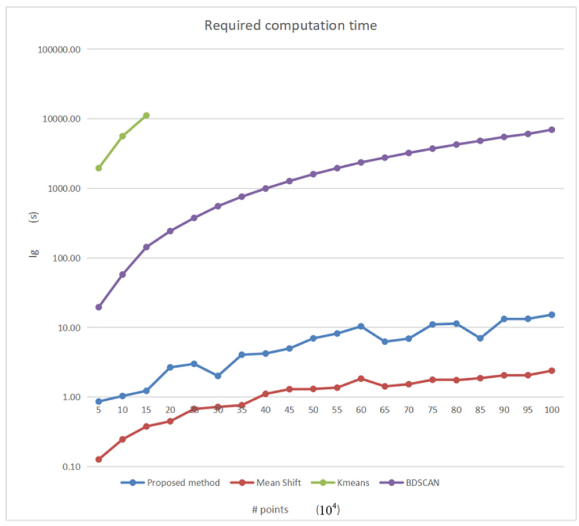
Additionally, compared with the proposed method and mean shift algorithm, kmeans and DBSCAN algorithms are more prone to computation time problem when the number of point clouds is too large. The comparison of computation time is given in next section.

4.3. Computation Time

Concerning the computational complexity, we may consider the computation time required for processing different numbers of point clouds. In Figure 22, this is carried out for neighborhood segmentation of DBCSAN, kmeans, mean shift and the proposed method. To show the computational complexity more clearly, the vertical axis shows the logarithmic value of computation time. It becomes apparent that both the proposed method and mean shift algorithm show superior computational advantage for increasing numbers of considered 3D points. The computational burden of BDSCAN algorithm is significantly heavier than the proposed method and mean shift algorithm. Three given values in green line in Figure 22 reflect that required computation time is the most difficult problem when considering kmeans algorithm.

4.4. Recognition Performance for Specific Situations

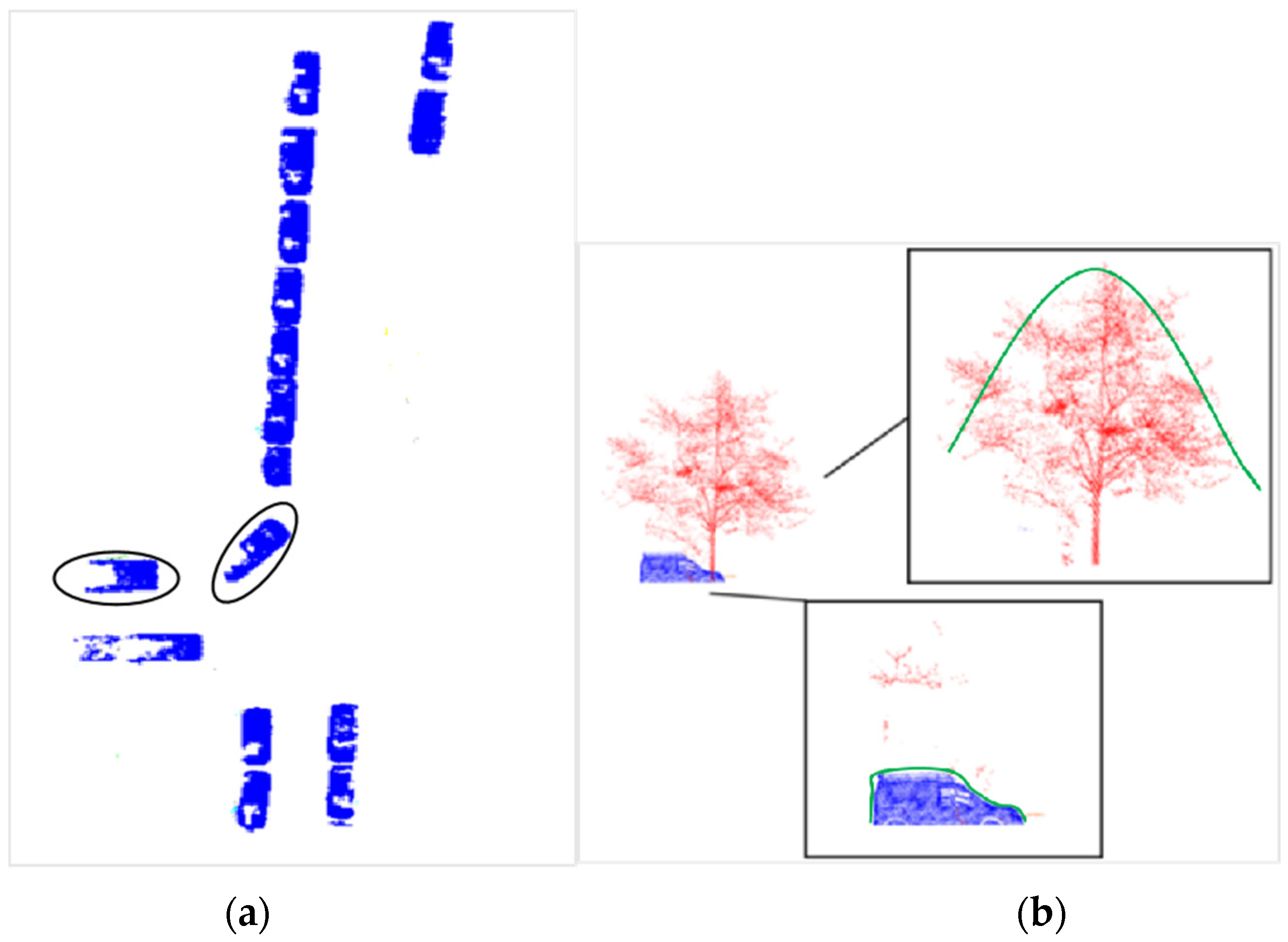
The existing methods are limited to complex situations such as objects overlap. Some moving cars which were distorted also failed to be recognized by them. Comparatively, benefited from side projection profile properties of vehicle body, the proposed method is able to deal with those cars that overlapped with the trees. The core of the neighborhood division algorithm in this paper is the spatial tension between point clouds. Figure 23 shows the vehicle recognition advantage of the proposed method in these limitation situations of above three methods for the Paris-rue-Madame database [51]. Figure 23a shows that the moving vehicles in the black ellipses are well recognized by the proposed method. Figure 23b presents that the proposed algorithm can separate well the vehicles and trees that overlap in the Z direction. The separation between trees and vehicles comes from two aspects. On the one hand, the operation of point cloud pre-removing in the Section 2.1 could filter some of tree points in the Z direction. On the other hand, there are great difference in the size and side projection profile between vehicles and trees, as shown in green curve in Figure 23b. These differences play a key role in recognizing the vehicles. Spaces between trees and vehicles in the Z direction also help separate each other.

5. Conclusions

We propose to recognize urban vehicles based on region growth of relative tension and similarity measurement of side projection profile of vehicle body in the paper. Quantitative evaluations on the selected data set show that the proposed algorithm achieves a recall, precision, and F-score of 0.837, 0.979 and 0.902 respectively. Experiments show that region growth algorithm based on relative tension well guarantees the integrity and independence of physical structures of vehicles. Although part of 3D data of vehicle point clouds are missing, side projection profile of car body in 2D plane is complete. It enables similarity measurement method of the side projection profile to successfully recognize neighborhoods that contain point clouds of vehicles. Comparative studies demonstrate the superior advantage of the proposed algorithm in vehicle recognition result, neighborhood segmentation performance and computation time. In conclusion, by using point cloud data, we have provided a promising and effective solution to accurate recognition of road scene vehicles toward transportation related applications. Further exploration on both touching cars and a car driven template would foster even stronger the proposed method in the future work.

References

1. Yu, Y.; Zheng, H. Vehicle detection from high resolution satellite imagery based on the morphological neural network. J. Harbin Eng. Univ. 2006, 7, 189–193. [Google Scholar]
2. Moon, H.; Chellappa, R.; Rosenfeld, A. Performance analysis of a simple vehicle detection algorithm. Image Vis. Comput. 2002, 20, 1–13. [Google Scholar] [CrossRef]
3. Zhao, T.; Nevatia, R. Car detection in low resolution aerial image. In Proceedings of the 8th IEEE International Conference on Computer Vision, Washington, DC, USA, 7–14 July 2001. [Google Scholar]
4. Ruskone, R.; Guiges, L.; Airault, S.; Jamet, O. Vehicle detection on aerial images: A structural approach. In Proceedings of the 13th International Conference on Pattern Recognition, Vienna, Austria, 25–29 August 1996. [Google Scholar]
5. Cheng, G.; Han, J.; Zhou, P.; Xu, D. Learning rotation-invariant and fisher discriminative convolutional neural networks for object detection. IEEE Trans. Image Process. 2019, 28, 265–278. [Google Scholar] [CrossRef]
6. Yang, C.; Li, W.; Lin, Z. Vehicle Object Detection in Remote Sensing Imagery Based on Multi-Perspective Convolutional Neural Network. Int. J. Geo-Inf. 2018, 7, 249. [Google Scholar] [CrossRef] [Green Version]
7. Wu, X.; Hong, D.; Tian, J.; Chanussot, J.; Li, W.; Tao, R. ORSIm detector: A novel object detection framework in optical remote sensing imagery using spatial-frequency channel features. IEEE Trans. Geosci. Remote Sens. 2019, 57, 5146–5158. [Google Scholar] [CrossRef] [Green Version]
8. Kang, L.; Gellert, M. Fast multiclass vehicle detection on aerial images. IEEE Geosci. Remote Sens. Lett. 2015, 12, 1938–1942. [Google Scholar] [CrossRef] [Green Version]
9. Cheng, G.; Si, Y.; Hong, H.; Yao, X.; Guo, L. Cross-scale feature fusion for object detection in optical remote sensing images. IEEE Geosci. Remote Sens. Lett. 2020, 18, 431–435. [Google Scholar] [CrossRef]
10. Wu, X.; Hong, D.; Chanussot, J.; Xu, Y.; Tao, R.; Wang, Y. Fourier-based rotation-invariant feature boosting: An efficient framework for geospatial object detection. IEEE Geosci. Remote Sens. Lett. 2020, 17, 302–306. [Google Scholar] [CrossRef] [Green Version]
11. Yang, B.; Liang, F.; Huang, R. Progress, Challenges and Perspectives of 3D LiDAR Point Cloud Processing. Acta Geod. Cartogr. Sin. 2017, 46, 1509–1516. [Google Scholar]
12. Park, J.; Kim, C.; Jo, K. PCSCNet: Fast 3D Semantic Segmentation of LiDAR Point Cloud for Autonomous Car using Point Convolution and Sparse Convolution Network. arXiv 2022, arXiv:2202.10047. [Google Scholar] [CrossRef]
13. Zou, T.; Chen, G.; Li, Z.; He, W.; Qu, S.; Gu, S.; Knoll, A. KAM-Net: Keypoint-Aware and Keypoint-Matching Network for Vehicle Detection from 2D Point Cloud. IEEE Trans. Artif. Intell. 2022, 3, 207–217. [Google Scholar] [CrossRef]
14. Yang, B.; Dong, Z.; Zhao, G.; Dai, W. Hierarchical extraction of urban objects from mobile laser scanning data. ISPRS J. Photogramm. Remote Sens. 2015, 99, 45–57. [Google Scholar] [CrossRef]
15. Zhang, Y.; Ge, P.; Xu, J.; Zhang, T.; Zhao, Q. Lidar-based Vehicle Target Recognition. In Proceedings of the 4th CAA International Conference on Vehicular Control and Intelligence, Hangzhou, China, 18–20 December 2020. [Google Scholar]
16. Li, B. 3d fully convolutional network for vehicle detection in point cloud. In Proceedings of the IEEE International Conference on Intelligent Robots and Systems, Vancouver, BC, Canada, 24–28 September 2017. [Google Scholar]
17. Wang, H.; Zhang, X. Real-time vehicle detection and tracking using 3D LiDAR. Asian J. Control. 2022, 24, 1459–1469. [Google Scholar] [CrossRef]
18. Liang, X.; Fu, Z. MHNet: Multiscale Hierarchical Network for 3D Point Cloud Semantic Segmentation. IEEE Access. 2019, 7, 173999–174012. [Google Scholar] [CrossRef]
19. Weinmann, M.; Jutzi, B.; Mallet, C. Feature relevance assessment for the semantic interpretation of 3D point cloud data. ISPRS Ann. Photogramm. Remote Sens. Spat. Inf. Sci. 2013, 5, 313–318. [Google Scholar] [CrossRef] [Green Version]
20. Weinmann, M.; Urban, S.; Hinz, S.; Jutzi, B.; Mallet, C. Distinctive 2D and 3D features for automated large-scale scene analysis in urban areas. Comput. Graph. 2015, 49, 47–57. [Google Scholar] [CrossRef]
21. Weinmann, M.; Weinmann, M.; Mallet, C.; Brédif, M. A classification-segmentation framework for the detection of individual trees in dense MMS point cloud data acquired in urban areas. Remote Sens. 2017, 9, 277. [Google Scholar] [CrossRef] [Green Version]
22. Wu, Z.; Song, S.; Khosla, A.; Yu, F.; Zhang, L. 3d shapenets: A deep representation for volumetric shapes. In Proceedings of the IEEE conference on Computer Vision and Pattern Recognition, Boston, MA, USA, 7–12 June 2015; pp. 1912–1920. [Google Scholar]
23. Maturana, D.; Scherer, S. Voxnet: A 3d convolutional neural network for real-time object recognition. In Proceedings of the International Conference on Intelligent Robots and Systems, Hamburg, Germany, 28 September–2 October 2015; pp. 922–928. [Google Scholar]
24. Gorte, B. Segmentation of TIN-structured surface models. Int. Arch. Photogramm. Remote Sens. Spat. Inf. Sci. 2002, 34, 465–469. [Google Scholar]
25. Yu, L. Research on Methods for Ground Objective Classification and Rapid Model Construction Based on Mobile Laser Scanning Data. Ph.D. Thesis, Wuhan University, Wuhan, China, 2011. [Google Scholar]
26. Mohamed, M.; Morsy, S.; El-Shazly, A. Evaluation of data subsampling and neighbourhood selection for mobile LiDAR data classification. Egypt. J. Remote Sens. Space Sci. 2021, 24, 799–804. [Google Scholar] [CrossRef]
27. Mohamed, M.; Morsy, S.; El-Shazly, A. Evaluation of machine learning classifiers for 3D mobile LiDAR point cloud classification using different neighborhood search methods. Adv. LiDAR 2022, 2, 1–9. [Google Scholar]
28. Seyfeli, S.; OK, A.O. Classification of Mobile Laser Scanning Data with Geometric Features and Cylindrical Neighborhood. Baltic J. Mod. Comput. 2022, 10, 209–223. [Google Scholar] [CrossRef]
29. Xu, J.; Zhang, R.; Dou, J.; Zhu, Y.; Sun, J.; Pu, S. Rpvnet: A deep and efficient range-point-voxel fusion network for lidar point cloud segmentation. In Proceedings of the IEEE International Conference on Computer Vision, Montreal, QC, Canada, 11–17 October 2021; pp. 16024–16033. [Google Scholar]
30. Xu, Y.; Tong, X.; Stilla, U. Voxel-based representation of 3D point clouds: Methods, applications, and its potential use in the construction industry. Autom. Constr. 2021, 126, 103675. [Google Scholar] [CrossRef]
31. Dai, J.; Qi, H.; Xiong, Y.; Li, Y. Deformable convolutional networks. In Proceedings of the IEEE International Conference on Computer Vision, Venice, Italy, 22–29 October 2017; pp. 764–773. [Google Scholar]
32. Mohamed, M.; Morsy, S.; El-Shazly, A. Improvement of 3D LiDAR point cloud classification of urban road environment based on random forest classifier. Geocarto Int. 2022, 37, 15604–15626. [Google Scholar] [CrossRef]
33. Geng, H.; Gao, Z.; Fang, G.; Xie, Y. 3D Object Recognition and Localization with a Dense LiDAR Scanner. Actuators 2022, 11, 13. [Google Scholar] [CrossRef]
34. Zhang, T.; Vosselman, G.; Elberink, S.J.O. Vehicle recognition in aerial LiDAR point cloud based on dynamic time warping. ISPRS Ann. Photogramm. Remote Sens. Spatial Inf. Sci. 2017, IV-2/W4, 193–198. [Google Scholar] [CrossRef] [Green Version]
35. Zhang, T.; Kan, Y.; Jia, H.; Deng, C.; Xing, T. Urban vehicle extraction from aerial laser scanning point cloud data. Int. J. Remote Sens. 2020, 41, 6664–6697. [Google Scholar] [CrossRef]
36. Shi, S.; Jiang, L.; Deng, J.; Wang, Z.; Guo, C.; Shi, J.; Wang, X.; Li, H. PV-RCNN++: Point-voxel feature set abstraction with local vector representation for 3D object detection. arXiv 2021, arXiv:2102.00463. [Google Scholar] [CrossRef]
37. Li, J.; Dai, H.; Shao, L.; Ding, Y. From voxel to point: Iou-guided 3d object detection for point cloud with voxel-to-point decoder. In Proceedings of the 29th ACM International Conference on Multimedia, Virtual Event, China, 20–24 October 2021; pp. 4622–4631. [Google Scholar]
38. Zhou, W.; Cao, X.; Zhang, X.; Hao, X.; Wang, D.; He, Y. Multi Point-Voxel Convolution (MPVConv) for Deep Learning on Point Clouds. arXiv 2021, arXiv:2107.13152. [Google Scholar]
39. Roynard, X.; Deschaud, J.; Goulette, F. Classification of point cloud scenes with multiscale voxel deep network. arXiv 2018, arXiv:1804.03583. [Google Scholar]
40. Su, H.; Maji, S.; Kalogerakis, E. Multi-view convolutional neural networks for 3d shape recognition. In Proceedings of the IEEE International Conference on Computer Vision, Santiago, Chile, 13–16 December 2015; pp. 945–953. [Google Scholar]
41. Zhang, X. Studying on the information extraction of streetlight and street tree from vehicle-borne LiDAR point cloud. Master’s Thesis, Henan Polytechnic University, Jiaozuo, China, 2017. [Google Scholar]
42. Zhang, W.; Qi, J.; Wan, P.; Wang, H.; Xie, D.; Wang, X.; Yan, G. An Easy-to-Use Airborne LiDAR Data Filtering Method Based on Cloth Simulation. Remote Sens. 2016, 8, 501. [Google Scholar] [CrossRef]
43. Girardeau-Montaut, D. Cloud Compare; Électricité de France, S.A., Ed.; (EDF) R&D: Paris, France, 2003. [Google Scholar]
44. Zheng, M.; Wu, H.; Li, Y. An adaptive end-to-end classification approach for mobile laser scanning point clouds based on knowledge in urban scenes. Remote Sens. 2019, 11, 186. [Google Scholar] [CrossRef] [Green Version]
45. Kang, C.; Wang, F.; Zong, M.; Cheng, Y.; Lu, T. Research on improved region growing point cloud algorithm. Int. Arch. Photogramm. Remote Sens. Spat. Inf. Sci. 2020, 42, 153–157. [Google Scholar] [CrossRef] [Green Version]
46. Alshawabkeh, Y. Linear feature extraction from point cloud using color information. Herit. Sci. 2020, 8, 1–13. [Google Scholar] [CrossRef]
47. Xie, Y.; Tian, J.; Zhu, X. Linking points with labels in 3D: A review of point cloud semantic segmentation. IEEE Geosci. Remote Sens. Mag. 2020, 8, 38–59. [Google Scholar] [CrossRef] [Green Version]
48. Huang, R.; Sang, N.; Liu, L.Y.; Luo, D.P.; Tang, J.L. A Method of Clustering Feature Vectors via Incremental Iteration. PR&AI 2010, 23, 320–326. [Google Scholar]
49. Tobler, W.R. A Computer Movie Simulating Urban Growth in the Detroit Region. Econ. Geogr. 1970, 46, 234. [Google Scholar] [CrossRef]
50. Liu, Y.; Ge, Q. An indirect algorithm for contour feature extraction. Compu Eng. Appl. 2004, 10, 51–52+70. [Google Scholar]
51. Serna, A.; Marcotegui, B.; Goulette, F.; Deschaud, J.E. Paris-rue-Madame database: A 3D mobile laser scanner dataset for benchmarking urban detection, segmentation and classification methods. In Proceedings of the 4th International Conference on Pattern Recognition Applications and Methods (ICPRAM 2014), Angers, France, 6–8 March 2014. [Google Scholar]
52. Vallet, B.; Brédif, M.; Serna, A.; Marcotegui, B.; Paparoditis, N. TerraMobilita/iQmulus Urban Point Cloud Analysis Benchmark. Comput. Graph. 2015, 49, 126–133. [Google Scholar] [CrossRef] [Green Version]
53. Li, L.; Han, Y. Building contour matching in airborne LiDAR point clouds. Remote Sens. Inf. 2016, 2, 13–18. [Google Scholar]
54. Wang, H. Vehicle identification and classification system based on laser ranging. Master’s Thesis, Tianjin University, Tianjin, China, 2011. [Google Scholar]
55. Yu, Y.; Li, J.; Guan, H.; Wang, C.; Yu, J. Semiautomated extraction of street light poles from mobile LiDAR point-clouds. IEEE Trans. Geosci. Remote Sens. 2015, 53, 1374–1386. [Google Scholar] [CrossRef]
56. Hackel, T.; Wegner, J.D.; Schindler, K. Fast Semantic Segmentation of 3d Point Clouds with Strongly Varying Density. ISPRS Ann. Photogramm. Remote Sens. Spat. Inf. Sci. 2016, 3, 177–184. [Google Scholar]
57. Weinmann, M.; Jutzi, B.; Mallet, C. Semantic 3D scene interpretation: A framework combining optimal neighborhood size selection with relevant features. ISPRS Int. Arch. Photogramm. Remote Sens. Spat. Inf. Sci. 2014, II-3, 181–188. [Google Scholar] [CrossRef] [Green Version]
58. Schubert, E.; Sander, J.; Ester, M.; Kriegel, H.P.; Xu, X. DBSCAN revisited, revisited: Why and how you should (still) use DBSCAN. ACM Trans. Database Syst. 2017, 42, 1–21. [Google Scholar] [CrossRef]
59. Hartigan, J.A.; Wong, M.A. A K-Means Clustering Algorithm. Appl. Stat. 1979, 28, 100. [Google Scholar] [CrossRef]
60. Comaniciu, D.; Meer, P. Mean shift analysis and applications. In Proceedings of the 7th IEEE International Conference on Computer Vision, Kerkyra, Greece, 20–27 September 1999. [Google Scholar]
Figure 1. The workflow of vehicle recognition based on region growth of relative tension and similarity measurement of side projection profile of vehicle body.
Remotesensing 15 01493 g001
Figure 2. Ground object points based on height attribute.
Remotesensing 15 01493 g002
Figure 3. The change trend of the Gaussian kernel function and the penalty term function.
Remotesensing 15 01493 g003
Figure 4. Neighborhood formation process of a red seed point. (ae): non-gray dots: seed points; purple box: the neighboring region with the purple seed point as the center point; the same goes for other colorful boxes.
Remotesensing 15 01493 g004
Figure 5. Neighboring splitting analysis of discrete points on a 2D plane. Note: display of 2D discrete points (a); the statistics of the number of point clouds in blocks (b).
Remotesensing 15 01493 g005
Figure 6. Side projection profile of a vehicle on YOZ plane. Note: based on original collected points (a); based on selected feature points of the vehicle (b). (Red, green: different reflectance values of point clouds).
Remotesensing 15 01493 g006
Figure 7. Re-sampling the side projection profile of the point clouds to be recognized. Note: before re-sampling (a); after re-sampling (b).
Remotesensing 15 01493 g007
Figure 8. Selection of the corresponding point pairs.
Remotesensing 15 01493 g008
Figure 9. An example of re-sampling the side projection profile of point clouds of a vehicle. Note: before re-sampling (a); after re-sampling (b).
Remotesensing 15 01493 g009
Figure 10. Normal distribution fitting of body size of the best-selling cars in the European Market. Note: The statistics histogram of body length/width of the best-selling cars (a,d); normal distribution detection of body length/width of the best-selling cars (b,e); normal distribution fitting of body length/width of the best-selling cars (c,f).
Remotesensing 15 01493 g010
Figure 11. The street view in the area A (a) and area B (b). Note: Vehicles in dark blue, other objects in different colors (buildings in green, motorcycles in yellow, ground in gray, trash cans in red, others in light blue).
Remotesensing 15 01493 g011
Figure 12. The view comparison of vehicle recognition results with ground truth in regions A and B. Note: actual location of vehicles respectively in the area A and B (a,c); vehicle recognition results respectively in the area A and B (b,d). Vehicles in dark blue (ad), objects in other colors are misidentified as vehicles (b,d).
Remotesensing 15 01493 g012aRemotesensing 15 01493 g012b
Figure 13. The value change trend of three indices (recall, precision, and F-score) and computation time with the variation of the parameter radius.
Remotesensing 15 01493 g013
Figure 14. The value change trend of three indices (recall, precision, and F-score) and computation time with the variation of the parameter seed number.
Remotesensing 15 01493 g014
Figure 15. The reason behind computation time difference with the variation of parameters radius and seed number ((a,b): different radii; (c,d): different seed numbers). (Gray: the region within all points; red circle: the neighboring region with the red seed point as the center point; the same goes for other colorful circles).
Remotesensing 15 01493 g015
Figure 16. Neighborhood changes of region growth based on relative tension during the iterative process. Different neighborhoods are displayed in different colors. (af): different neighborhood segmentation results during the incremental iterative process.
Remotesensing 15 01493 g016
Figure 17. Partial neighborhood results of region growth based on relative tension. Note: Different neighborhoods are displayed in different colors.
Remotesensing 15 01493 g017
Figure 18. An example of neighborhood splitting and merging effect. Neighborhood segmentation result by region growth based relative tension (a); on the basis of the result in (a), neighborhood splitting result (b); on the basis of the result in (b), neighborhood merging result (c). Note: Different neighborhoods are displayed in different colors.
Remotesensing 15 01493 g018
Figure 19. Another example of neighborhood splitting and merging effect. Neighborhood segmentation result by region growth based relative tension (a); on the basis of the result in (a), neighborhood splitting result (b); on the basis of the result in (b), neighborhood merging result (c). Note: Different neighborhoods are displayed in different colors.
Remotesensing 15 01493 g019
Figure 20. Number change of point clouds in a certain area and its first and second derivatives. Note: number change (a); first derivative (b); second derivative (c).
Remotesensing 15 01493 g020
Figure 21. Side-by-side comparisons of neighborhood segmentation ((a,c,e,g): Grouth truth; (b): the proposed method; (d): DBSCAN; (f): Kmeans; (h): mean shift). Note: Vehicles are distinguished by different colors (a,c,e,g); Different neighborhoods are displayed in different colors (b,d,f,h).
Remotesensing 15 01493 g021aRemotesensing 15 01493 g021b
Figure 22. Required computation times for neighborhood segmentation of DBCSAN, kmeans, mean shift, and the proposed method.
Remotesensing 15 01493 g022
Figure 23. Vehicle recognition advantage of the proposed method in two limitation situations. Note: the recognition result of the moving vehicles by the proposed method (a); the separation between the vehicles and trees that overlap in the Z direction (b) (vehicles in dark blue, trees in red).
Remotesensing 15 01493 g023