Article

Using High-Resolution UAV Imaging to Measure Canopy Height of Diverse Cover Crops and Predict Biomass

1
Crop Production & Crop Protection, Institute for Biomass Research, University of Applied Sciences Weihenstephan-Triesdorf, Markgrafenstrasse 16, 91746 Weidenbach, Germany
2
Information Technology and IoT in Agriculture and Environment, Competence Centre for Digital Agriculture, University of Applied Sciences Weihenstephan-Triesdorf, Markgrafenstrasse 16, 91746 Weidenbach, Germany
*
Author to whom correspondence should be addressed.
Remote Sens. 2023, 15(6), 1520; https://doi.org/10.3390/rs15061520
Submission received: 31 January 2023 / Revised: 1 March 2023 / Accepted: 6 March 2023 / Published: 10 March 2023

Abstract

:
Remote-sensing data has become essential for site-specific farming methods. It is also a powerful tool for monitoring the agroecosystem services offered by integrating cover crops (CC) into crop rotations. This study presents a method to determine the canopy height (CH), defined as the average height of the crop stand surface, including tops and gaps, of heterogeneous and multi-species CC using commercial unmanned aerial vehicles (UAVs). Images captured with red–green–blue cameras mounted on UAVs in two missions varying in ground sample distances were used as input for generating three-dimensional point clouds using the structure-from-motion approach. These point clouds were then compared to manual ground measurements. The results showed that the agreement between the methods was closest when CC presented dense and smooth canopies. However, stands with rough canopies or gaps showed substantial differences between the UAV method and ground measurements. We conclude that the UAV method is substantially more precise and accurate in determining CH than measurements taken with a ruler since the UAV introduces additional dimensions with greatly increased resolution. CH can be a reliable indicator of biomass yield, but no differences between the investigated methods were found, probably due to allometric variations of different CC species. We propose the presented UAV method as a promising tool to include site-specific information on CC in crop production strategies.

Graphical Abstract

1. Introduction

Cover crops are an important tool in innovative crop production systems because they offer numerous agroecosystem services such as preventing soil erosion [1], increasing soil microbial biomass [2], sequestering atmospheric carbon [3], improving soil quality [4,5], reducing N losses via leaching [6], and, overall, sustaining the yield of the subsequent crop [7]. Effects of provided services from cover crops are often linked to shoot biomass yield for practical reasons. Therefore, yield data from above-ground biomass of cover crops are helpful to estimate, for example, the amount of stored nutrients in biomass to consider possible nutrient effluxes, such as the potential of nutrient scavenging for preventing leaching or the mineralization potential of plant residues in the next growing season. However, crops with a total shoot harvest, for example, forage or non-harvested crops such as cover crops, lack sufficient yield quantification methods [8,9,10,11,12]. Remote-sensing technologies could offer a possible solution to overcome the lack of information in the framework of precision crop management, which is predicted as one of the key factors for increasing resource efficiency and sustainability in agricultural systems of the 21st century [13,14]. State-of-the-art machinery in the agricultural sector increases crop management precision because applications address smaller zones up to individual plants. However, the resolution of current data sources is more limited than modern agricultural application techniques [15,16,17,18]. Recent studies propose height measuring to describe plant stands for plant biology research, breeding, and crop production [19,20,21]. Height information of crop canopies can also be linked to yield and above-ground biomass formation [22,23,24]. However, remote-sensing approaches’ significant challenges are the limited data reliability for model development, calibration, and validation and the lack of ground truth information necessary under various settings and physical conditions [25,26]. Therefore, recent studies present various approaches to obtaining information about plant canopy heights by applying remote-sensing technologies. They compared their results with “ground truth data”, which were obtained by measuring the height of crops with conventional methods from the ground [27,28,29]. These studies found close relationships between heights measured with conventional and remote-sensed methods but always identified the need for more accuracy. Unfortunately, no stringent definition of the height of plants or plant canopies in crop stands is present in the literature. Although the term “plant height” is clearly defined [30], it refers to individual plants. Of course, a plant stand´s average height can be determined if several individuals are measured. However, this approach does not necessarily lead to a value resembling crop canopy height measures.
Interestingly, none of the reviewed studies that addressed height determination of field crops via remote sensing clearly defined “canopy height”. Only 3 of 15 studies using the term “canopy height” indicated what it means in the individual publication [29,31,32]. Therefore, we need to provide a clear definition of canopy height and a clear distinction from plant height to provide a clear understanding. In the present publication, canopy height is defined as the shortest distance between the upper boundary of the plant cover, including bare spots, and the ground (Figure 1). While there can be only one value for plant height per plant, multiple values for the canopy height of an individual plant, measured at different parts, can be recorded at a given time if the resolution of the measurement is high enough.
The need for consistent and accurate quantification of stand characteristics is important in cover crops for modeling their ecosystem services in crop rotations. For example, the impact of cover crops as a tool for nutrient management and carbon sequestration in crop rotations [3,33,34] could be evaluated using canopy height (CH) to predict above-ground biomass yield. However, sufficient site-specific methods to quantify biomass production of cover crops under farm conditions have been rarely discussed in the literature [27,35,36,37] until now. A reason for this may be the increased complexity of estimating above-ground biomass production by remote-sensing technologies due to the inhomogeneity of cover crops resulting from differences in soil and growth conditions in the field. It is even more fortified by the trend of establishing complex cover-crop mixtures, which sometimes include more than 10 different species [38,39]. Accordingly, we assume that it is challenging to describe cover-crop stands sufficiently by the height of the canopies due to different developmental rhythms, shoot morphology, competitiveness, and interactions with climatical conditions of the used species. Therefore, in this study, we compared the performance of conventional and remote-sensing approaches to measure the CH of various species- and density-diverse cover-crop stands. A ruler-based method was used for the conventional method from the ground. The remote-sensing approach comprised a red–green–blue (RGB) image-capturing commercial multi-copter and photogrammetric CH modeling using a structure-from-motion method. The study tests the following hypothesis: (i) Remote-sensing approaches are not only a tool to quantify CH in pure crop stands of a single species. It also has the potential to be used in multi-species cover crops, even if they offer a rough or uneven canopy. (ii) Increasing resolution leads to more accurate CH determination, even under complex canopy structures. (iii) Enhancing CH measurement can improve biomass prediction of heterogeneous cover crops.

2. Materials and Methods

2.1. Study Site and Experimental Design

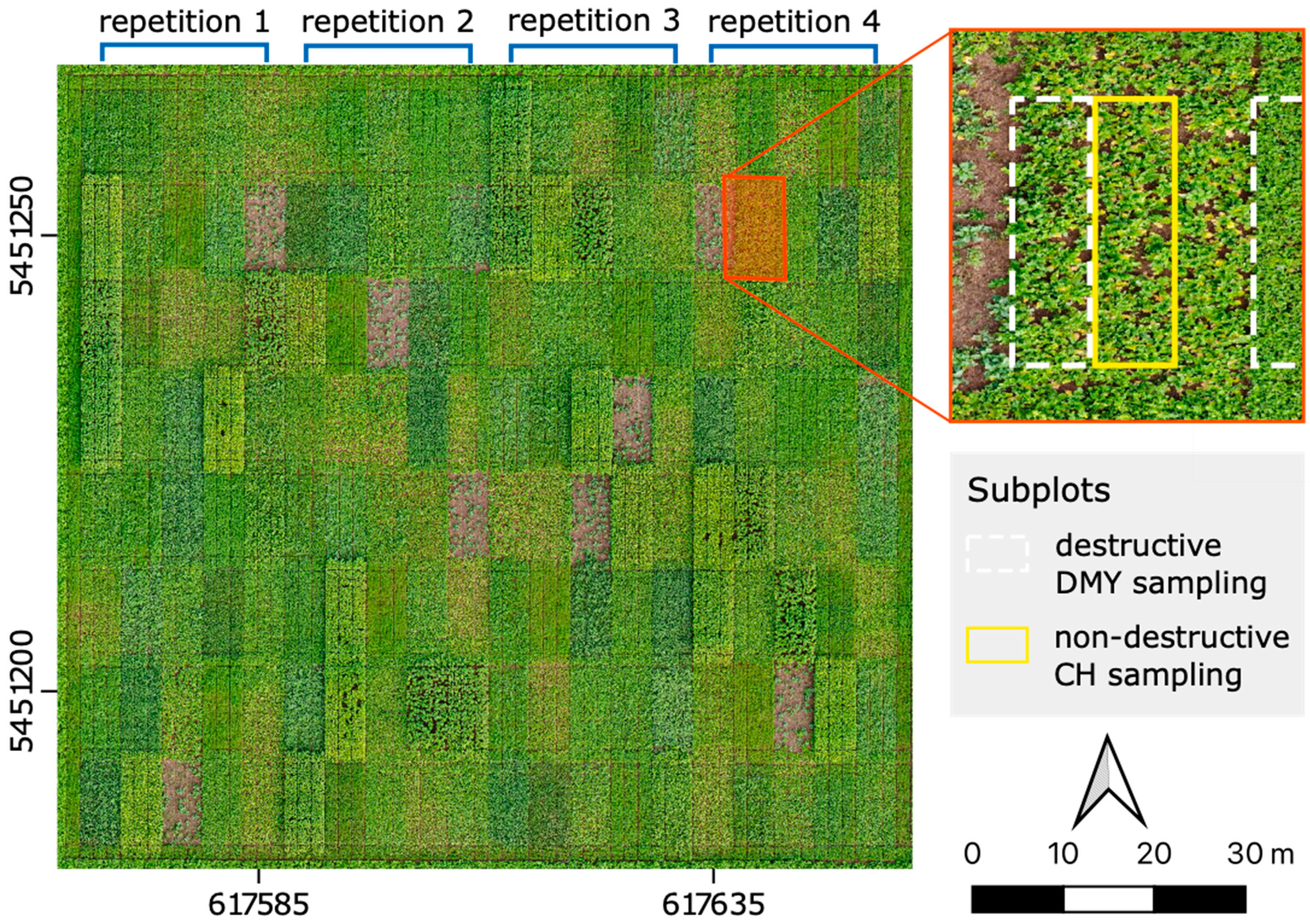
The study was conducted on a field at Landwirtschaftliche Lehranstalten Triesdorf in Weidenbach, Middle Franconia, Germany (49°12′9.0504″N, 10°36′51.7716″E, 436 m above sea level). The predominant soil was sandy loam. The Stagnic-Cambisols developed from shallow loess over in-situ weathered sandstone–claystone (Keuper). An average temperature of 9.0 °C and annual precipitation of 648 mm (long-term mean, 2010–2019) characterize the cool–temperate climate. Cover crops (CC) were sown on 23 August 2019 in 1.5 m × 7.5 m plots with a mechanical plot drill and a real-time kinematic (RTK)-steered tractor after soil preparation with a cultivator. The preceding crop was winter barley. No pesticides and fertilizers were applied. Precipitation for the growth period from sowing at the end of August to harvest for biomass sampling at the beginning of November was 113 mm. The field trial comprised 40 treatments, of which 37 were included in the study (one was bare fallow as control, and two others were harvested before height measurements). Each core plot was neighbored by two edge plots to avoid edge effects. Treatments were replicated four times and arranged in a randomized complete block design (Figure 2).
Treatments include pure stands representing different CC species (Table 1) or mixtures of several CC species. Additionally, for mustard and oil radish, treatments with systematically increased seed rates from 12.5%, 25%, 50%, 100%, and 200% of the typical seed density of 250 grains m−2 for mustard and 180 grains m−2 for oil radish (Table 1) were established. The seed rate of the individual species included in the 23 tested mixtures was determined by dividing the regular seed density of these species (Table 1) by the total number of species in the mixture. The total number of mixtures was split into 11 dual mixtures, 10 triple mixtures, and 2 complex mixtures comprising all tested species with and without mustard.

2.2. Data Acquisition

Two missions with two different UAV-based camera systems were carried out on 15 November 2019 at the end of the vegetation period to capture images of the cover-crop canopies (Table 2). Overcast weather conditions prevented direct sunlight and shadows while missions were executed. The main differences between the systems were the sensor resolutions and the flight altitudes resulting in the ground sample distance varying by a factor of 10. Low-resolution (LR) images were taken by a multispectral sensor (Parrot SEQUOIA+, Paris, France) with a 1.2-megapixel (MP) sensor resolution firmly mounted on a quadrocopter (Parrot Bluegrass, Paris, France). Another quadrocopter (DJI Mavic Air, Shenzhen, China) with a gimbal-mounted RGB-Camera with 12.3 MP (DJI FC2103, Shenzhen, China) was used to capture the high-resolution (HR) images. Mission planning was accomplished with ParrotFields and Pix4Dcapture (both Pix4D SA, Lausanne, Switzerland), respectively. In total, 78 LR and 308 HR images were captured during the two missions (Table 2).
Manual CH was assessed one week before flight missions. According to the definition of canopy height in the publication, manual CH was not calculated from the plant height of single plants but with a square rising plate of 0.06 m2 (0.21 × 0.30 m) lying on the crop stand with a ruler at a precision of 0.01 m [40]. The measurements in each core plot were repeated twice with a distance of 3–4 m between sampling points. The CH value from the ruler (CHRuler) represents the mean of both measured values for each plot.
On 6 November 2019, one of the edge plots for each repetition was harvested with a forage plot harvester at a stubble height of 5 cm. The fresh matter weight was quantified via the harvester for the whole plot. Biomass samples were dried at 60 °C to a constant weight (min. 48 h) to determine dry matter content and dry matter yield (DMY).

2.3. Data Processing of Remote-Sensing Images

Processing of image data from both missions was done in the same workflow. To generate three-dimensional (3D) point clouds and georeferenced digital surface models (DSM) from the captured images, the structure-from-motion (SfM) approach was applied by utilizing the software Agisoft Metashape v. 1.6.2 Professional Edition (Agisoft LLA, St. Petersburg, Russia). SfM is a method for obtaining 3D information by superimposing images from different positions using parallax [41]. After images had been imported, the coordinate system was converted to WGS 84/UTM zone 32N (EPSG::32632), and image quality was estimated with the built-in algorithm from Metashape. Nearly all LR images had an image quality value of 0, meaning that the algorithm classifies the image quality as insufficient. The rating results from the comparatively low resolution of the LR images, but SfM calculates the distance for each pixel, and the optical image quality hardly affects these results. All HR images had an image quality value greater than 0.68 due to the increased resolution [42]. Before alignment, HR images from the DJI camera were pre-calibrated by applying values for all fixed parameters obtained from lens calibration with the chessboard method to avoid a curvature effect. Furthermore, altitude information for images captured by the DJI camera was changed from the relative altitude referring to the starting point to absolute altitude by adding the mean ground altitude of the experimental area to the EXIF information with a Python script [43]. Alignment was performed with the highest accuracy, reference preselection, and a key point limit and tie point limit of 40,000 and 4000, respectively. Adaptive camera model fitting was enabled. In the Quantum Geographical Information System (QGIS 3.4.8, QGIS Development Team, Raleigh, NC, USA), 40 virtual ground control points (GCPs) were created by selecting edges of the plot polygons, which were distributed over the experimental area. The plot polygons were sourced from the plot trial planning software MiniGIS which initially served for path planning of the sowing operation (geo-konzept GmbH, Adelschlag, Germany). Since plots were sown with an RTK-steered tractor, it was assumed that plot edge positions in the field had high accuracy. To provide GCPs with altitude information, a digital terrain model (DTM) generated by a laser scan survey (Bayerische Vermessungsverwaltung 2017) was used to assign altitude values to each marker. GCPs were imported to Metashape for each marker, and at least four images were linked and verified. The software can minimize reprojection errors and reference coordinate misalignment errors by adjusting camera parameters. The georeferenced and optimized sparse point cloud was then transformed into a dense point cloud in ultra-high quality (processing original scaled photos without downscaling) and mild depth filtering to preserve all details in the canopy structure. The last step in Metashape was to generate a DSM from a dense cloud with disabled interpolation. DSM was exported as a tagged imaged file format file (TIFF) and imported to QGIS, where the DSM was transformed into a canopy height model (CHM). In the DSM, plots with a buffer of 0.3 m and the areas in between the plots were masked. As a result, only those areas remained where the cover crops were mowed during harvest. Therefore, only stubbles were present in those regions, and most of the area was ground. The masked regions of the DSM were interpolated with inverse distance weighted interpolation to obtain a DTM. The CHM was calculated by subtracting DTM from DSM [22] (Figure 1). Mean CH values from LR imaging (CHLR) and HR imaging (CHHR) were calculated for each plot using R statistics software version 4.0.3 (R Foundation for Statistical Computing, Vienna, Austria) and package raster version 3.6-3 [44]. The plot polygon data from MiniGIS were buffered by −0.3 m to avoid edge effects and insufficient georeferencing.

2.4. Statistical Analysis

Statistical Analysis was performed using R programming language version 4.0.3 (R Foundation for Statistical Computing, Vienna, Austria). Reduced major axis (RMA) regression (also called standard major axis or SMA regression), which is a Type-II regression model, is suggested to be used instead of the ordinary least-squares model (Type-I regression model) [45]. Because it is unclear which variable would be considered the independent or the dependent variable, a bivariate relationship must be defined. The comparison of CHRuler and CHLR compares two measuring methods where no variable could be considered independent or dependent. For this reason, the linear relationship of CHRuler and CHLR was tested by an RMA regression. Since Pearson correlations were significant, RMA regression was used to calculate the adjusted coefficient of determination (R2) and root mean square error to compare the different datasets.
Before the paired t-test was performed, pairwise differences between CHRuler, CHLR, and CHHR were tested for Gaussian distribution with the Shapiro–Wilk test. As the assumption of normal distribution was not fulfilled, the variables were square-root-transformed.

3. Results

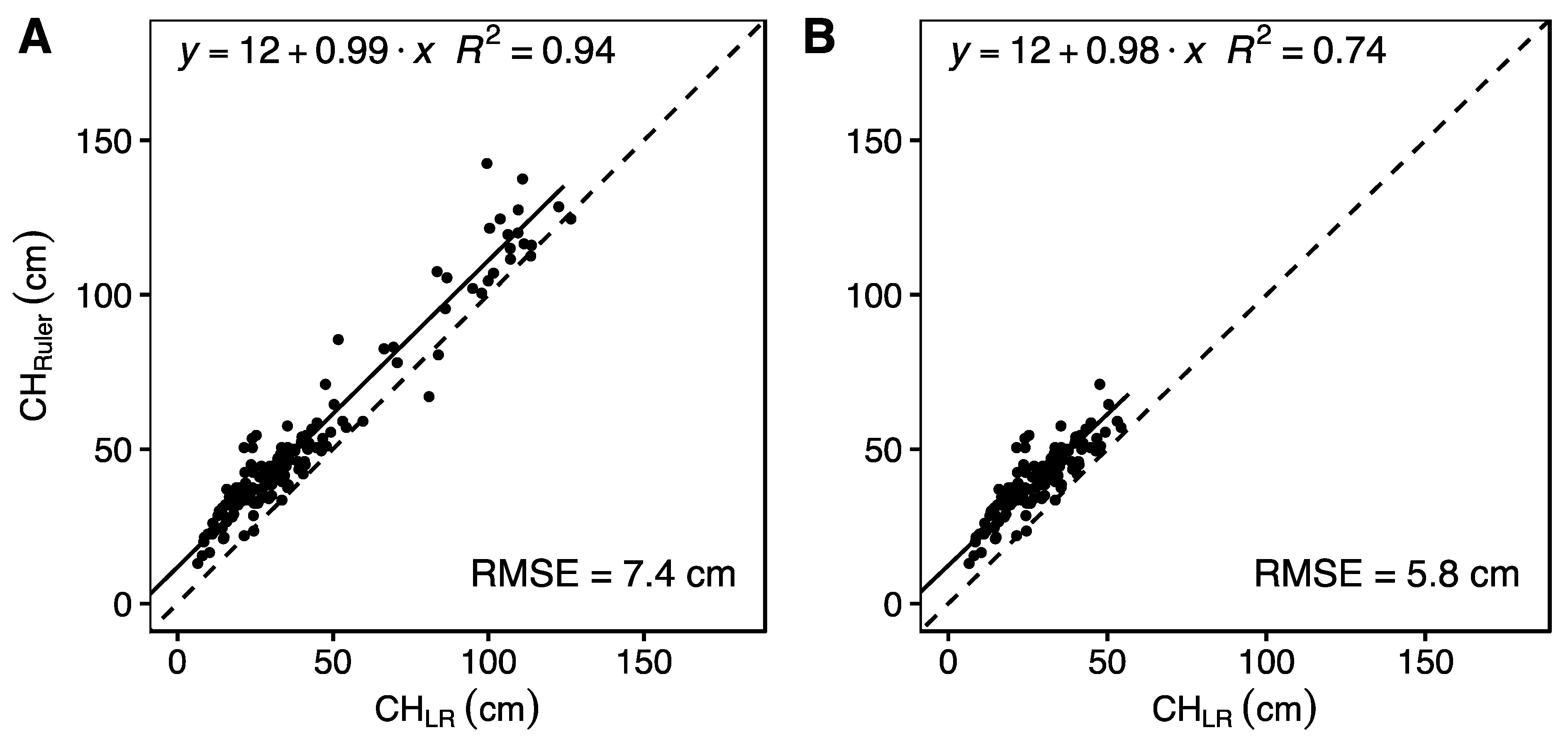
To verify if UAV-based RGB images can provide a sufficient foundation to estimate the crop height of diverse CC mixtures under field conditions, a field trial was conducted with pure and mixed stands of six commonly used cover-crop species (Table 1). Mean CH for CC plots varied in a span of 13 to 143 cm measured by a ruler-based method (CHRuler) and 7 to 127 cm calculated on the base of LR RGB images (CHLR). Nearly all treatments containing mustard in pure stand or mixtures showed a CHLR greater than 60 cm. It can be explained by the rapid growth rate and the early occurrence of the jointing stage of mustard plants growing under long-day conditions. Thus, mustard reaches the longitudinal growth stage much earlier than other tested species. A linear regression analysis of CHRuler and CHLR showed an R2 of 0.94 and an RMSE of 7.4 cm (Figure 3A). Compared with the other tested CC plants, mustard had a significantly higher crop height (Table A1). Thus, it represented extreme values in the dataset suspected of biasing the regression model. All mustard treatments were excluded from a second linear regression analysis to eliminate possible bias by mustard plants, and their impact on the regression model was examined (Figure 3B). The R2 of all mustard-free treatments dropped to 0.74 compared to the R2 of 0.94 when mustard treatments were included, indicating the strong impact of tall mustard plants on this value. Meanwhile, the model parameters of the regression and RMSE were nearly unaffected.
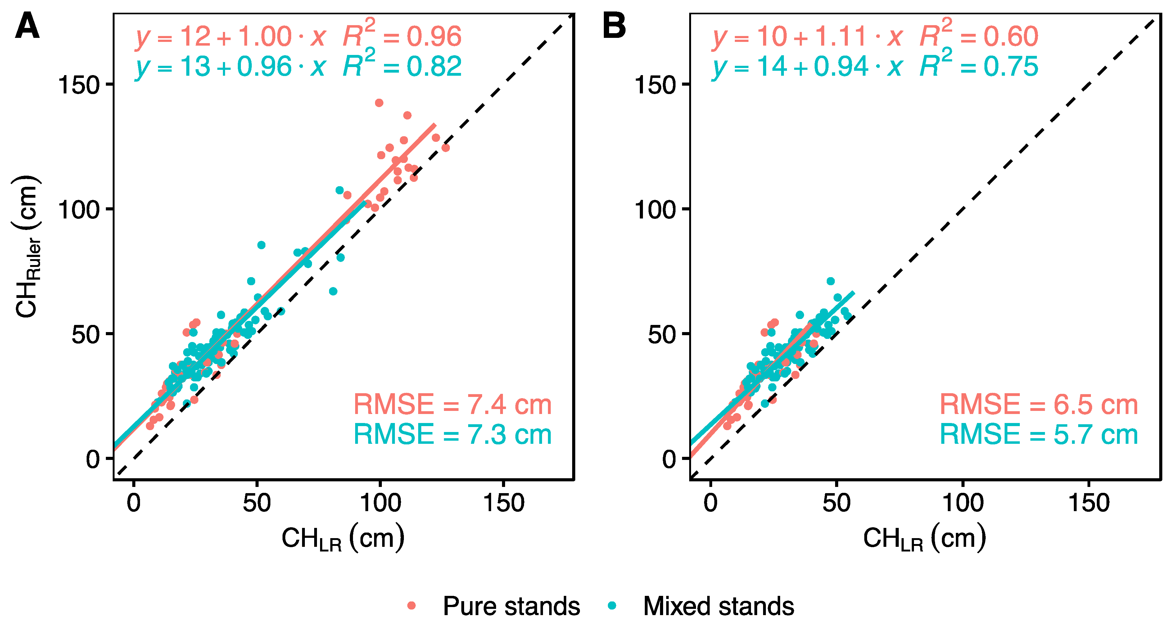
Additionally, it was evident that the ruler-based measurements of mean CHs led to approximately 12 cm higher values than the UAV-based measurements in CC stands (Figure 4A,B). Both datasets, containing mustard or not, showed slopes close to 1.0. Thus, the UAV-based measurement constantly underestimated plant height, whether the stands were relatively small or high. Instead of the mean, the 90th or 99th percentile was also used to optimize the regression model. As expected, comparing the ruler method with the percentiles led to decreased intercepts (8 cm and 5 cm) with consistent coefficients of determination. However, the slopes decreased substantially (0.89 and 0.86), and the RMSE decreased slightly (6.8 and 7.3) (Figure A1). The intercept between the two methods can also be explained by the high variance of individual plant height in CC mixtures or even small bare areas without plant cover, which were captured in more detail by the UAV-based approach than by the ruler method. Small bare areas can be frequently observed under field conditions due to inhomogeneous seed distribution in the seed furrow, treatments with low seeding rates, or various germinating conditions. CCs in the present field experiment were grown in either pure stands as single species or mixed stands composed of two to six species. Therefore, in mixtures, different species with different habitus grew side by side, leading to probably uneven canopies due to CC stands consisting of plants with different heights. In contrast, pure stands show more even canopies. To investigate if the heights of CC mixtures determined via RGB images and ruler-based measurements are influenced differently by pure stands or mixtures, the dataset was clustered into pure and mixed CC stands, and linear regression models were applied (Figure 4A). The plot’s highest and lowest mean CHs were found in pure stands. For example, plots with mustard as a single species showed the highest values, while mustard in mixtures showed lower mean CHs (Table A2). R2 was slightly higher for pure stands (R2 = 0.96) and was substantially lower for mixed stands (R2 = 0.82) than the entire dataset, as shown in Figure 4A. No change was observed for RMSE values in the entire dataset (Figure 4A). In the dataset, without mustard-containing treatments, RMSE values changed inversely: pure stands increased to 6.5 cm, and mixtures decreased to 5.7 cm (Figure 4B). However, R2 was lower for pure stands (R2 = 0.6) and slightly higher for mixed stands (R2 = 0.75) than in the analysis shown in Figure 4B. Interestingly, the regression slope of the pure stands without mustard-containing treatments was steeper than 1.0, indicating that clustering data in pure and mixed stands did not meet the expectation of a reasonable explanation for deviations between the two methods (Figure 4B).
The greater R2 of the mixtures compared to pure stands in the dataset without mustard refutes the idea that heterogeneous mixtures could cause discrepancies between the two height determination methods (Figure 4B). The absolute height offset cannot be explained by this either. Nevertheless, canopy shape is determined by the used species and different combinations of species in mixtures. Accordingly, more than the subdivision in pure and mixed stands was needed.
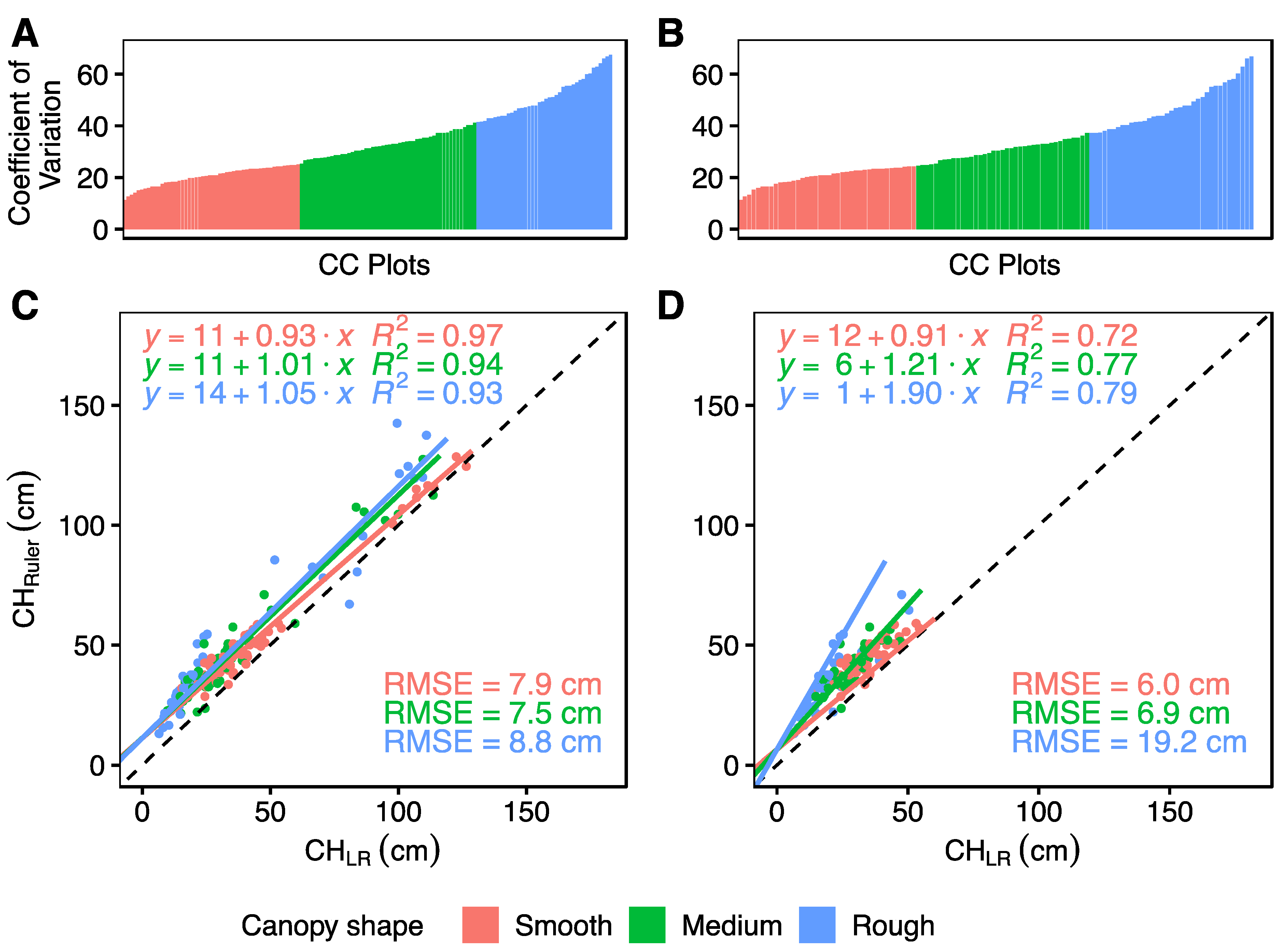
A suitable method to describe canopy structure could be the relative deviation of approximately 4500 CH measurements per plot. The coefficient of variation (CV) was computed using data from the LR UAV mission for each plot. CV varied from 7.8 to 67.1%. Subsequently, the plots were classified into three clusters of similar sample sizes. Sample sizes were not equal due to the filtering of treatments not included in the analysis. They were named “smooth” for the cluster containing treatments showing the lowest CVs, “medium” for the intermediate, and “rough” for the cluster with the highest CV values (Figure 5A,B).
The regression between CHLR and ruler-based CH fitted best to the cluster containing smooth canopy shapes for the entire dataset. This results in the highest R2 (0.97) and lowest RMSE for smooth canopy shapes (Figure 5C). Even when the mustard-containing treatments were removed, the highest R2 of the three clusters was observed in the “smooth” cluster (0.74) (Figure 5D). The lowest R2 in both datasets was found in the “medium” cluster. Although the difference in RMSE between canopy shapes was low, the R2 showed apparent differences. Especially in the “smooth” cluster, the regression slope was nearly 1.0, even without the mustard treatments causing high canopies (Figure 5C,D). The regression slope of “medium” and “rough” canopy shapes and the RMSE of “rough” canopy shape showed increased values in the dataset without mustard (Figure 5D) and thus remarkably deviations compared to the entire dataset (Figure 5D).
The greatest deviations between ruler-based and UAV methods occurred in CC plots with rough canopies, indicated by a high coefficient of variance. A possible explanation could be the size of the measured area (resolution) and the number of repeated measurements within a plot. During increasing resolution, the number of repeated measures in CC stands with smooth canopies does not result in more considerable changes in mean CH than in rough canopies. A comparison between the LR and HR mission results was visualized to evaluate the impact of increasing the resolution and the number of measurements per plot.
For each smooth and rough canopy, a CC stand with a high and a low CH was selected, and a profile of the CH in a transect of 800 cm was plotted. The Oil radish and Egyptian clover mixture represents the smooth and low-rise canopy (Figure 6A). In contrast, the rough and low-rise canopy (Figure 6C) is represented by a pure stand with Oil radish and halved seed density (the same as in a mixture of Oil radish and Egyptian clover). A pure mustard CC with a seed density of 125 seeds m−2 had a smooth and high-rise canopy (Figure 6B), whereas the reduced density of only 31 mustard seeds m−2 showed a rough and high-rise canopy (Figure 6D). In the smooth and low-rise canopy (Figure 6A), the increase in image resolution did not have a remarkable effect on mean CH but showed a few more details of the canopy structure. In contrast, higher resolution and sampling rates are more evident in the rough and low canopy (Figure 6C). In the high-rise and smooth canopy (Figure 6B), it can be recognized that the more detailed canopy structure, derived from the HR mission, mainly reveals spots in the canopy that are lower than in the LR CH model. This results in a lower mean CH of the HR-image-derived CH model. In the high-rise and rough canopy (Figure 6D), these effects are evident. The CC stand with strongly reduced mustard seed density was unable to achieve a closed canopy and thus left some open spots in the canopy where the soil was uncovered from the mustard shoot biomass. In the CHLR model, some little dents in the canopy could be interpreted only as hints of these spots in bare soil, while they can be detected in the canopy profile of CHHR.
The ruler-based method leads to higher mean CH values than the UAV method for all tested canopy structures, whereby the HR mission provides lower CH values than the LR mission. The most apparent differences in mean CH between the ruler and UAV method could be observed in rough CC canopies (Figure 7). For each examined canopy property, differences in mean CH values between the three applied methods were significant (paired sample t-test of square-root-transformed data, p < 0.05). For smooth canopies, the t-test could not be performed to compare CHLR and CHHR due to the not-normally distributed difference between paired values. Mustard-containing CC stands were excluded for the same reason.
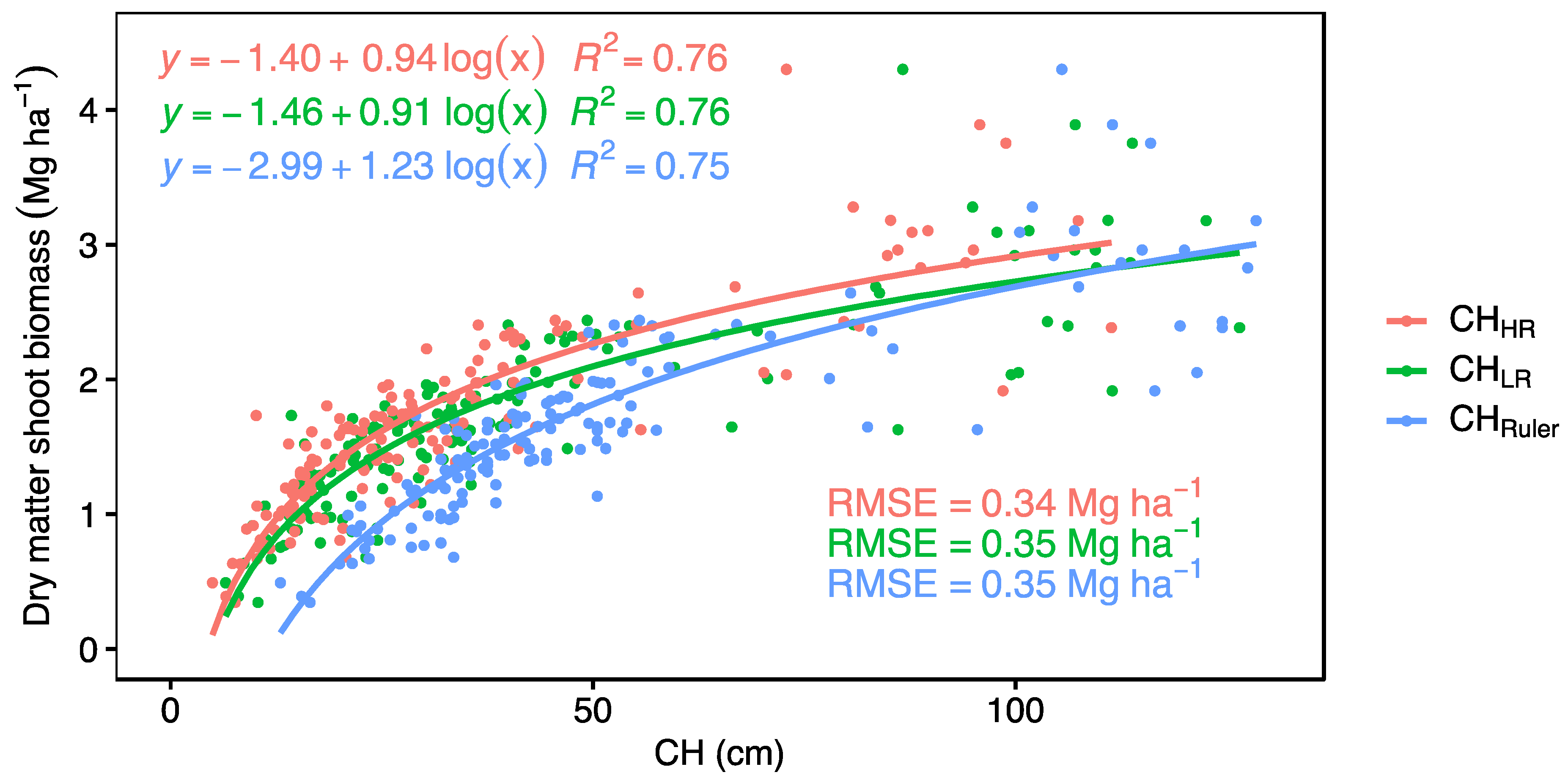
Regression models were fitted to answer the initial question of whether the biomass of cover crops is predictable by CH determined with UAV-based RGB imaging (Figure 8). Dry matter shoot biomass of the investigated cover crops yielded between 0.34 and 4.3 Mg ha−1. Logarithmic relationships between the measures were found, with an R2 = 0.76 for the HR and LR RGB imaging and 0.75 for the ruler method. As expected, the intercept of the HR model was lower than the intercept of the LR model and even lower than the ruler model. However, slight differences were found, and the RMSE was nearly identical for the three models (Figure 8).

4. Discussion

At first glance, calibrating sensor data with measured data is a straightforward approach and commonly provides the basis for remote sensing. Nevertheless, calibrating dimensionless data needs reliable in-situ data—the so-called ground truth.

4.1. Plant Height or Canopy Height?

Comparing our results to the literature first raised the question of whether the compared studies aimed to measure plant height or CH. When publications focused on matching “ground truth measurements”, top percentiles of height values were used to describe CH [46,47]. On the contrary, if the focus was on estimating above-ground biomass, mean height values were used [48,49]. According to the definition implemented in the introduction, CH includes the surface of the crop cover, even if it is not formed by apical plant parts. The uncovered ground is also included in the CH with height values of 0 (Figure 1). This definition is necessary because the present study deals with pure CC stands and diverse CC mixtures containing plant species with contrasting shoot morphology and different seeding rates, resulting in more or less dense plant stands and, in extreme cases, leading to gaps in the plant stands.
Hence, an ideal method to quantify CH for biomass prediction is to average the crop stand surface height, including tops and gaps. In the case of plant height, only the highest parts of the individual plant are taken into account, while in the case of CH, lower parts of a plant are also taken into account if they form the surface of the plant cover. Determination of canopy tops assumes a uniform canopy, which is not provided under poorly established or lodged crop stands [31]. Thus, the top percentiles of height values will overestimate the actual CH. Especially in mixed plant stands, showing vertical niche differentiation in above-ground plant parts, conventional methods such as the ruler-based method can only determine the plant height of the tallest plants in a stand. Thus, this inevitably overestimates the actual mean height of the combined individual plants in a stand. Due to the definition, plant height is insufficient to consider plant density, gaps in crop stands, and non-apical plant parts, which nevertheless form the surface of the plant cover. Therefore, a sufficient estimate of above-ground biomass would also not be possible using this measure. Using a ruler to measure CH under practical conditions is described as subjective by Scotford and Miller [50]. In order to obtain more objective data when using the ruler method, a rising plate meter was introduced. The rising plate meter combines height and density into one measure [51]. Since the rising plate meter and UAV measurement address CH, a close correlation is expected between the methods. Therefore, the UAV method should be an adequate substitute for labor-intensive hand measurement.

4.2. Is Ground Truth the Truth?

CH provided by UAV imagery, on average, was 12 cm (LR) and 18 cm (HR) lower than CH provided by the rising plate meter (Figure 7). Similar observations were found in previous studies for CCs [27] but also for a range of other crops such as grassland [48,49,52,53], barley [22], wheat [54], maize [55], and oilseed rape [32]. Our study and the previous studies had in common that the number of recorded data points for manual measurements was very limited compared with the number of data points recorded by UAV imagery in the same area. While manual measurements represent only the top of the plants and cover only a limited area of the plot, the UAV method also considers the lower parts of the plants or even the bare soil in the case where the crop stand is not dense or well established [22]. Consequently, the mean height from the UAV must be lower than the mean height from manual measurement. Nevertheless, R2 between CHLR and CHRuler was very high (Figure 3). In similar studies, R2 values ranging from 0.40 to 0.92 were found. However, several points should be noted when comparing the results of different studies. Studies investigating a single crop, such as barley, wheat, perennial ryegrass, or maize, achieved an R2 value between 0.90 and 0.92 [22,54,55,56], whereas studies dealing with multiple crop species in grassland or cover crops achieved lower R2 values [27,49,57]. The level of R2 also depends on whether means or top quantiles were used to compare UAV height with ruler height. Therefore, in some studies, the percentile showing the lowest deviation from manual measurements was analyzed [27,29,31,55]. In this context, the R2 of regression models from the present study, which investigated the mean height of multiple (mixed) CC species in different seed densities, shows high accuracy. Mustard plants grew significantly higher than the other species, resulting in not-normally distributed data and thus influenced R2 positively (Figure 3). A similar effect can be observed in previous studies that integrated different sampling dates into one regression model. However, these studies probably achieved normal distribution due to the same samples from different dates [29,49,56].
Measuring height in crop stands can be performed best for smooth and dense canopies, as assumed by Grenzdörffer [32]. In our results, homogeneity and density are represented by the coefficient of variation. It is clearly shown that the higher the coefficient of variation, the more deviation between the ruler and UAV method can be observed (Figure 5). In previous studies, similar findings resulted in the hypothesis that a low number of manual height measurements within a plot do not produce an accurate mean of the CH. To address this problem, Bendig et al. [22] suggested decreasing the area of the transects where height is measured to cover the canopy’s heterogeneity better. Ruyeda-Ayala et al. [52] implemented this suggestion and observed a more robust relationship for height measurements between UAV and ruler methods. Additionally, CH measurements made using conventional manual methods are often subjective because operators potentially have a different perception of what constitutes the height of the canopy [31]. Nevertheless, many studies describe manual height measurements as “ground truth” [27,28,29,52].
Therefore, the following questions arise: Can we speak of ground truth if the ruler method inadequately describes the CH due to a small number of measurements per sample area? Moreover, can ruler measurements achieve the quality of HR UAV measurements in different plant stands? The present and several previous studies provide clear hints that remote-sensing measurements of CH show increased accuracy compared to the manual ruler method. This is based on a tremendous increase in measurement number per sample area—in other words, the decrease in ground sample distance (GSD). In general, it is accepted in literature to parameterize models of dimensionless remote-sensing data by using ground measurement. However, compared to, for example, spectral data for vegetation indices, the SfM approach delivers data with a dimension from UAV images. Borra-Serrano et al. [56] investigated the altimetric accuracy of their SfM model in a range of 0–40 cm. They found an average variance value of only −0.56 cm, which is more than sufficient for CH purposes and proves the accuracy of the SfM approach. Thus, SfM photogrammetry generally determines the height of crops correctly and accurately. Therefore, we assume that the discrepancies between the CHs derived from the manual ground measurements and the UAV images are mainly due to the inaccuracy of the manual ground measurements caused by a too-low number of measurements in a too-inhomogeneous canopy, as shown by the results in Figure 5. Consequently, validation of CH derived from UAV imagery with conventional measured ground data does not make sense because the ground data does not match the accuracy of the UAV imagery [58].
Suppose UAV imagery can determine the mean CH more accurately due to the increased resolution and number of measurements than manual ground measurement. In that case, increasing image resolution or, more specifically, decreasing GSD must lead to an even more precise CH mean. A comparison of CH profiles from UAV imagery shows that a lower GSD reveals more details of crop canopies. Insights are primarily given to gaps and areas with lower heights in sparse and inhomogeneous canopies (Figure 6). Further, using the SfM approach, mean CH decreases if the resolution of the CH model increases (Figure 7) because the upper parts of the canopy are overestimated compared with the lower parts. To determine CH via SfM photogrammetry, it can be recommended to lower the GSD for sparse and inhomogeneous canopies to obtain reliable results, which was also found by Hämmerle et al. [46].

4.3. Predicting Biomass Yield by Canopy Height

The observed shoot biomass of cover crops was between 0.34 and 4.3 Mg ha−1, which matches the findings of other studies under similar framework conditions [59,60,61]. The value of R2 = 0.76 from regression analysis shows that CH is well-suited as a predictor for the DMY of cover crops (Figure 8). Other studies predicted DMY by CH with higher accuracy for winter wheat (R2 = 0.78) [24] and spring barley (R2 = 0.82) [22] grown as monocultures. Studies investigating different species reported slightly lower accuracy for clover–grass (R2 = 0.75) and lucerne–grass mixes (R2 = 0.64) [49]. Roth and Streit [27] analyzed different cover crops as monocultures and found an R2 = 0.58. Nevertheless, they could increase R2 to 0.74 for selected species with correlation coefficients above 0.6. One reason for this discrepancy in more heterogeneous canopies for mixed crops is presumed to be due to different coverage or morphological differences among various species [49,56]. Indeed, the accuracy of our regression analysis was better for pure stands (R2 = 0.72) than for mixtures (R2 = 0.72), but this could also be due to further-apart extreme values in the dataset of pure stands. The hypothesis is countered by a comparison of regression analysis with our classification in smooth (R2 = 0.68), medium (R2 = 0.80), and rough canopy shapes (R2 = 0.80) (Table 3).
Among the three methods used to determine CH in this study, no apparent differences in the accuracy of the regression analysis to predict DMY were found. A possible explanation is that CH and DMY were determined in different subplots of a 33.75 m2 homogeneously cultivated plot. Nevertheless, analyzing destructive and non-destructive measures in different areas of a plot is common practice. As mentioned previously, the CH measure incorporates plant height and plant density, therefore representing a volumetric measure. Especially for homogenous crops like wheat, the volume is highly correlated with the above-ground biomass [62]. However, estimating biomass with reasonable accuracy based on volume alone is impossible if plant allometry (i.e., relationships based on plant shape, height, size, age, or structure) is ignored [63]. Since different CC species show different allometric properties, the dependence between CH and DMY is variable. Therefore, the accuracy of the CH value plays only a minor role in estimating DMY. To summarize, cover-crop biomass can be well predicted by CH, and data collection with UAV could be a suitable hands-on method for farmers. Assuming that biomass nitrogen concentration depends on the proportion of legumes and non-legumes in cover-crop mixtures, farmers could also calculate nitrogen uptake and consider the data collected for fertilizer requirements of subsequent crops. A regression model for nitrogen uptake of cover crops could also be improved by incorporating further remote-sensed data, as shown by Lu et al. [55] or Holzhauser et al. [61].

5. Conclusions

The study investigates CH measurement of different cover-crop species grown as pure or mixed stands using UAV images processed with SfM photogrammetry. We presented a clear definition for CH which differs from plant height.
Plant breeders often require plant height to be characterized and are more interested in information on individual plants from homozygous varieties than whole crop stands of possibly mixed species. The SfM method delivers dimensioned remotely sensed data and, in contrast to non-dimensioned data, does not necessarily need to be validated by manual height measures. On the one hand, the analysis showed that decreased ground sample distance led to more accurate CH measurements, especially in sparse and inhomogeneous crop stands. On the other hand, the agreement between manual in-situ measured and remotely sensed UAV-imagery-derived CH was lower if crop stands were not uniform. Hence, we concluded that manual measurement, often entitled “ground truth”, cannot determine CH with sufficient accuracy due to much fewer measurements per sample area and thus cannot serve as validation for CH derived from HR UAV imagery. For evaluating the CH of plant stands on arable fields and field trials for crop production, we recommend preferring SfM photogrammetry, even with comparably low ground sample distance. Compared with manual ground measurement, this method is more objective, accurate, and less time-consuming for large survey areas, especially in inhomogeneous crop stands. Spatial differences can be captured and developed for site-specific applications in precision agriculture.

Author Contributions

Conceptualization, R.K. and B.B.; methodology, R.K., P.O.N. and B.B.; formal analysis, R.K.; investigation, R.K. and B.B.; data curation, R.K.; writing—original draft preparation, R.K.; writing—review and editing, P.O.N. and B.B.; visualization, R.K.; supervision, P.O.N. and B.B.; project administration, B.B.; funding acquisition, B.B. All authors have read and agreed to the published version of the manuscript.

Funding

This work was supported by the German Federal Ministry of Education and Research [grant number 031B0507D–CATCHY].

Data Availability Statement

The data presented in this study are openly available in the Zenodo archive at the following DOI: https://doi.org/10.5281/zenodo.7713341 (Kümmerer, 2023).

Acknowledgments

This work is part of the BonaRes (Soil as a Sustainable Resource for the Bioeconomy) project CATCHY (Catch-cropping as an agrarian tool for continuing soil health and yield increase). We are grateful to David Eder and Stefan Uhl for technical support and to Tristan Billmann and Max Erath for assistance with measurements.

Conflicts of Interest

The authors declare no conflict of interest.

Appendix A

Table A1. Comparison of mean canopy height derived from low-resolution UAV-mission (CHLR) of the different species grown in the field experiment, standard error (SE), and compact letter display (CLD) indicating significant differences among the species according to Tukey’s test at p < 0.05).
SpeciesCHLRSEnCLD
Oil Radish11.501.884a
Field Pea23.131.884b
Egyptian Clover23.541.884b
Bristle Oat33.251.884c
Phacelia39.051.884c
Mustard106.961.884d
Figure A1. Linear relationship between canopy height from low-resolution UAV mission calculated from (A) 90th percentile (CH0.9) and (B) 99th percentile (CH0.99) and manual height measurement with a ruler-based method (CHRuler) of cover-crop treatments, n = 148.
Remotesensing 15 01520 g0a1
Table A2. Comparison of mean canopy height derived from low-resolution UAV-mission (CHLR) between the pure stand cover crops and cover crop mixtures, standard error (SE), and compact letter display (CLD) indicating significant differences among the treatments according to Tukey’s test at p < 0.05).
Cover Crop TreatmentsCHLRSEnCLD
Pure stands33.902.9956a
Mixtures50.893.8392b

References

  1. Blanco-Canqui, H.; Shaver, T.M.; Lindquist, J.L.; Shapiro, C.A.; Elmore, R.W.; Francis, C.A.; Hergert, G.W. Cover Crops and Ecosystem Services: Insights from Studies in Temperate Soils. Agron. J. 2015, 107, 2449–2474. [Google Scholar] [CrossRef] [Green Version]
  2. Gentsch, N.; Boy, J.; Batalla, J.D.K.; Heuermann, D.; von Wirén, N.; Schweneker, D.; Feuerstein, U.; Groß, J.; Bauer, B.; Reinhold-Hurek, B.; et al. Catch Crop Diversity Increases Rhizosphere Carbon Input and Soil Microbial Biomass. Biol. Fertil. Soils 2020, 56, 943–957. [Google Scholar] [CrossRef]
  3. Chahal, I.; Vyn, R.J.; Mayers, D.; van Eerd, L.L. Cumulative Impact of Cover Crops on Soil Carbon Sequestration and Profitability in a Temperate Humid Climate. Sci. Rep. 2020, 10, 13381. [Google Scholar] [CrossRef] [PubMed]
  4. Alvarez, R.; Steinbach, H.S.; de Paepe, J.L. Cover Crop Effects on Soils and Subsequent Crops in the Pampas: A Meta-Analysis. Soil Tillage Res. 2017, 170, 53–65. [Google Scholar] [CrossRef]
  5. Chahal, I.; van Eerd, L.L. Evaluation of Commercial Soil Health Tests Using a Medium-Term Cover Crop Experiment in a Humid, Temperate Climate. Plant Soil 2018, 427, 351–367. [Google Scholar] [CrossRef]
  6. Heuermann, D.; Gentsch, N.; Boy, J.; Schweneker, D.; Feuerstein, U.; Groß, J.; Bauer, B.; Guggenberger, G.; von Wirén, N. Interspecific Competition among Catch Crops Modifies Vertical Root Biomass Distribution and Nitrate Scavenging in Soils. Sci. Rep. 2019, 9, 11531. [Google Scholar] [CrossRef] [PubMed] [Green Version]
  7. Hunter, M.C.; Schipanski, M.E.; Burgess, M.H.; Lachance, J.C.; Bradley, B.A.; Barbercheck, M.E.; Kaye, J.P.; Mortensen, D.A. Cover Crop Mixture Effects on Maize, Soybean, and Wheat Yield in Rotation. Agric. Environ. Lett. 2019, 4, 180051. [Google Scholar] [CrossRef]
  8. Martin, R.C.; Astatkie, T.; Cooper, J.M.; Fredeen, A.H. A Comparison of Methods Used to Determine Biomass on Naturalized Swards. J. Agron. Crop. Sci. 2005, 191, 152–160. [Google Scholar] [CrossRef]
  9. Punalekar, S.M.; Verhoef, A.; Quaife, T.L.; Humphries, D.; Bermingham, L.; Reynolds, C.K. Application of Sentinel-2A Data for Pasture Biomass Monitoring Using a Physically Based Radiative Transfer Model. Remote Sens. Environ. 2018, 218, 207–220. [Google Scholar] [CrossRef]
  10. Murphy, W.M.; Silman, J.P.; Barreto, A.D.M. A Comparison of Quadrat, Capacitance Meter, HFRO Sward Stick, and Rising Plate for Estimating Herbage Mass in a Smooth-stalked, Meadowgrass-dominant White Clover Sward. Grass Forage Sci. 1995, 50, 452–455. [Google Scholar] [CrossRef]
  11. Fehmi, J.S.; Stevens, J.M. A Plate Meter Inadequately Estimated Herbage Mass in a Semi-Arid Grassland. Grass Forage Sci. 2009, 64, 322–327. [Google Scholar] [CrossRef]
  12. O’Donovan, M.; Dillon, P.; Rath, M.; Stakelum, G. A Comparison of Four Methods of Herbage Mass Estimation. Ir. J. Agric. Food Res. 2002, 41, 17–27. [Google Scholar]
  13. Weiss, M.; Jacob, F.; Duveiller, G. Remote Sensing for Agricultural Applications: A Meta-Review. Remote Sens. Environ. 2020, 236, 111402. [Google Scholar] [CrossRef]
  14. Jung, J.; Maeda, M.; Chang, A.; Bhandari, M.; Ashapure, A.; Landivar-Bowles, J. The Potential of Remote Sensing and Artificial Intelligence as Tools to Improve the Resilience of Agriculture Production Systems. Curr. Opin. Biotechnol. 2021, 70, 15–22. [Google Scholar] [CrossRef] [PubMed]
  15. Li, Z.; Taylor, J.; Frewer, L.; Zhao, C.; Yang, G.; Li, Z.; Liu, Z.; Gaulton, R.; Wicks, D.; Mortimer, H.; et al. A Comparative Review of the State and Advancement of Site-Specific Crop Management in the UK and China. Front. Agric. Sci. Eng. 2019, 6, 116. [Google Scholar] [CrossRef] [Green Version]
  16. Yang, C. Remote Sensing and Precision Agriculture Technologies for Crop Disease Detection and Management with a Practical Application Example. Engineering 2020, 6, 528–532. [Google Scholar] [CrossRef]
  17. Munnaf, M.A.; Haesaert, G.; van Meirvenne, M.; Mouazen, A.M. Site-Specific Seeding Using Multi-Sensor and Data Fusion Techniques: A Review. Adv. Agron. 2020, 161, 241–323. [Google Scholar] [CrossRef]
  18. Gerhards, R.; Andújar Sanchez, D.; Hamouz, P.; Peteinatos, G.G.; Christensen, S.; Fernandez-Quintanilla, C. Advances in Site-specific Weed Management in Agriculture—A Review. Weed Res. 2022, 62, 123–133. [Google Scholar] [CrossRef]
  19. Freeman, K.W.; Girma, K.; Arnall, D.B.; Mullen, R.W.; Martin, K.L.; Teal, R.K.; Raun, W.R. By-Plant Prediction of Corn Forage Biomass and Nitrogen Uptake at Various Growth Stages Using Remote Sensing and Plant Height. Agron. J. 2007, 99, 530–536. [Google Scholar] [CrossRef] [Green Version]
  20. Yin, X.; McClure, M.A.; Jaja, N.; Tyler, D.D.; Hayes, R.M. In-Season Prediction of Corn Yield Using Plant Height under Major Production Systems. Agron. J. 2011, 103, 923–929. [Google Scholar] [CrossRef]
  21. Han, L.; Yang, G.; Yang, H.; Xu, B.; Li, Z.; Yang, X. Clustering Field-Based Maize Phenotyping of Plant-Height Growth and Canopy Spectral Dynamics Using a UAV Remote-Sensing Approach. Front. Plant Sci. 2018, 9, 1638. [Google Scholar] [CrossRef] [PubMed] [Green Version]
  22. Bendig, J.; Bolten, A.; Bennertz, S.; Broscheit, J.; Eichfuss, S.; Bareth, G. Estimating Biomass of Barley Using Crop Surface Models (CSMs) Derived from UAV-Based RGB Imaging. Remote Sens. 2014, 6, 10395–10412. [Google Scholar] [CrossRef] [Green Version]
  23. Stanton, C.; Starek, M.J.; Elliott, N.; Brewer, M.; Maeda, M.M.; Chu, T. Unmanned Aircraft System-Derived Crop Height and Normalized Difference Vegetation Index Metrics for Sorghum Yield and Aphid Stress Assessment. J. Appl. Remote Sens. 2017, 11, 026035. [Google Scholar] [CrossRef] [Green Version]
  24. ten Harkel, J.; Bartholomeus, H.; Kooistra, L. Biomass and Crop Height Estimation of Different Crops Using UAV-Based Lidar. Remote Sens. 2019, 12, 17. [Google Scholar] [CrossRef] [Green Version]
  25. Capalbo, S.M.; Antle, J.M.; Seavert, C. Next Generation Data Systems and Knowledge Products to Support Agricultural Producers and Science-Based Policy Decision Making. Agric. Syst. 2017, 155, 191–199. [Google Scholar] [CrossRef]
  26. Atzberger, C. Advances in Remote Sensing of Agriculture: Context Description, Existing Operational Monitoring Systems and Major Information Needs. Remote Sens. 2013, 5, 949–981. [Google Scholar] [CrossRef] [Green Version]
  27. Roth, L.; Streit, B. Predicting Cover Crop Biomass by Lightweight UAS-Based RGB and NIR Photography: An Applied Photogrammetric Approach. Precis Agric. 2018, 19, 93–114. [Google Scholar] [CrossRef] [Green Version]
  28. Malambo, L.; Popescu, S.C.; Murray, S.C.; Putman, E.; Pugh, N.A.; Horne, D.W.; Richardson, G.; Sheridan, R.; Rooney, W.L.; Avant, R.; et al. Multitemporal Field-Based Plant Height Estimation Using 3D Point Clouds Generated from Small Unmanned Aerial Systems High-Resolution Imagery. Int. J. Appl. Earth Obs. Geoinf. 2018, 64, 31–42. [Google Scholar] [CrossRef]
  29. Chu, T.; Starek, M.J.; Brewer, M.J.; Murray, S.C.; Pruter, L.S. Characterizing Canopy Height with UAS Structure-from-Motion Photogrammetry—Results Analysis of a Maize Field Trial with Respect to Multiple Factors. Remote Sens. Lett. 2018, 9, 753–762. [Google Scholar] [CrossRef] [Green Version]
  30. Pérez-Harguindeguy, N.; Díaz, S.; Garnier, E.; Lavorel, S.; Poorter, H.; Jaureguiberry, P.; Bret-Harte, M.S.; Cornwell, W.K.; Craine, J.M.; Gurvich, D.E.; et al. Corrigendum to: New Handbook for Standardised Measurement of Plant Functional Traits Worldwide. Aust. J. Bot 2016, 64, 715. [Google Scholar] [CrossRef] [Green Version]
  31. Jimenez-Berni, J.A.; Deery, D.M.; Rozas-Larraondo, P.; Condon, A.G.; Rebetzke, G.J.; James, R.A.; Bovill, W.D.; Furbank, R.T.; Sirault, X.R.R. High Throughput Determination of Plant Height, Ground Cover, and Above-Ground Biomass in Wheat with LiDAR. Front. Plant Sci. 2018, 9, 237. [Google Scholar] [CrossRef] [PubMed] [Green Version]
  32. Grenzdörffer, G.J. Crop Height Determination with UAS Point Clouds. Int. Arch. Photogramm. Remote Sens. Spat. Inf. Sci. 2014, XL-1, 135–140. [Google Scholar] [CrossRef] [Green Version]
  33. Wendling, M.; Büchi, L.; Amossé, C.; Sinaj, S.; Walter, A.; Charles, R. Influence of Root and Leaf Traits on the Uptake of Nutrients in Cover Crops. Plant Soil 2016, 409, 419–434. [Google Scholar] [CrossRef] [Green Version]
  34. Sieling, K. Improved N Transfer by Growing Catch Crops—A Challenge. J. Kult. 2019, 71, 145–160. [Google Scholar] [CrossRef]
  35. Muñoz, J.D.; Finley, A.O.; Gehl, R.; Kravchenko Sasha, S. Nonlinear Hierarchical Models for Predicting Cover Crop Biomass Using Normalized Difference Vegetation Index. Remote Sens. Environ. 2010, 114, 2833–2840. [Google Scholar] [CrossRef]
  36. Xu, M.; Lacey, C.G.; Armstrong, S.D. The Feasibility of Satellite Remote Sensing and Spatial Interpolation to Estimate Cover Crop Biomass and Nitrogen Uptake in a Small Watershed. J. Soil Water Conserv. 2018, 73, 682–692. [Google Scholar] [CrossRef]
  37. Breunig, F.M.; Galvão, L.S.; Dalagnol, R.; Dauve, C.E.; Parraga, A.; Santi, A.L.; della Flora, D.P.; Chen, S. Delineation of Management Zones in Agricultural Fields Using Cover–Crop Biomass Estimates from PlanetScope Data. Int. J. Appl. Earth Obs. Geoinf. 2020, 85, 102004. [Google Scholar] [CrossRef]
  38. Chapagain, T.; Lee, E.A.; Raizada, M.N. The Potential of Multi-Species Mixtures to Diversify Cover Crop Benefits. Sustainability 2020, 12, 2058. [Google Scholar] [CrossRef] [Green Version]
  39. Finney, D.M.; Murrell, E.G.; White, C.M.; Baraibar, B.; Barbercheck, M.E.; Bradley, B.A.; Cornelisse, S.; Hunter, M.C.; Kaye, J.P.; Mortensen, D.A.; et al. Ecosystem Services and Disservices Are Bundled in Simple and Diverse Cover Cropping Systems. Agric. Environ. Lett. 2017, 2, 170033. [Google Scholar] [CrossRef]
  40. Michell, P. Value of a Rising-Plate Meter for Estimating Herbage Mass of Grazed Perennial Ryegrass-White Clover Swards. Grass Forage Sci. 1982, 37, 81–87. [Google Scholar] [CrossRef]
  41. Westoby, M.J.; Brasington, J.; Glasser, N.F.; Hambrey, M.J.; Reynolds, J.M. ‘Structure-from-Motion’ Photogrammetry: A Low-Cost, Effective Tool for Geoscience Applications. Geomorphology 2012, 179, 300–314. [Google Scholar] [CrossRef] [Green Version]
  42. Agisoft LLC. Agisoft Metashape User Manual Professional Edition; Version 1.6; Agisoft LLC: St. Petersburg, Russia, 2020. [Google Scholar]
  43. Metashape Scripts. Available online: https://github.com/agisoft-llc/metashape-scripts (accessed on 30 January 2023).
  44. Hijmans, R.J. Raster: Geographic Data Analysis and Modeling. R Package Version 3.6-3. Available online: https://CRAN.R-project.org/package=raster (accessed on 30 January 2023).
  45. Smith, R.J. Use and Misuse of the Reduced Major Axis for Line-Fitting. Am. J. Phys. Anthropol. 2009, 140, 476–486. [Google Scholar] [CrossRef] [PubMed]
  46. Hämmerle, M.; Höfle, B. Effects of Reduced Terrestrial LiDAR Point Density on High-Resolution Grain Crop Surface Models in Precision Agriculture. Sensors 2014, 14, 24212–24230. [Google Scholar] [CrossRef] [Green Version]
  47. Friedli, M.; Kirchgessner, N.; Grieder, C.; Liebisch, F.; Mannale, M.; Walter, A. Terrestrial 3D Laser Scanning to Track the Increase in Canopy Height of Both Monocot and Dicot Crop Species under Field Conditions. Plant Methods 2016, 12, 9. [Google Scholar] [CrossRef] [Green Version]
  48. Batistoti, J.; Marcato, J.; Ítavo, L.; Matsubara, E.; Gomes, E.; Oliveira, B.; Souza, M.; Siqueira, H.; Filho, G.S.; Akiyama, T.; et al. Estimating Pasture Biomass and Canopy Height in Brazilian Savanna Using UAV Photogrammetry. Remote Sens. 2019, 11, 2447. [Google Scholar] [CrossRef] [Green Version]
  49. Grüner, E.; Astor, T.; Wachendorf, M. Biomass Prediction of Heterogeneous Temperate Grasslands Using an SfM Approach Based on UAV Imaging. Agronomy 2019, 9, 54. [Google Scholar] [CrossRef] [Green Version]
  50. Scotford, I.M.; Miller, P.C.H. Combination of Spectral Reflectance and Ultrasonic Sensing to Monitor the Growth of Winter Wheat. Biosyst. Eng. 2004, 87, 27–38. [Google Scholar] [CrossRef]
  51. Sanderson, M.A.; Rotz, C.A.; Fultz, S.W.; Rayburn, E.B. Estimating Forage Mass with a Commercial Capacitance Meter, Rising Plate Meter, and Pasture Ruler. Agron. J. 2001, 93, 1281–1286. [Google Scholar] [CrossRef] [Green Version]
  52. Rueda-Ayala, V.P.; Peña, J.M.; Höglind, M.; Bengochea-Guevara, J.M.; Andújar, D. Comparing UAV-Based Technologies and RGB-D Reconstruction Methods for Plant Height and Biomass Monitoring on Grass Ley. Sensors 2019, 19, 535. [Google Scholar] [CrossRef] [Green Version]
  53. Zhang, H.; Sun, Y.; Chang, L.; Qin, Y.; Chen, J.; Qin, Y.; Du, J.; Yi, S.; Wang, Y. Estimation of Grassland Canopy Height and Aboveground Biomass at the Quadrat Scale Using Unmanned Aerial Vehicle. Remote Sens. 2018, 10, 851. [Google Scholar] [CrossRef] [Green Version]
  54. Becirevic, D.; Klingbeil, L.; Honecker, A.; Schumann, H.; Rascher, U.; Léon, J.; Kuhlmann, H. On the derivation of crop heights from multitemporal UAV based imagery. ISPRS Ann. Photogramm. Remote Sens. Spat. Inf. Sci. 2019, IV-2/W5, 95–102. [Google Scholar] [CrossRef] [Green Version]
  55. Lu, J.; Cheng, D.; Geng, C.; Zhang, Z.; Xiang, Y.; Hu, T. Combining Plant Height, Canopy Coverage and Vegetation Index from UAV-Based RGB Images to Estimate Leaf Nitrogen Concentration of Summer Maize. Biosyst. Eng. 2021, 202, 42–54. [Google Scholar] [CrossRef]
  56. Borra-Serrano, I.; de Swaef, T.; Muylle, H.; Nuyttens, D.; Vangeyte, J.; Mertens, K.; Saeys, W.; Somers, B.; Roldán-Ruiz, I.; Lootens, P. Canopy Height Measurements and Non-destructive Biomass Estimation of Lolium Perenne Swards Using UAV Imagery. Grass Forage Sci. 2019, 74, gfs.12439. [Google Scholar] [CrossRef]
  57. Lussem, U.; Bolten, A.; Menne, J.; Gnyp, M.L.; Schellberg, J.; Bareth, G. Estimating Biomass in Temperate Grassland with High Resolution Canopy Surface Models from UAV-Based RGB Images and Vegetation Indices. J. Appl. Remote Sens. 2019, 13, 034525. [Google Scholar] [CrossRef]
  58. Bareth, G.; Bendig, J.; Tilly, N.; Hoffmeister, D.; Aasen, H.; Bolten, A. A Comparison of UAV-and TLS-Derived Plant Height for Crop Monitoring: Using Polygon Grids for the Analysis of Crop Surface Models (CSMs). Photogramm. Fernerkund. Geoinf. (PFG) 2016, 2, 85–94. [Google Scholar] [CrossRef] [Green Version]
  59. Heuermann, D.; Gentsch, N.; Guggenberger, G.; Reinhold-Hurek, B.; Schweneker, D.; Feuerstein, U.; Heuermann, M.C.; Groß, J.; Kümmerer, R.; Bauer, B.; et al. Catch Crop Mixtures Have Higher Potential for Nutrient Carry-over than Pure Stands under Changing Environments. Eur. J. Agron. 2022, 136, 126504. [Google Scholar] [CrossRef]
  60. Gentsch, N.; Heuermann, D.; Boy, J.; Schierding, S.; von Wirén, N.; Schweneker, D.; Feuerstein, U.; Kümmerer, R.; Bauer, B.; Guggenberger, G. Soil Nitrogen and Water Management by Winter-Killed Catch Crops. SOIL 2022, 8, 269–281. [Google Scholar] [CrossRef]
  61. Holzhauser, K.; Räbiger, T.; Rose, T.; Kage, H.; Kühling, I. Estimation of Biomass and N Uptake in Different Winter Cover Crops from UAV-Based Multispectral Canopy Reflectance Data. Remote Sens. 2022, 14, 4525. [Google Scholar] [CrossRef]
  62. Walter, J.; Edwards, J.; McDonald, G.; Kuchel, H. Photogrammetry for the Estimation of Wheat Biomass and Harvest Index. Field Crops Res. 2018, 216, 165–174. [Google Scholar] [CrossRef]
  63. Gil-Docampo, M.L.; Arza-García, M.; Ortiz-Sanz, J.; Martínez-Rodríguez, S.; Marcos-Robles, J.L.; Sánchez-Sastre, L.F. Above-Ground Biomass Estimation of Arable Crops Using UAV-Based SfM Photogrammetry. Geocarto Int. 2020, 35, 687–699. [Google Scholar] [CrossRef]
Figure 1. Illustration of the digital surface model (blue line) following the top surface of the vegetation and the digital terrain model (brown line) following the terrain below. The red arrow indicates an example of the plant height, measured between the ground and the apical part of the plant. The pink arrow indicates an example of canopy height, measured between the ground and the visible top of the plants or the ground, where the ground is uncovered. The three yellow squares illustrate the resolution of the different methods for determining canopy height, with the ruler-based method showing the coarsest resolution and HR imaging the finest resolution.
Remotesensing 15 01520 g001
Figure 2. Aerial image of the cover-crop field trial indicating the repetitions and a scheme of the plots divided into subplots for destructive dry matter yield (DMY) sampling and non-destructive canopy height (CH) sampling.
Remotesensing 15 01520 g002
Figure 3. Linear relationship between canopy height from low-resolution UAV mission (CHLR) and manual height measurement with a ruler-based method (CHRuler) of cover-crop treatments (A) for the whole dataset (n = 148) and (B) for the dataset excluding treatments containing mustard plants (n = 120).
Remotesensing 15 01520 g003
Figure 4. Linear relationship between canopy height from low-resolution UAV mission (CHLR) and manual height measurement with a ruler (CHRuler) of cover-crop treatments for (A) the whole dataset and (B) the dataset excluding plots containing mustard plants clustered in pure stands (n = 56 for (A) and 36 for (B)) and mixed stands containing different species (n = 92 for (A) and 84 for (B)).
Remotesensing 15 01520 g004
Figure 5. Clustered plots of cover crops into smooth, medium, and rough canopy shapes based on the coefficient of variation of canopy height for (A) the whole dataset and (B) for the dataset excluding plots containing mustard. Linear relationship between canopy height from low-resolution UAV mission (CHLR) and manual height measurement with a ruler (CHRuler) for (C) the whole dataset and (D) the dataset excluding plots containing mustard. The sample sizes are 52, 52, and 44 in (A,C) and 44, 45, and 31 in (B,D) for smooth, medium, and rough canopies, respectively.
Remotesensing 15 01520 g005
Figure 6. Canopy height (CH) profile from transects of a low-resolution UAV mission (LR) and high-resolution UAV mission (HR) of (A) low-rise and smooth, (B) high-rise and smooth, (C) low-rise and rough, and (D) high-rise and rough canopy of cover crops (CC).
Remotesensing 15 01520 g006
Figure 7. Comparison of mean canopy heights (CH) of cover crops from ruler-based method (CHRuler), low-resolution UAV mission (CHLR), and high-resolution UAV mission (CHHR) separated into rough, medium, and smooth canopy shapes. X indicates the mean of grouped values.
Remotesensing 15 01520 g007
Figure 8. Regression models for dry matter shoot biomass of cover crops based on canopy height from UAV-based RGB-imaging (CHUAV) with low resolution (CH_LR) and high resolution (CH_HR) photos.
Remotesensing 15 01520 g008
Table 1. List of cover-crop species and seed densities for pure stands.
Cover-Crop SpeciesSeed Density (Seeds m−2)
White Mustard (Sinapis alba L.)250
Phacelia (Phacelia tanacetifolia Benth.)450
Egyptian Clover (Trifolium alexandrinum L.)1000
Oil Radish (Raphanus sativus var. oleiformis Pers.)180
Field Pea (Pisum sativum L.)80
Bristle Oat (Avena strigosa Schreb.)500
Table 2. List of utilized UAVs, sensor specifications, and mission details.
MissionLow Resolution (LR)High Resolution (HR)
UAVParrot Bluegrass
quadrocopter
DJI Mavic Air
quadrocopter
CameraParrot SequoiaDJI FC2103
Sensormonochrome1/2.3″ CMOS RGB
Focal length4 mm4.3 mm
Resolution1.2 MP12.3 MP
Aperturef/2.2f/2.8
Field of view61.9°73.7°
Mission planningParrotFieldsPix4Dcapture
Flight altitude above ground45 m15 m
Front overlap80%75%
Side overlap60%75%
Ground sample distance36.9 mm/px4.1 mm/px
Table 3. Coefficients of determination of regression analyses between cover-crop biomass yield and canopy height obtained using ruler, low-resolution (LR), and high-resolution RGB (HR) images for different cover-crop compositions, resulting in 3 canopy shapes.
DatabaseCover-Crop TreatmentsCanopy Shapes
MethodAllPure StandsMixtureSmoothMediumRough
HR0.760.770.720.680.800.80
LR0.750.770.710.670.790.82
Ruler0.750.770.700.710.830.81
Disclaimer/Publisher’s Note: The statements, opinions and data contained in all publications are solely those of the individual author(s) and contributor(s) and not of MDPI and/or the editor(s). MDPI and/or the editor(s) disclaim responsibility for any injury to people or property resulting from any ideas, methods, instructions or products referred to in the content.