

A Multi-Model Ensemble Pattern Method to Estimate the Refractive Index Structure Parameter Profile and Integrated Astronomical Parameters in the Atmosphere
 , , ,
, , ,  ,
,  ,
,
Abstract
:
1. Introduction
2. Experimental Principles and Scientific Data
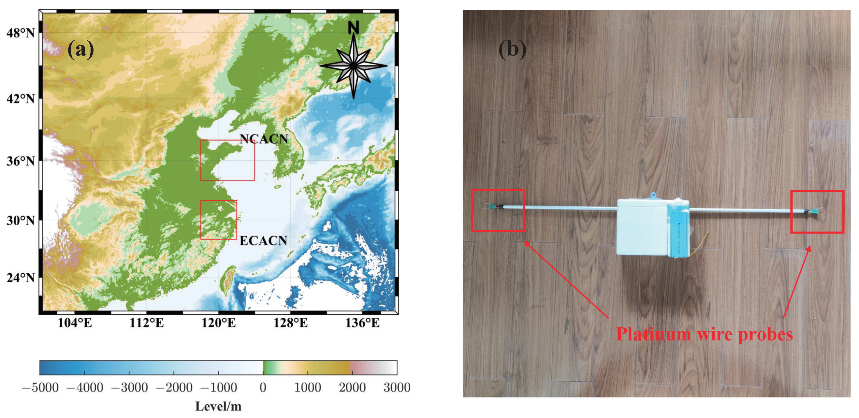
2.1. Experimental Principles
2.2. Scientific Data
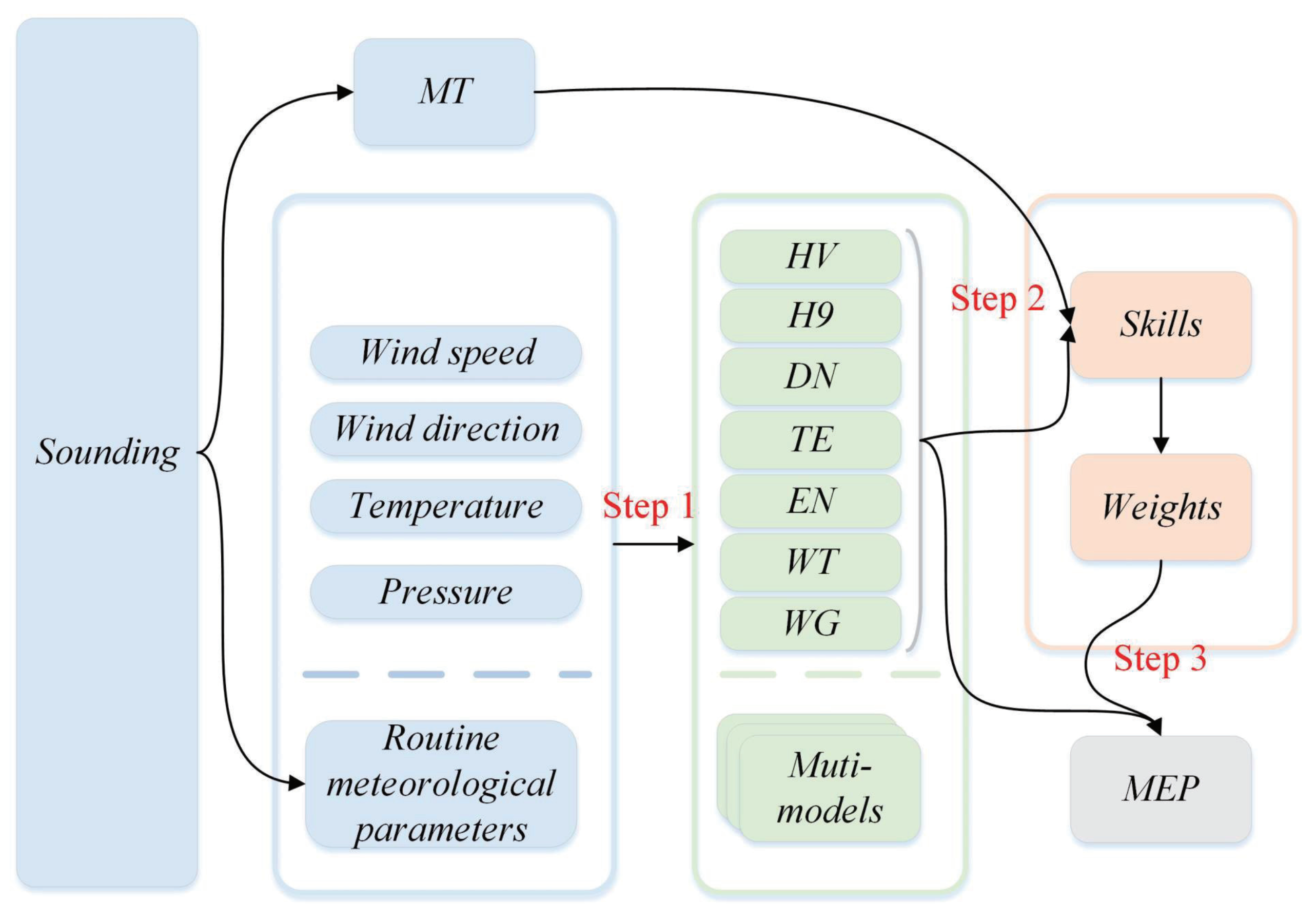
3. Methodology of MEP
3.1. Theory of the Adopted Models
3.2. MEP Method
- 1.
- Using routine meteorological parameters estimating with multiple models;
- 2.
- Obtaining models skills against MT results in Equation (6);
- 3.
- Calculating weights of different models and MEP results.
3.3. Statistical Analysis
4. Results and Discussion
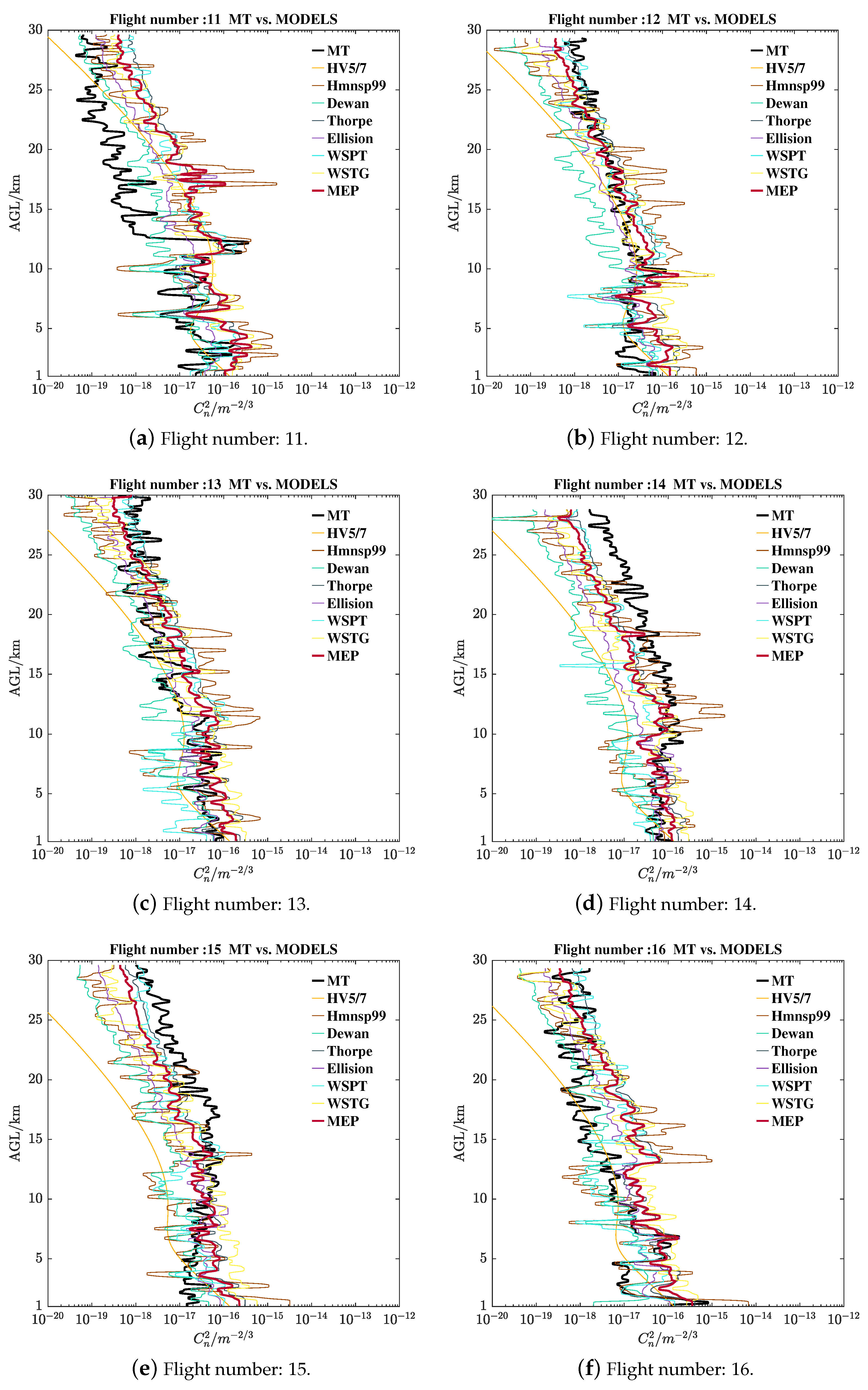
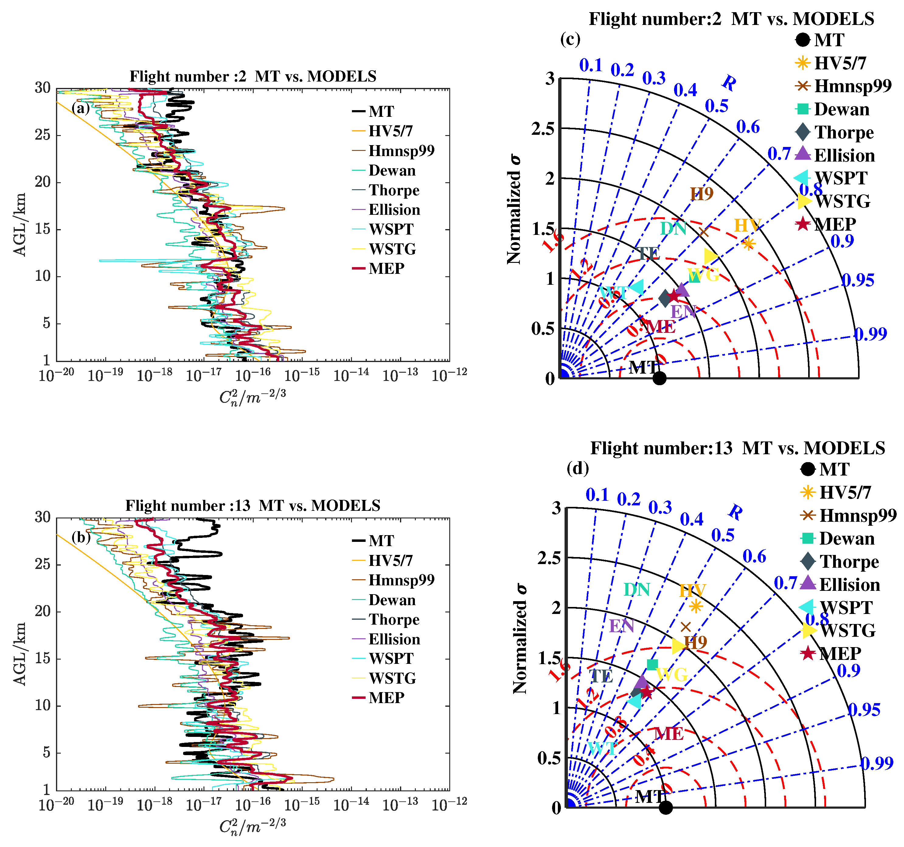
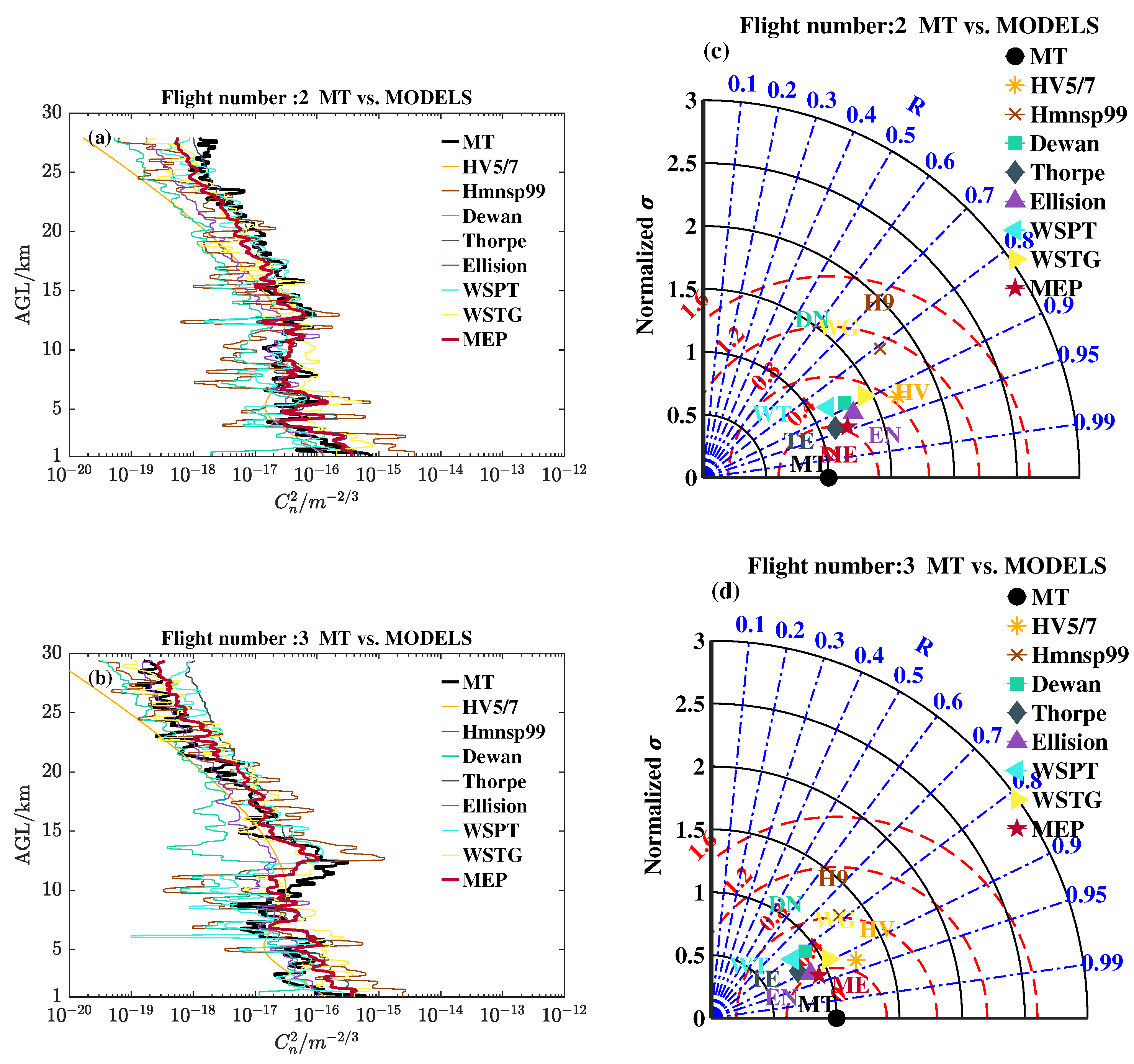
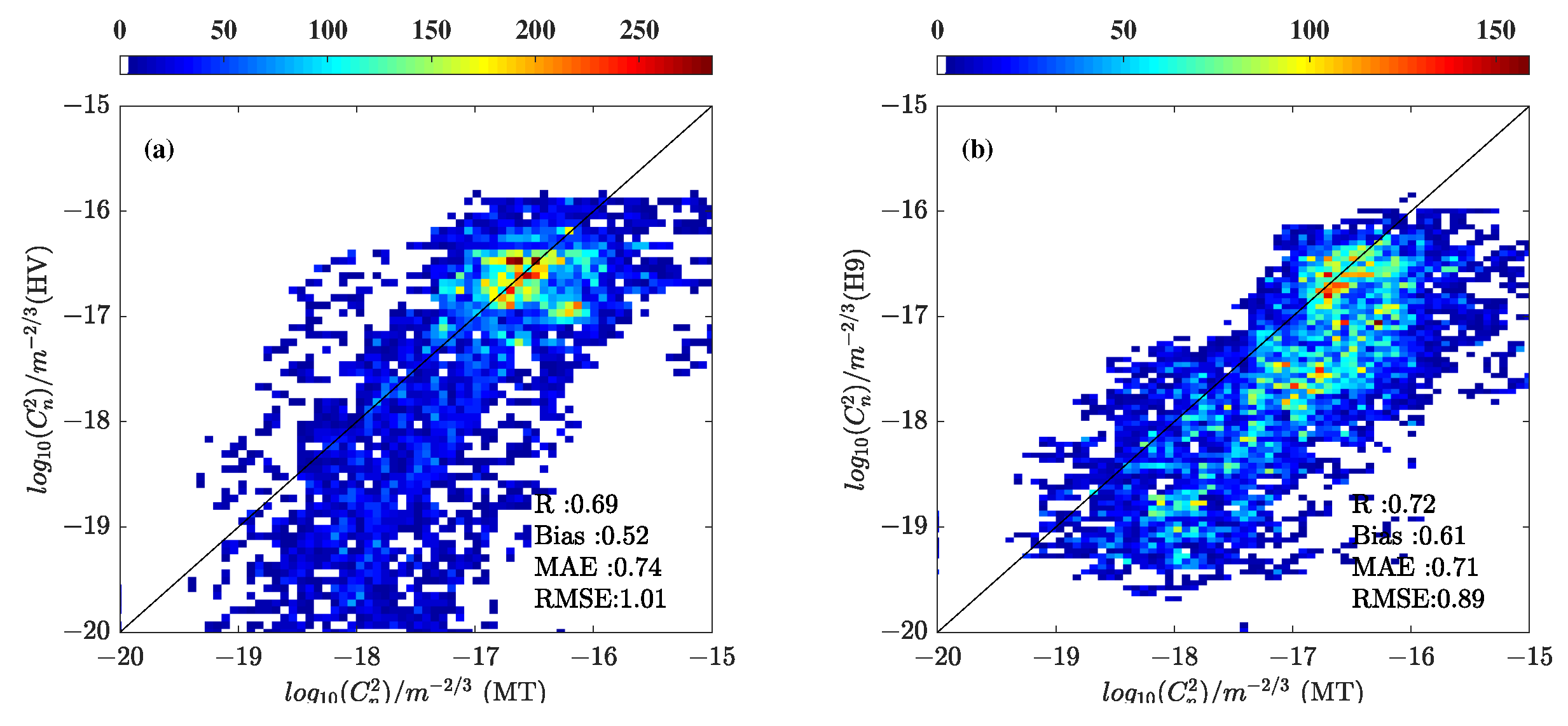
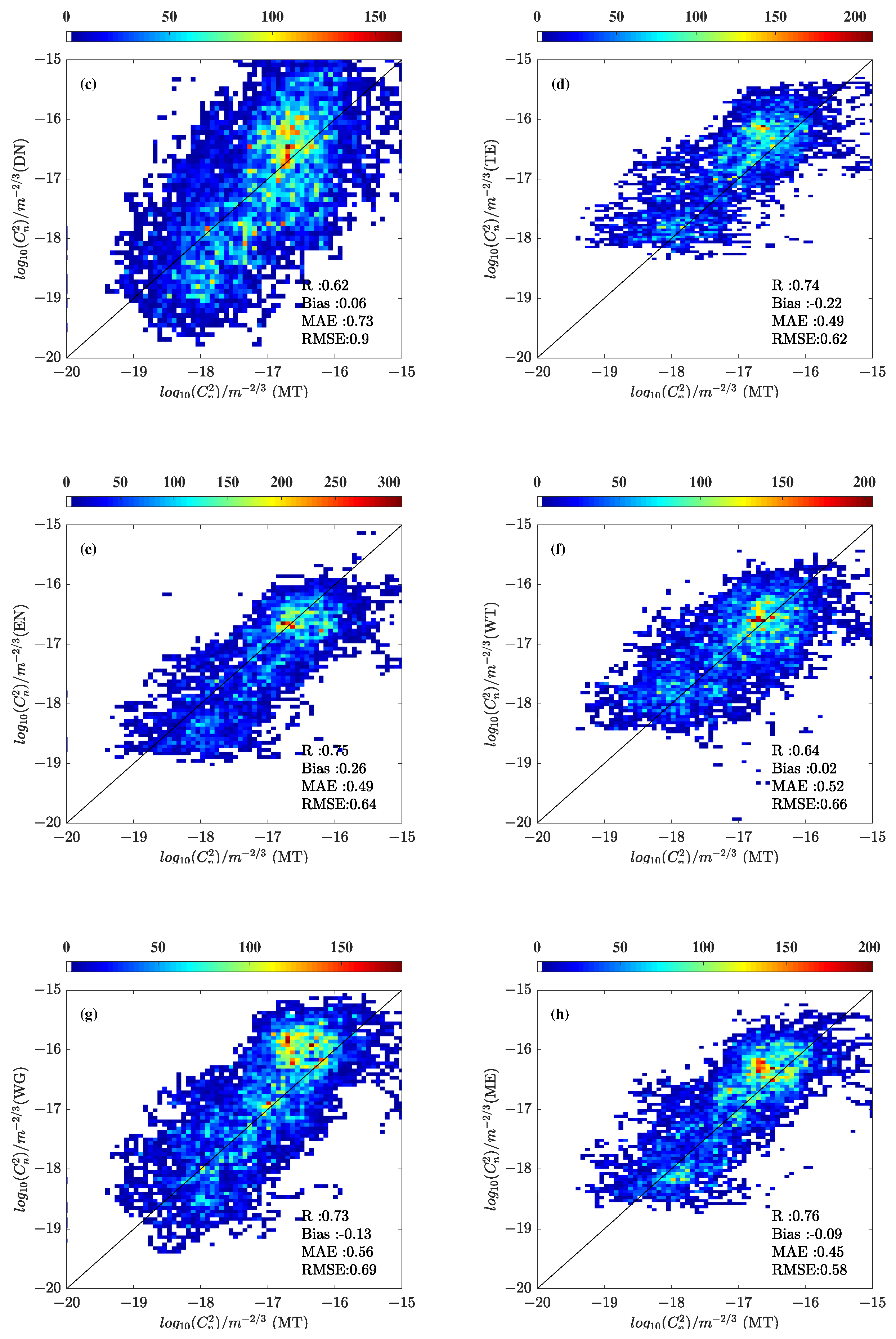
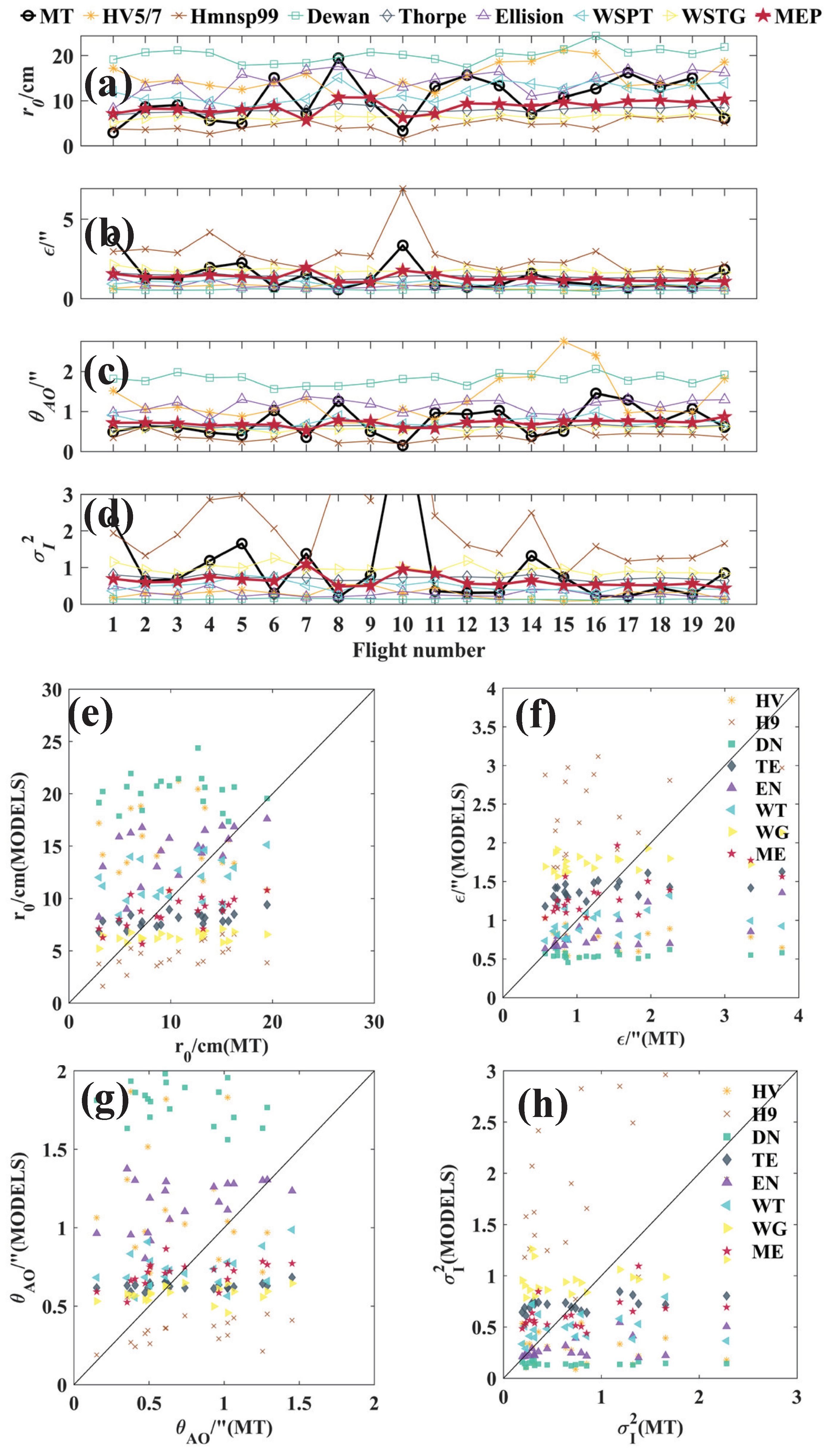
4.1. Measured and Estimated Profiles
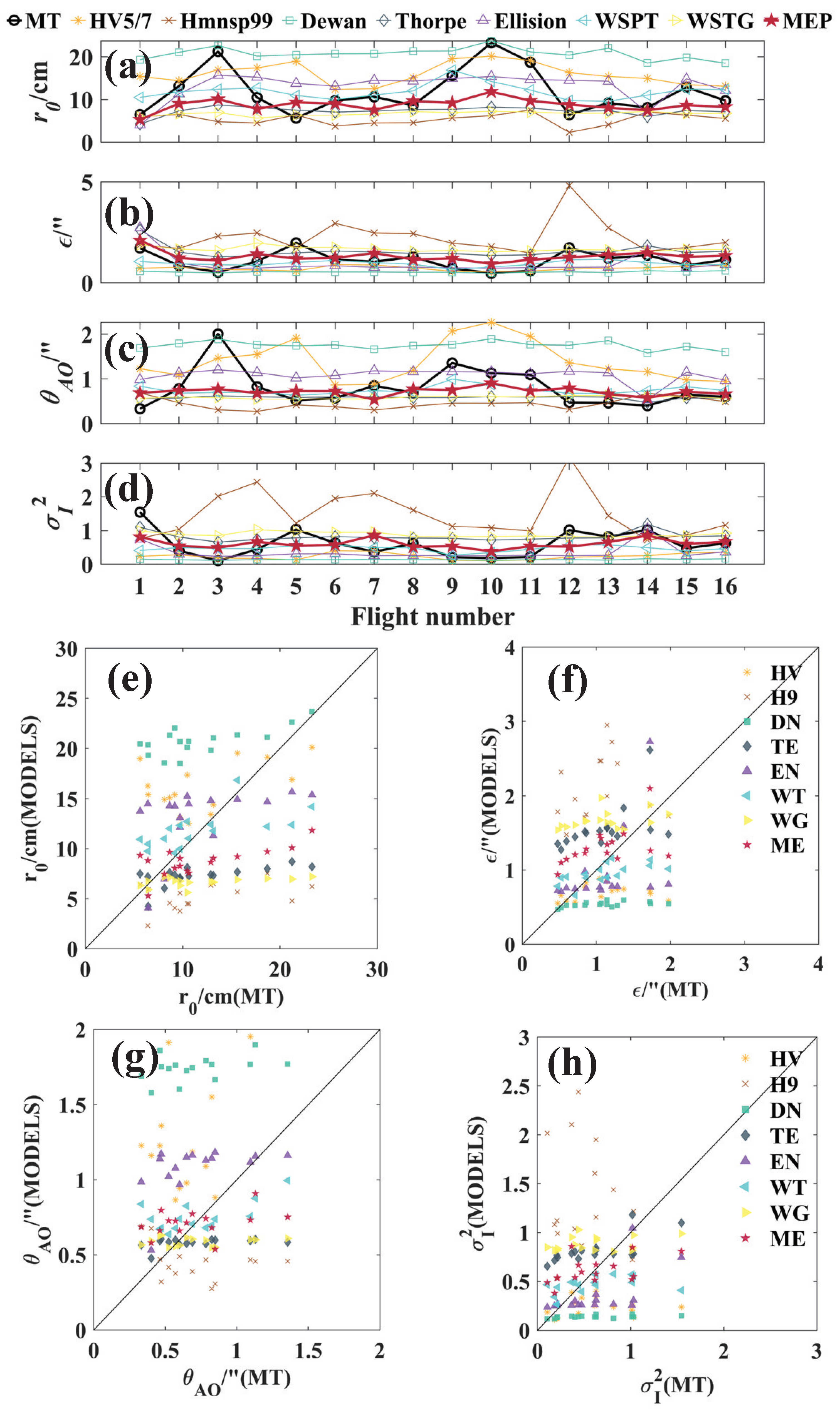
4.2. Integrated Astronomical Parameters from Measured and Estimated Profiles
5. Conclusions
Author Contributions
Funding
Data Availability Statement
Acknowledgments
Conflicts of Interest
Abbreviations
| MEP or ME | Multi-model Ensemble Pattern |
| OT | Optical Turbulence |
| MT | Micro-thermometers |
| SLC | Submarine Laser Communication |
| ECACN | Eastern coastal area of China |
| NCACN | Northern coastal area of China |
| MASS | Multi-Aperture Scintillation Sensor |
| Slodar | Slope Detection And Ranging |
| S-Dimm+ | Solar Differential Image Motion Monitor+ |
| GPS | Global Positioning System |
| AGL | Above the ground level |
| HV5/7 or HV | Hufnagel-Valley5/7 Model |
| H9 | Hmnsp99 Model |
| DN | Dewan Model |
| TE | Thorpe Model |
| EN | Ellison Model |
| WT | WSPT Model |
| WG | WSTG Model |
| AIOFM | Anhui Institute of Optics and Fine Mechanics |
Appendix A. Theories of Adopted Approaches
Appendix A.1. Hufnagel-Valley 5/7 Model
Appendix A.2. The Outer-Scale Method
Appendix A.2.1. Hmnsp99 Model
Appendix A.2.2. Dewan Model
Appendix A.2.3. WSTG Model
Appendix A.3. The Temperature Structure Parameter Method
Appendix A.3.1. Thorpe Model
Appendix A.3.2. Ellison Model
Appendix A.3.3. WSPT Model
Appendix B. Details of Two Areas Radiosonde, Models Estimations, and Integrated Astronomical Parameters Results
Appendix B.1. Radiosonde Details
Appendix B.1.1. ECACN

| Site | Flight Number | Date | Release Time | Flight Duration | Termination Altitude |
|---|---|---|---|---|---|
| (BJT) | /s | (AGL)/m | |||
| 1 | 5 Apirl 2018 | 19:30 | 5010 | 29,020 | |
| 2 | 9 Apirl 2018 | 19:30 | 5027 | 31,210 | |
| 3 | 10 Apirl 2018 | 19:30 | 4767 | 30,410 | |
| 4 | 11 Apirl 2018 | 19:30 | 4788 | 27,880 | |
| 5 | 12 Apirl 2018 | 19:30 | 5014 | 29,810 | |
| 6 | 15 Apirl 2018 | 19:30 | 4088 | 25,740 | |
| 7 | 17 Apirl 2018 | 19:30 | 4355 | 26,410 | |
| 8 | 18 Apirl 2018 | 19:30 | 4686 | 28,150 | |
| ECACN | 9 | 19 Apirl 2018 | 19:30 | 5037 | 30,120 |
| 10 | 20 Apirl 2018 | 19:30 | 5371 | 31,620 | |
| 11 | 22 Apirl 2018 | 19:30 | 4820 | 28,220 | |
| 12 | 24 Apirl 2018 | 19:30 | 5176 | 30,710 | |
| 13 | 25 Apirl 2018 | 19:30 | 5051 | 30,910 | |
| 14 | 26 Apirl 2018 | 19:30 | 5088 | 29,410 | |
| 15 | 27 Apirl 2018 | 19:30 | 5443 | 31,750 | |
| 16 | 28 Apirl 2018 | 19:30 | 5144 | 31,170 |
Appendix B.1.2. NCACN
| Site | Flight Number | Date | Release Time | Flight Duration | Termination Altitude |
|---|---|---|---|---|---|
| (BJT) | /s | (AGL)/m | |||
| 1 | 3 Apirl 2018 | 19:30 | 4464 | 28,660 | |
| 2 | 4 Apirl 2018 | 7:30 | 4210 | 27,970 | |
| 3 | 4 Apirl 2018 | 19:30 | 4747 | 29,460 | |
| 4 | 5 Apirl 2018 | 7:30 | 4808 | 29,320 | |
| 5 | 8 Apirl 2018 | 19:30 | 4271 | 27,370 | |
| 6 | 9 Apirl 2018 | 7:30 | 4855 | 28,880 | |
| 7 | 9 Apirl 2018 | 19:30 | 4780 | 29,660 | |
| 8 | 10 Apirl 2018 | 19:30 | 5275 | 29,780 | |
| 9 | 12 Apirl 2018 | 7:30 | 4591 | 27,810 | |
| 10 | 13 Apirl 2018 | 7:30 | 4633 | 28,710 | |
| NCACN | 11 | 14 Apirl 2018 | 19:30 | 5069 | 29,680 |
| 12 | 16 Apirl 2018 | 7:30 | 5360 | 29,380 | |
| 13 | 16 Apirl 2018 | 19:30 | 5292 | 30,050 | |
| 14 | 17 Apirl 2018 | 7:30 | 5176 | 28,850 | |
| 15 | 20 Apirl 2018 | 7:30 | 5155 | 29,660 | |
| 16 | 21 Apirl 2018 | 19:30 | 4853 | 29,400 | |
| 17 | 25 Apirl 2018 | 19:30 | 5012 | 30,750 | |
| 18 | 26 Apirl 2018 | 7:30 | 4714 | 28,790 | |
| 19 | 26 Apirl 2018 | 19:30 | 4901 | 30,660 | |
| 20 | 27 Apirl 2018 | 19:30 | 4798 | 28,530 |
Appendix B.2. The Refractive Index Structure Parameter of MT and Estimations
Appendix B.2.1. ECACN MT and Models Estimations


Appendix B.2.2. NCACN MT and Models Estimations

Appendix B.3. The Integrated Astronomical Parameters
Appendix B.3.1. ECACN Integrated Astronomical Parameters Details
| Flight | Method | |||||||||
|---|---|---|---|---|---|---|---|---|---|---|
| Parameter | Number | MT | HV | H9 | DN | TE | EN | WT | WG | ME |
| 1 | 6.45 | 15.41 | 5.95 | 19.31 | 4.25 | 4.08 | 10.48 | 5.92 | 5.30 | |
| 2 | 13.15 | 14.38 | 6.52 | 21.05 | 7.33 | 11.32 | 11.79 | 6.67 | 9.05 | |
| 3 | 21.22 | 16.91 | 4.80 | 22.64 | 8.72 | 15.68 | 12.40 | 6.98 | 10.10 | |
| 4 | 10.47 | 17.37 | 4.51 | 20.13 | 8.13 | 15.24 | 12.73 | 5.64 | 7.78 | |
| 5 | 5.63 | 18.97 | 6.43 | 20.46 | 7.50 | 13.76 | 10.94 | 6.34 | 9.34 | |
| 6 | 9.72 | 12.37 | 3.77 | 20.69 | 7.05 | 13.10 | 9.98 | 6.33 | 9.03 | |
| 7 | 10.63 | 12.53 | 4.51 | 20.72 | 7.28 | 14.47 | 11.04 | 6.64 | 7.56 | |
| 8 | 8.66 | 15.11 | 4.57 | 21.32 | 7.64 | 14.30 | 12.02 | 7.14 | 9.65 | |
| 9 | 15.61 | 19.53 | 5.68 | 21.35 | 7.69 | 14.93 | 16.86 | 6.92 | 9.21 | |
| /cm | 10 | 23.28 | 20.11 | 6.23 | 23.69 | 8.21 | 15.39 | 14.21 | 7.22 | 11.84 |
| 11 | 18.69 | 19.12 | 7.52 | 21.14 | 8.01 | 14.69 | 12.23 | 7.03 | 9.71 | |
| 12 | 6.43 | 16.28 | 2.31 | 20.37 | 7.21 | 14.47 | 9.76 | 6.78 | 8.82 | |
| 13 | 9.19 | 15.40 | 4.08 | 22.02 | 7.38 | 14.27 | 9.58 | 6.82 | 8.06 | |
| 14 | 8.12 | 14.94 | 7.06 | 18.54 | 6.05 | 6.97 | 11.01 | 7.19 | 7.47 | |
| 15 | 12.90 | 13.44 | 6.36 | 19.82 | 7.41 | 14.82 | 12.43 | 6.70 | 8.66 | |
| 16 | 9.72 | 13.12 | 5.57 | 18.49 | 7.11 | 12.14 | 12.34 | 6.78 | 8.27 | |
| Median | 10.10 | 15.41 | 5.63 | 20.70 | 7.39 | 14.38 | 11.91 | 6.78 | 8.93 | |
| Mean | 11.87 | 15.94 | 5.37 | 20.73 | 7.31 | 13.10 | 11.86 | 6.69 | 8.74 |
| Flight | Method | |||||||||
|---|---|---|---|---|---|---|---|---|---|---|
| Parameter | Number | MT | HV | H9 | DN | TE | EN | WT | WG | ME |
| 1 | 1.72 | 0.72 | 1.87 | 0.58 | 2.61 | 2.73 | 1.06 | 1.88 | 2.10 | |
| 2 | 0.85 | 0.77 | 1.71 | 0.53 | 1.52 | 0.98 | 0.94 | 1.67 | 1.23 | |
| 3 | 0.52 | 0.66 | 2.32 | 0.49 | 1.28 | 0.71 | 0.90 | 1.59 | 1.10 | |
| 4 | 1.06 | 0.64 | 2.47 | 0.55 | 1.37 | 0.73 | 0.87 | 1.97 | 1.43 | |
| 5 | 1.97 | 0.59 | 1.73 | 0.54 | 1.48 | 0.81 | 1.02 | 1.75 | 1.19 | |
| 6 | 1.14 | 0.90 | 2.95 | 0.54 | 1.58 | 0.85 | 1.11 | 1.76 | 1.23 | |
| 7 | 1.05 | 0.89 | 2.47 | 0.54 | 1.53 | 0.77 | 1.01 | 1.67 | 1.47 | |
| 8 | 1.28 | 0.74 | 2.43 | 0.52 | 1.46 | 0.78 | 0.92 | 1.56 | 1.15 | |
| 9 | 0.71 | 0.57 | 1.96 | 0.52 | 1.45 | 0.74 | 0.66 | 1.61 | 1.21 | |
| / | 10 | 0.48 | 0.55 | 1.79 | 0.47 | 1.35 | 0.72 | 0.78 | 1.54 | 0.94 |
| 11 | 0.59 | 0.58 | 1.48 | 0.53 | 1.39 | 0.76 | 0.91 | 1.58 | 1.15 | |
| 12 | 1.73 | 0.68 | 4.81 | 0.55 | 1.54 | 0.77 | 1.14 | 1.64 | 1.26 | |
| 13 | 1.21 | 0.72 | 2.72 | 0.50 | 1.51 | 0.78 | 1.16 | 1.63 | 1.38 | |
| 14 | 1.37 | 0.74 | 1.57 | 0.60 | 1.84 | 1.59 | 1.01 | 1.55 | 1.49 | |
| 15 | 0.86 | 0.83 | 1.75 | 0.56 | 1.50 | 0.75 | 0.89 | 1.66 | 1.28 | |
| 16 | 1.14 | 0.85 | 1.99 | 0.60 | 1.56 | 0.92 | 0.90 | 1.64 | 1.34 | |
| Median | 1.10 | 0.72 | 1.98 | 0.54 | 1.50 | 0.77 | 0.93 | 1.64 | 1.25 | |
| Mean | 1.11 | 0.71 | 2.25 | 0.54 | 1.56 | 0.96 | 0.96 | 1.67 | 1.31 |
| Flight | Method | |||||||||
|---|---|---|---|---|---|---|---|---|---|---|
| Parameter | Number | MT | HV | H9 | DN | TE | EN | WT | WG | ME |
| 1 | 0.33 | 1.23 | 0.69 | 1.69 | 0.57 | 0.99 | 0.84 | 0.57 | 0.69 | |
| 2 | 0.78 | 1.09 | 0.47 | 1.79 | 0.57 | 1.13 | 0.68 | 0.60 | 0.74 | |
| 3 | 2.01 | 1.47 | 0.31 | 1.89 | 0.62 | 1.20 | 0.70 | 0.58 | 0.77 | |
| 4 | 0.83 | 1.55 | 0.28 | 1.77 | 0.60 | 1.14 | 0.70 | 0.55 | 0.68 | |
| 5 | 0.52 | 1.91 | 0.42 | 1.74 | 0.59 | 1.02 | 0.64 | 0.55 | 0.73 | |
| 6 | 0.57 | 0.87 | 0.38 | 1.76 | 0.60 | 1.08 | 0.68 | 0.56 | 0.73 | |
| 7 | 0.85 | 0.88 | 0.31 | 1.67 | 0.60 | 1.18 | 0.74 | 0.55 | 0.54 | |
| 8 | 0.69 | 1.18 | 0.39 | 1.75 | 0.58 | 1.16 | 0.71 | 0.61 | 0.77 | |
| 9 | 1.36 | 2.07 | 0.46 | 1.77 | 0.58 | 1.16 | 1.00 | 0.61 | 0.75 | |
| / | 10 | 1.13 | 2.27 | 0.46 | 1.90 | 0.60 | 1.16 | 0.88 | 0.60 | 0.91 |
| 11 | 1.10 | 1.95 | 0.47 | 1.77 | 0.59 | 1.12 | 0.76 | 0.60 | 0.73 | |
| 12 | 0.47 | 1.36 | 0.32 | 1.75 | 0.61 | 1.17 | 0.68 | 0.63 | 0.80 | |
| 13 | 0.46 | 1.23 | 0.47 | 1.86 | 0.59 | 1.14 | 0.67 | 0.63 | 0.66 | |
| 14 | 0.40 | 1.16 | 0.68 | 1.58 | 0.48 | 0.53 | 0.74 | 0.59 | 0.58 | |
| 15 | 0.65 | 0.98 | 0.61 | 1.73 | 0.58 | 1.15 | 0.83 | 0.62 | 0.71 | |
| 16 | 0.60 | 0.94 | 0.49 | 1.60 | 0.57 | 0.97 | 0.74 | 0.56 | 0.66 | |
| Median | 0.67 | 1.23 | 0.46 | 1.76 | 0.59 | 1.14 | 0.72 | 0.60 | 0.73 | |
| Mean | 0.80 | 1.38 | 0.45 | 1.75 | 0.58 | 1.08 | 0.75 | 0.59 | 0.72 |
| Flight | Method | |||||||||
|---|---|---|---|---|---|---|---|---|---|---|
| Parameter | Number | MT | HV | H9 | DN | TE | EN | WT | WG | ME |
| 1 | 1.54 | 0.24 | 0.76 | 0.15 | 1.10 | 0.75 | 0.41 | 0.99 | 0.81 | |
| 2 | 0.40 | 0.28 | 1.04 | 0.13 | 0.80 | 0.30 | 0.49 | 0.87 | 0.54 | |
| 3 | 0.10 | 0.19 | 2.02 | 0.12 | 0.66 | 0.24 | 0.47 | 0.85 | 0.49 | |
| 4 | 0.44 | 0.17 | 2.44 | 0.14 | 0.73 | 0.26 | 0.46 | 1.03 | 0.67 | |
| 5 | 1.03 | 0.13 | 1.22 | 0.14 | 0.78 | 0.31 | 0.56 | 0.97 | 0.55 | |
| 6 | 0.63 | 0.40 | 1.95 | 0.14 | 0.82 | 0.31 | 0.57 | 0.95 | 0.58 | |
| 7 | 0.37 | 0.39 | 2.10 | 0.14 | 0.79 | 0.26 | 0.49 | 0.95 | 0.86 | |
| 8 | 0.61 | 0.25 | 1.61 | 0.14 | 0.78 | 0.26 | 0.49 | 0.82 | 0.51 | |
| 9 | 0.21 | 0.12 | 1.12 | 0.13 | 0.77 | 0.26 | 0.27 | 0.82 | 0.54 | |
| 10 | 0.18 | 0.11 | 1.08 | 0.12 | 0.72 | 0.25 | 0.34 | 0.82 | 0.38 | |
| 11 | 0.22 | 0.13 | 0.99 | 0.14 | 0.75 | 0.27 | 0.44 | 0.84 | 0.54 | |
| 12 | 1.01 | 0.21 | 3.18 | 0.14 | 0.78 | 0.26 | 0.57 | 0.82 | 0.52 | |
| 13 | 0.82 | 0.24 | 1.44 | 0.12 | 0.78 | 0.27 | 0.58 | 0.81 | 0.66 | |
| 14 | 1.02 | 0.26 | 0.72 | 0.17 | 1.18 | 1.05 | 0.49 | 0.84 | 0.85 | |
| 15 | 0.47 | 0.33 | 0.87 | 0.14 | 0.82 | 0.26 | 0.40 | 0.84 | 0.60 | |
| 16 | 0.63 | 0.35 | 1.16 | 0.16 | 0.84 | 0.37 | 0.46 | 0.92 | 0.67 | |
| Median | 0.54 | 0.24 | 1.19 | 0.14 | 0.78 | 0.26 | 0.48 | 0.85 | 0.56 | |
| Mean | 0.61 | 0.24 | 1.48 | 0.14 | 0.82 | 0.35 | 0.47 | 0.88 | 0.61 |
Appendix B.3.2. NCACN Integrated Astronomical Parameters Details
| Flight | Method | |||||||||
|---|---|---|---|---|---|---|---|---|---|---|
| Parameter | Number | MT | HV | H9 | DN | TE | EN | WT | WG | ME |
| 1 | 2.95 | 17.18 | 3.74 | 19.16 | 6.84 | 8.21 | 12.00 | 5.21 | 7.12 | |
| 2 | 8.63 | 14.05 | 3.57 | 20.75 | 7.36 | 13.01 | 10.20 | 6.15 | 8.27 | |
| 3 | 9.04 | 14.56 | 3.85 | 21.19 | 7.50 | 14.53 | 10.75 | 6.64 | 8.16 | |
| 4 | 5.67 | 13.40 | 2.67 | 20.68 | 6.90 | 8.99 | 9.81 | 5.77 | 7.40 | |
| 5 | 4.93 | 12.47 | 3.96 | 17.86 | 7.79 | 15.88 | 8.42 | 6.19 | 8.03 | |
| 6 | 15.11 | 13.97 | 4.86 | 18.12 | 7.82 | 14.03 | 9.47 | 5.81 | 8.84 | |
| 7 | 7.19 | 15.95 | 5.82 | 18.41 | 7.76 | 16.78 | 10.38 | 6.20 | 5.66 | |
| 8 | 19.46 | 10.79 | 3.86 | 19.55 | 9.41 | 17.60 | 15.12 | 6.57 | 10.77 | |
| 9 | 9.86 | 10.72 | 4.16 | 20.76 | 8.94 | 15.73 | 10.18 | 6.40 | 10.73 | |
| 10 | 3.32 | 14.17 | 1.61 | 20.21 | 7.85 | 13.02 | 11.18 | 6.46 | 6.27 | |
| 11 | 13.17 | 11.67 | 3.99 | 19.27 | 7.60 | 14.78 | 9.66 | 6.57 | 7.11 | |
| 12 | 15.67 | 15.55 | 5.16 | 17.36 | 7.84 | 15.65 | 12.09 | 5.93 | 9.40 | |
| 13 | 13.35 | 18.65 | 6.17 | 20.62 | 8.16 | 16.50 | 14.61 | 6.91 | 9.29 | |
| 14 | 7.06 | 18.80 | 4.77 | 20.02 | 7.42 | 11.02 | 13.74 | 6.24 | 8.79 | |
| 15 | 10.77 | 21.23 | 4.92 | 21.43 | 8.19 | 12.19 | 12.68 | 6.11 | 9.73 | |
| 16 | 12.67 | 20.45 | 3.74 | 24.38 | 8.56 | 14.97 | 14.64 | 6.84 | 8.83 | |
| 17 | 16.23 | 13.34 | 6.61 | 20.65 | 8.50 | 16.84 | 12.93 | 6.82 | 9.93 | |
| 18 | 13.03 | 13.83 | 6.00 | 21.46 | 8.35 | 14.32 | 12.10 | 6.31 | 10.11 | |
| 19 | 15.06 | 13.40 | 6.60 | 20.38 | 8.86 | 16.90 | 13.65 | 7.10 | 9.62 | |
| 20 | 6.06 | 18.60 | 5.22 | 21.95 | 8.43 | 16.24 | 13.98 | 6.75 | 10.36 | |
| Median | 10.31 | 14.11 | 4.46 | 20.50 | 7.84 | 14.88 | 12.04 | 6.36 | 8.83 | |
| Mean | 10.46 | 15.14 | 4.56 | 20.21 | 8.00 | 14.36 | 11.88 | 6.35 | 8.72 |
| Flight | Method | |||||||||
|---|---|---|---|---|---|---|---|---|---|---|
| Parameter | Number | MT | HV | H9 | DN | TE | EN | WT | WG | ME |
| 1 | 3.77 | 0.65 | 2.97 | 0.58 | 1.63 | 1.35 | 0.93 | 2.13 | 1.56 | |
| 2 | 1.29 | 0.79 | 3.12 | 0.54 | 1.51 | 0.85 | 1.09 | 1.81 | 1.34 | |
| 3 | 1.23 | 0.76 | 2.88 | 0.52 | 1.48 | 0.76 | 1.03 | 1.67 | 1.36 | |
| 4 | 1.96 | 0.83 | 4.17 | 0.54 | 1.61 | 1.24 | 1.13 | 1.93 | 1.50 | |
| 5 | 2.26 | 0.89 | 2.81 | 0.62 | 1.43 | 0.70 | 1.32 | 1.80 | 1.39 | |
| 6 | 0.74 | 0.80 | 2.29 | 0.61 | 1.42 | 0.79 | 1.17 | 1.91 | 1.26 | |
| 7 | 1.55 | 0.70 | 1.91 | 0.60 | 1.43 | 0.66 | 1.07 | 1.79 | 1.97 | |
| 8 | 0.57 | 1.03 | 2.88 | 0.57 | 1.18 | 0.63 | 0.74 | 1.69 | 1.03 | |
| 9 | 1.13 | 1.04 | 2.67 | 0.54 | 1.24 | 0.71 | 1.09 | 1.74 | 1.04 | |
| / | 10 | 3.35 | 0.78 | 6.92 | 0.55 | 1.42 | 0.85 | 0.99 | 1.72 | 1.77 |
| 11 | 0.84 | 0.95 | 2.79 | 0.58 | 1.46 | 0.75 | 1.15 | 1.69 | 1.56 | |
| 12 | 0.71 | 0.71 | 2.16 | 0.64 | 1.42 | 0.71 | 0.92 | 1.87 | 1.18 | |
| 13 | 0.83 | 0.60 | 1.80 | 0.54 | 1.36 | 0.67 | 0.76 | 1.61 | 1.20 | |
| 14 | 1.57 | 0.59 | 2.33 | 0.56 | 1.50 | 1.01 | 0.81 | 1.78 | 1.26 | |
| 15 | 1.03 | 0.52 | 2.26 | 0.52 | 1.36 | 0.91 | 0.88 | 1.82 | 1.14 | |
| 16 | 0.88 | 0.54 | 2.97 | 0.46 | 1.30 | 0.74 | 0.76 | 1.62 | 1.26 | |
| 17 | 0.69 | 0.83 | 1.68 | 0.54 | 1.31 | 0.66 | 0.86 | 1.63 | 1.12 | |
| 18 | 0.85 | 0.80 | 1.85 | 0.52 | 1.33 | 0.78 | 0.92 | 1.76 | 1.10 | |
| 19 | 0.74 | 0.83 | 1.68 | 0.55 | 1.25 | 0.66 | 0.81 | 1.57 | 1.16 | |
| 20 | 1.83 | 0.60 | 2.13 | 0.51 | 1.32 | 0.68 | 0.80 | 1.65 | 1.07 | |
| Median | 1.08 | 0.79 | 2.50 | 0.54 | 1.42 | 0.75 | 0.92 | 1.75 | 1.26 | |
| Mean | 1.39 | 0.76 | 2.71 | 0.55 | 1.40 | 0.81 | 0.96 | 1.76 | 1.31 |
| Flight | Method | |||||||||
|---|---|---|---|---|---|---|---|---|---|---|
| Parameter | Number | MT | HV | H9 | DN | TE | EN | WT | WG | ME |
| 1 | 0.49 | 1.52 | 0.35 | 1.82 | 0.62 | 0.97 | 0.91 | 0.54 | 0.72 | |
| 2 | 0.64 | 1.05 | 0.62 | 1.76 | 0.63 | 1.05 | 0.73 | 0.59 | 0.72 | |
| 3 | 0.61 | 1.11 | 0.36 | 1.98 | 0.66 | 1.23 | 0.69 | 0.63 | 0.71 | |
| 4 | 0.47 | 0.97 | 0.33 | 1.84 | 0.59 | 0.80 | 0.68 | 0.54 | 0.65 | |
| 5 | 0.41 | 0.88 | 0.24 | 1.86 | 0.63 | 1.30 | 0.55 | 0.57 | 0.67 | |
| 6 | 1.02 | 1.04 | 0.31 | 1.56 | 0.62 | 1.11 | 0.56 | 0.46 | 0.67 | |
| 7 | 0.35 | 1.31 | 0.56 | 1.63 | 0.63 | 1.38 | 0.68 | 0.58 | 0.53 | |
| 8 | 1.26 | 0.72 | 0.21 | 1.63 | 0.64 | 1.30 | 0.88 | 0.56 | 0.78 | |
| 9 | 0.51 | 0.71 | 0.26 | 1.71 | 0.65 | 1.19 | 0.63 | 0.57 | 0.75 | |
| / | 10 | 0.15 | 1.06 | 0.19 | 1.81 | 0.62 | 0.96 | 0.68 | 0.53 | 0.59 |
| 11 | 0.97 | 0.80 | 0.29 | 1.86 | 0.64 | 1.16 | 0.65 | 0.61 | 0.59 | |
| 12 | 0.93 | 1.25 | 0.37 | 1.65 | 0.61 | 1.26 | 0.74 | 0.50 | 0.73 | |
| 13 | 1.02 | 1.83 | 0.39 | 1.96 | 0.61 | 1.28 | 0.78 | 0.65 | 0.77 | |
| 14 | 0.38 | 1.87 | 0.27 | 1.93 | 0.59 | 0.95 | 0.83 | 0.57 | 0.66 | |
| 15 | 0.51 | 2.75 | 0.75 | 1.80 | 0.63 | 0.92 | 0.79 | 0.58 | 0.76 | |
| 16 | 1.45 | 2.40 | 0.41 | 2.06 | 0.68 | 1.23 | 0.99 | 0.65 | 0.77 | |
| 17 | 1.29 | 0.97 | 0.45 | 1.77 | 0.63 | 1.31 | 0.66 | 0.59 | 0.77 | |
| 18 | 0.74 | 1.02 | 0.44 | 1.89 | 0.62 | 1.10 | 0.71 | 0.65 | 0.75 | |
| 19 | 1.06 | 0.97 | 0.43 | 1.70 | 0.62 | 1.28 | 0.77 | 0.59 | 0.73 | |
| 20 | 0.61 | 1.82 | 0.36 | 1.93 | 0.66 | 1.29 | 0.74 | 0.63 | 0.87 | |
| Median | 0.63 | 1.06 | 0.36 | 1.82 | 0.63 | 1.21 | 0.72 | 0.58 | 0.72 | |
| Mean | 0.74 | 1.30 | 0.38 | 1.81 | 0.63 | 1.15 | 0.73 | 0.58 | 0.71 |
| Flight | Method | |||||||||
|---|---|---|---|---|---|---|---|---|---|---|
| Parameter | Number | MT | HV | H9 | DN | TE | EN | WT | WG | ME |
| 1 | 2.28 | 0.18 | 1.94 | 0.14 | 0.80 | 0.50 | 0.36 | 1.16 | 0.69 | |
| 2 | 0.63 | 0.30 | 1.33 | 0.14 | 0.74 | 0.32 | 0.50 | 0.94 | 0.60 | |
| 3 | 0.69 | 0.27 | 1.90 | 0.12 | 0.69 | 0.25 | 0.52 | 0.82 | 0.62 | |
| 4 | 1.19 | 0.33 | 2.85 | 0.14 | 0.85 | 0.54 | 0.58 | 1.06 | 0.74 | |
| 5 | 1.66 | 0.39 | 2.96 | 0.15 | 0.72 | 0.22 | 0.79 | 0.99 | 0.68 | |
| 6 | 0.29 | 0.30 | 2.07 | 0.17 | 0.73 | 0.29 | 0.72 | 1.26 | 0.64 | |
| 7 | 1.38 | 0.22 | 0.99 | 0.16 | 0.73 | 0.20 | 0.53 | 0.97 | 1.10 | |
| 8 | 0.19 | 0.53 | 3.69 | 0.16 | 0.64 | 0.21 | 0.33 | 0.96 | 0.49 | |
| 9 | 0.79 | 0.54 | 2.83 | 0.14 | 0.65 | 0.25 | 0.63 | 0.93 | 0.50 | |
| 10 | 5.37 | 0.29 | 8.17 | 0.14 | 0.73 | 0.35 | 0.52 | 1.01 | 0.96 | |
| 11 | 0.36 | 0.45 | 2.42 | 0.14 | 0.74 | 0.26 | 0.62 | 0.88 | 0.85 | |
| 12 | 0.31 | 0.23 | 1.62 | 0.17 | 0.75 | 0.23 | 0.47 | 1.19 | 0.56 | |
| 13 | 0.32 | 0.14 | 1.40 | 0.13 | 0.72 | 0.22 | 0.40 | 0.80 | 0.54 | |
| 14 | 1.32 | 0.14 | 2.49 | 0.13 | 0.81 | 0.41 | 0.38 | 0.99 | 0.65 | |
| 15 | 0.74 | 0.09 | 0.77 | 0.13 | 0.68 | 0.39 | 0.41 | 0.96 | 0.51 | |
| 16 | 0.23 | 0.10 | 1.58 | 0.11 | 0.61 | 0.24 | 0.29 | 0.79 | 0.54 | |
| 17 | 0.22 | 0.34 | 1.18 | 0.14 | 0.69 | 0.21 | 0.51 | 0.91 | 0.52 | |
| 18 | 0.45 | 0.31 | 1.25 | 0.13 | 0.72 | 0.29 | 0.48 | 0.86 | 0.52 | |
| 19 | 0.27 | 0.33 | 1.26 | 0.15 | 0.69 | 0.22 | 0.41 | 0.86 | 0.57 | |
| 20 | 0.85 | 0.14 | 1.66 | 0.12 | 0.64 | 0.22 | 0.41 | 0.84 | 0.44 | |
| Median | 0.66 | 0.30 | 1.78 | 0.14 | 0.72 | 0.25 | 0.49 | 0.95 | 0.58 | |
| Mean | 0.98 | 0.28 | 2.22 | 0.14 | 0.72 | 0.29 | 0.49 | 0.96 | 0.64 |
References
- Tatarskii, V.I. Wave Propagation in a Turbulent Medium; McGraw-Hill: New York, NY, USA, 1961. [Google Scholar]
- Beckers, J.M. Adaptive optics for astronomy: Principles, performance, and applications. Annu. Rev. Astron. Astrophys. 1993, 31, 13–62. [Google Scholar] [CrossRef]
- Coulman, C.E. Fundmental and applied aspects of astronomical seeing. Annu. Rev. Astron. Astrophys. 1985, 23, 19–57. [Google Scholar] [CrossRef]
- Davies, R.; Kasper, M. Adaptive Optics for Astronomy. Annu. Rev. Astron. Astrophys. 2012, 50, 305–351. [Google Scholar] [CrossRef] [Green Version]
- Fried, D.L. Limiting resolution looking down through the atmosphere. J. Opt. Soc. Am. 1966, 56, 1380–1385. [Google Scholar] [CrossRef]
- Deng, L.; Yang, F.; Chen, X.; He, F.; Liu, Q.; Zhang, B.; Zhang, C.; Wang, K.; Liu, N.; Ren, A.; et al. Lenghu on the Tibetan Plateau as an astronomical observing site. Nature 2021, 596, 353. [Google Scholar] [CrossRef] [PubMed]
- Fugate, R.Q.; Fried, D.L.; Ameer, G.A.; Boeke, B.R.; Browne, S.L.; Roberts, P.H.; Ruane, R.E.; Tyler, G.A.; Wopat, L.M. Measurement of atmospheric wave-front distortion using scatterd-light from a laser guide-star. Nature 1991, 353, 144–146. [Google Scholar] [CrossRef]
- Mahalov, A.; Moustaoui, M. Characterization of atmospheric optical turbulence for laser propagation. Laser Photonics Rev. 2010, 4, 144–159. [Google Scholar] [CrossRef]
- Roddier, F. V the Effects of Atmospheric Turbulence in Optical Astronomy. In Progress in Optics; Wolf, E., Ed.; Elsevier: Amsterdam, The Netherlands, 1981; Volume 19, pp. 281–376. [Google Scholar] [CrossRef]
- Zhang, R.Z.; Hu, N.Z.; Zhou, H.B.; Zou, K.H.; Su, X.Z.; Zhou, Y.Y.; Song, H.Q.; Pang, K.; Song, H.; Minoofar, A.; et al. Turbulence-resilient pilot-assisted self-coherent free-space optical communications using automatic optoelectronic mixing of many modes. Nat. Photonics 2021, 15, 743–750. [Google Scholar] [CrossRef]
- Zhu, Z.; Janasik, M.; Fyffe, A.; Hay, D.; Zhou, Y.; Kantor, B.; Winder, T.; Boyd, R.W.; Leuchs, G.; Shi, Z. Compensation-free high-dimensional free-space optical communication using turbulence-resilient vector beams. Nat. Commun. 2021, 12, 1666. [Google Scholar] [CrossRef]
- Masciadri, E.; Vernin, J.; Bougeault, P. 3D mapping of optical turbulence using an atmospheric numerical model I. A useful tool for the ground-based astronomy. Astron. Astrophys. Suppl. Ser. 1999, 137, 185–202. [Google Scholar] [CrossRef] [Green Version]
- Marks, R.D.; Vernin, J.; Azouit, M.; Briggs, J.W.; Burton, M.G.; Ashley, M.C.B.; Manigault, J.F. Antarctic site testing–Microthermal measurements of surface-layer seeing at the South Pole. Astron. Astrophys. Suppl. Ser. 1996, 118, 385–390. [Google Scholar] [CrossRef]
- Qing, C.; Wu, X.; Li, X.; Luo, T.; Su, C.; Zhu, W. Mesoscale optical turbulence simulations above Tibetan Plateau: First attempt. Opt. Express 2020, 28, 4571–4586. [Google Scholar] [CrossRef] [PubMed]
- Guryanov, A.E.; Kallistratova, M.A.; Kutyrev, A.S.; Petenko, I.V.; Shcheglov, P.V.; Tokovinin, A.A. The contribution of the lower atmospheric layers to the seeing at some mountain observatories. Astron. Astrophys. 1992, 262, 373–381. [Google Scholar]
- Tokovinin, A.; Kornilov, V. Measuring turbulence profile from scintillations of single stars. In Astronomical Site Evaluation in the Visible and Radio Range Workshop, IAU Technical Workshop, Proceedings of a Workshop Held at Cadi Ayyad University, Marrakech, Morocco, 13–17 November 2000; Astronomical Society of the Pacific Conference Series; Astronomical Soc Pacific: San Francisco, CA, USA, 2002; Volume 266, pp. 104–112. [Google Scholar]
- Osborn, J.; Wilson, R.; Butterley, T.; Shepherd, H.; Sarazin, M. Profiling the surface layer of optical turbulence with SLODAR. Mon. Not. R. Astron. Soc. 2010, 406, 1405–1408. [Google Scholar] [CrossRef]
- Wang, Z.Y.; Zhang, L.Q.; Kong, L.; Bao, H.; Guo, Y.M.; Rao, X.J.; Zhong, L.B.; Zhu, L.; Rao, C.H. A modified S-DIMM plus: Applying additional height grids for characterizing daytime seeing profiles. Mon. Not. R. Astron. Soc. 2018, 478, 1459–1467. [Google Scholar] [CrossRef]
- Kovadlo, P.G.; Shikhovtsev, A.Y.; Kopylov, E.A.; Kiselev, A.V.; Russkikh, I.V. Study of the Optical Atmospheric Distortions using Wavefront Sensor Data. Russ. Phys. J. 2021, 63, 1952–1958. [Google Scholar] [CrossRef]
- Deng, J.; Song, T.; Liu, Y. Development Overview of Daytime Atmospheric Optical Turbulence Profile Detection Technology. Prog. Astron. 2022, 40, 345–363. [Google Scholar]
- Basu, S. A simple approach for estimating the refractive index structure parameter () profile in the atmosphere. Opt. Lett. 2015, 40, 4130–4133. [Google Scholar] [CrossRef]
- Hufnagel, R.E.; Stanley, N.R. Modulation Transfer Function Associated with Image Transmission through Turbulent Media. J. Opt. Soc. Am. 1964, 54, 52–61. [Google Scholar] [CrossRef]
- Barletti, R.; Ceppatelli, G.; Paternò, L.; Righini, A.; Speroni, N. Mean vertical profile of atmospheric turbulence relevant for astronomical seeing. J. Opt. Soc. Am. 1976, 66, 1380–1383. [Google Scholar] [CrossRef]
- Ruggiero, H.; DeBenedictis, D.A. Forecasting optical turbulence from mesoscale numerical weather prediction models. In Proceedings of the DoD High Performance Modernization Program Users Group Conference, Vicksburg, MS, USA, June 2002. [Google Scholar]
- Dewan, E.M.; Grossbard, N. The inertial range “outer scale” and optical turbulence. Environ. Fluid Mech. 2007, 7, 383–396. [Google Scholar] [CrossRef]
- Thorpe, S.A. The Turbulent Ocean; Cambridge University Press: Cambridge, UK, 2005; Volume 9780521835435. [Google Scholar] [CrossRef]
- Ellison, T.H. Turbulent transport of heat and momentum from an infinite rough plane. J. Fluid Mech. 1957, 2, 456–466. [Google Scholar] [CrossRef]
- Wu, S.; Su, C.D.; Wu, X.Q.; Luo, T.; Li, X.B. A Simple Method to Estimate the Refractive Index Structure Parameter () in the Atmosphere. Publ. Astron. Soc. Pac. 2020, 132, 11. [Google Scholar] [CrossRef]
- Wu, S.; Wu, X.Q.; Su, C.D.; Yang, Q.K.; Xu, J.Y.; Luo, T.; Huang, C.; Qing, C. Reliable model to estimate the profile of the refractive index structure parameter () and integrated astroclimatic parameters in the atmosphere. Opt. Express 2021, 29, 12454–12470. [Google Scholar] [CrossRef] [PubMed]
- Xu, M.M.; Shao, S.Y.; Weng, N.Q.; Liu, Q. Analysis of the Optical Turbulence Model Using Meteorological Data. Remote Sens. 2022, 14, 3085. [Google Scholar] [CrossRef]
- Vanzandt, T.E.; Gage, K.S.; Warnock, J.M. Statistical-model for probability of turbulence and calculation of vertical profiles of turbulence parameters. Bull. Am. Meteorol. Soc. 1978, 59, 1230. [Google Scholar]
- Trinquet, H.; Vernin, J. A statistical model to forecast the profile of the index structure constant . Environ. Fluid Mech. 2007, 7, 397–407. [Google Scholar] [CrossRef]
- Bi, C.C.; Qing, C.; Wu, P.F.; Jin, X.M.; Liu, Q.; Qian, X.M.; Zhu, W.Y.; Weng, N.Q. Optical Turbulence Profile in Marine Environment with Artificial Neural Network Model. Remote Sens. 2022, 14, 2267. [Google Scholar] [CrossRef]
- Bolbasova, L.A.; Andrakhanov, A.A.; Shikhovtsev, A.Y. The application of machine learning to predictions of optical turbulence in the surface layer at Baikal Astrophysical Observatory. Mon. Not. R. Astron. Soc. 2021, 504, 6008–6017. [Google Scholar] [CrossRef]
- Wang, Y.; Basu, S. Using an artificial neural network approach to estimate surface-layer optical turbulence at Mauna Loa, Hawaii. Opt. Lett. 2016, 41, 2334–2337. [Google Scholar] [CrossRef]
- Gladstone, J.H.; Dale, T.P. Researches on the Refraction, Dispersion, and Sensitiveness of Liquids. Philos. Trans. R. Soc. Lond. 1863, 153, 317–343. [Google Scholar]
- Chen, X.W.; Li, X.B.; Sun, G.; Liu, Q.; Zhu, W.Y.; Weng, N.Q. Effects of intermittency and stratification on the evaluation of optical propagation. Chin. Opt. Lett. 2017, 15, 5. [Google Scholar] [CrossRef]
- Taylor, K.E. Summarizing multiple aspects of model performance in a single diagram. J. Geophys. Res.-Atmos. 2001, 106, 7183–7192. [Google Scholar] [CrossRef]
- Haslebacher, C.; Demory, M.E.; Demory, B.O.; Sarazin, M.; Vidale, P.L. Impact of climate change on site characteristics of eight major astronomical observatories using high-resolution global climate projections until 2050 Projected increase in temperature and humidity leads to poorer astronomical observing conditions. Astron. Astrophys. 2022, 665, 53. [Google Scholar] [CrossRef]
- Yang, Q.K.; Wu, X.Q.; Wang, Z.Y.; Hu, X.D.; Guo, Y.M.; Qing, C. Simulating the night-time astronomical seeing at Dome A using Polar WRF. Mon. Not. R. Astron. Soc. 2022, 515, 1788–1794. [Google Scholar] [CrossRef]

| Areas | Morning Launches | Evening Launches | Total Launches |
|---|---|---|---|
| ECACN | 0 | 16 | 16 |
| NCACN | 9 | 11 | 20 |
| Statistics | HV | H9 | DN | TE | EN | WT | WG | ME |
|---|---|---|---|---|---|---|---|---|
| R | 0.64 | 0.61 | 0.53 | 0.60 | 0.63 | 0.53 | 0.60 | 0.65 |
| 0.60 | 0.57 | 0.08 | −0.30 | 0.18 | −0.005 | −0.15 | −0.11 | |
| 0.81 | 0.73 | 0.76 | 0.56 | 0.53 | 0.54 | 0.64 | 0.51 | |
| 1.13 | 0.92 | 0.95 | 0.70 | 0.67 | 0.68 | 0.81 | 0.64 |
| Statistics | HV | H9 | DN | TE | EN | WT | WG | ME |
|---|---|---|---|---|---|---|---|---|
| R | 0.69 | 0.72 | 0.62 | 0.74 | 0.75 | 0.64 | 0.73 | 0.76 |
| 0.52 | 0.61 | 0.06 | −0.22 | 0.26 | 0.02 | −0.13 | −0.09 | |
| 0.74 | 0.71 | 0.73 | 0.49 | 0.49 | 0.52 | 0.56 | 0.45 | |
| 1.01 | 0.89 | 0.90 | 0.62 | 0.64 | 0.66 | 0.69 | 0.58 |
| Statistics | HV | H9 | DN | TE | EN | WT | WG | ME | |
|---|---|---|---|---|---|---|---|---|---|
| R | 0.46 | 0.32 | 0.70 | 0.61 | 0.46 | 0.62 | 0.46 | 0.69 | |
| −4.07 | 6.50 | −8.87 | 4.56 | −1.23 | 0.005 | 5.17 | 3.13 | ||
| 5.01 | 6.60 | 8.87 | 4.89 | 4.17 | 3.27 | 5.31 | 4.01 | ||
| 6.11 | 8.13 | 9.86 | 6.48 | 4.79 | 4.28 | 7.17 | 5.32 | ||
| R | 0.14 | 0.34 | 0.53 | 0.53 | 0.44 | 0.65 | 0.40 | 0.51 | |
| 0.39 | −1.14 | 0.57 | −0.45 | 0.15 | 0.15 | −0.56 | −0.20 | ||
| 0.42 | 1.17 | 0.57 | 0.54 | 0.39 | 0.29 | 0.60 | 0.38 | ||
| 0.58 | 1.37 | 0.70 | 0.58 | 0.52 | 0.39 | 0.69 | 0.42 | ||
| R | 0.45 | −0.42 | 0.56 | 0.49 | 0.45 | 0.29 | 0.03 | 0.38 | |
| −0.59 | 0.35 | −0.95 | 0.21 | −0.28 | 0.05 | 0.21 | 0.08 | ||
| 0.66 | 0.43 | 0.97 | 0.30 | 0.41 | 0.28 | 0.31 | 0.28 | ||
| 0.74 | 0.59 | 1.03 | 0.45 | 0.47 | 0.40 | 0.47 | 0.40 | ||
| R | 0.14 | −0.08 | 0.51 | 0.72 | 0.62 | 0.40 | 0.31 | 0.50 | |
| 0.37 | −0.87 | 0.47 | −0.21 | 0.25 | 0.14 | −0.28 | −0.004 | ||
| 0.38 | 1.01 | 0.47 | 0.33 | 0.29 | 0.27 | 0.40 | 0.28 | ||
| 0.53 | 1.18 | 0.60 | 0.37 | 0.39 | 0.38 | 0.46 | 0.34 |
| Statistics | HV | H9 | DN | TE | EN | WT | WG | ME | |
|---|---|---|---|---|---|---|---|---|---|
| R | −0.22 | 0.51 | −0.006 | 0.64 | 0.59 | 0.40 | 0.42 | 0.60 | |
| −4.68 | 5.90 | −9.75 | 2.46 | −3.90 | −1.42 | 4.11 | 1.74 | ||
| 6.28 | 5.98 | 9.75 | 4.04 | 4.19 | 3.69 | 4.86 | 3.63 | ||
| 7.61 | 7.17 | 10.89 | 4.87 | 5.37 | 4.44 | 6.03 | 4.27 | ||
| R | −0.16 | 0.62 | 0.12 | 0.58 | 0.64 | 0.24 | 0.53 | 0.58 | |
| 0.63 | −1.32 | 0.84 | −0.007 | 0.58 | 0.43 | −0.37 | 0.08 | ||
| 0.72 | 1.40 | 0.84 | 0.60 | 0.60 | 0.57 | 0.76 | 0.55 | ||
| 1.09 | 1.60 | 1.20 | 0.80 | 0.95 | 0.94 | 0.88 | 0.75 | ||
| R | 0.01 | 0.03 | −0.03 | 0.38 | 0.47 | 0.32 | 0.20 | 0.45 | |
| −0.56 | 0.36 | −1.07 | 0.11 | −0.41 | 0.01 | 0.16 | 0.03 | ||
| 0.67 | 0.41 | 1.07 | 0.29 | 0.43 | 0.29 | 0.29 | 0.29 | ||
| 0.85 | 0.52 | 1.13 | 0.36 | 0.51 | 0.33 | 0.38 | 0.32 | ||
| R | −0.07 | 0.81 | −0.05 | 0.31 | 0.39 | 0.11 | 0.24 | 0.59 | |
| 0.69 | −1.24 | 0.84 | 0.26 | 0.69 | 0.48 | 0.02 | 0.34 | ||
| 0.76 | 1.31 | 0.84 | 0.64 | 0.69 | 0.64 | 0.69 | 0.60 | ||
| 1.36 | 1.54 | 1.42 | 1.16 | 1.31 | 1.24 | 1.13 | 1.11 |
| Areas | Parameters | R | |||
|---|---|---|---|---|---|
| 0.65(0.65:ME) | −0.11(−0.005:WT) | 0.51(0.51:ME) | 0.64(0.64:ME) | ||
| 0.69(0.70:DN) | 3.13(0.005:WT) | 4.01(3.27:WT) | 5.32(4.28:WT) | ||
| ECACN | 0.51(0.65:WT) | −0.20(0.15:EN) | 0.38(0.29:WT) | 0.42(0.39:WT) | |
| 0.38(0.56:DN) | 0.08(0.05:WT) | 0.28(0.28:WT) | 0.40(0.40:ME) | ||
| 0.50(0.72:TE) | −0.004(−0.004:ME) | 0.28(0.27:WT) | 0.34(0.34:ME) | ||
| 0.76(0.76:ME) | −0.09(0.02:WT) | 0.45(0.45:ME) | 0.58(0.58:ME) | ||
| 0.60(0.64:TE) | 1.74(−1.42:WT) | 3.63(3.63:ME) | 4.27(4.27:ME) | ||
| NCACN | 0.58(0.64:EN) | 0.08(−0.007:TE) | 0.55(0.55:ME) | 0.75(0.75:ME) | |
| 0.45(0.47:EN) | 0.03(0.01:WT) | 0.29(0.29:ME) | 0.32(0.32:ME) | ||
| 0.59(0.59:ME) | 0.34(0.02:WG) | 0.60(0.60:ME) | 1.11(1.11:ME) |
Disclaimer/Publisher’s Note: The statements, opinions and data contained in all publications are solely those of the individual author(s) and contributor(s) and not of MDPI and/or the editor(s). MDPI and/or the editor(s) disclaim responsibility for any injury to people or property resulting from any ideas, methods, instructions or products referred to in the content. |
© 2023 by the authors. Licensee MDPI, Basel, Switzerland. This article is an open access article distributed under the terms and conditions of the Creative Commons Attribution (CC BY) license (https://creativecommons.org/licenses/by/4.0/).
Share and Cite
Zhang, H.; Zhu, L.; Sun, G.; Zhang, K.; Liu, Y.; Ma, X.; Zhang, H.; Liu, Q.; Cui, S.; Luo, T.; et al. A Multi-Model Ensemble Pattern Method to Estimate the Refractive Index Structure Parameter Profile and Integrated Astronomical Parameters in the Atmosphere. Remote Sens. 2023, 15, 1584. https://doi.org/10.3390/rs15061584
Zhang H, Zhu L, Sun G, Zhang K, Liu Y, Ma X, Zhang H, Liu Q, Cui S, Luo T, et al. A Multi-Model Ensemble Pattern Method to Estimate the Refractive Index Structure Parameter Profile and Integrated Astronomical Parameters in the Atmosphere. Remote Sensing. 2023; 15(6):1584. https://doi.org/10.3390/rs15061584
Chicago/Turabian StyleZhang, Hanjiu, Liming Zhu, Gang Sun, Kun Zhang, Ying Liu, Xuebin Ma, Haojia Zhang, Qing Liu, Shengcheng Cui, Tao Luo, and et al. 2023. "A Multi-Model Ensemble Pattern Method to Estimate the Refractive Index Structure Parameter Profile and Integrated Astronomical Parameters in the Atmosphere" Remote Sensing 15, no. 6: 1584. https://doi.org/10.3390/rs15061584
APA StyleZhang, H., Zhu, L., Sun, G., Zhang, K., Liu, Y., Ma, X., Zhang, H., Liu, Q., Cui, S., Luo, T., Li, X., & Weng, N. (2023). A Multi-Model Ensemble Pattern Method to Estimate the Refractive Index Structure Parameter Profile and Integrated Astronomical Parameters in the Atmosphere. Remote Sensing, 15(6), 1584. https://doi.org/10.3390/rs15061584