Non-Parametric Tomographic SAR Reconstruction via Improved Regularized MUSIC

Abstract

Height estimation of scatterers in complex environments via the Tomographic Synthetic Aperture Radar (TomoSAR) technique is still a valuable research field. The parametric spectral estimation approach constitutes a powerful tool to identify the superimposed scatterers with different complex reflectivities, located at different heights in the same range–azimuth resolution cell. Unfortunately, this approach requires prior knowledge about the number of scatterers for each pixel, which is not possible in practical situations. In this paper, we propose a method that analyzes the scree plot, generated from the spectral decomposition of the multidimensional covariance matrix, in order to estimate automatically the number of scatterers for each resolution cell. In this context, a properly improved regularization step is included during the reconstruction process, transforming the parametric MUSIC estimator into a non-parametric method. The experimental results on two data sets covering high elevation towers, with different facade coating characteristics, acquired by the TerraSAR-X satellite highlighted the effectiveness of the proposed regularized MUSIC for the reconstruction of high man-made structures compared with classical approaches.

1. Introduction

Spaceborne radar imaging systems for military and civilian applications have been an active research field for the last decades, particularly with the remarkable capabilities exhibited by Synthetic Aperture Radar (SAR) sensors [1,2,3]. However, the side-looking geometry leads signals—backscattered by targets with the same azimuth coordinate and located at the same wavefront from the antenna—to be superimposed, resulting in the targets being arranged in the same azimuth–range pixel of the final 2D SAR image [4].

To mitigate this limitation, SAR Tomography (TomoSAR), as a 3D technique requiring a set of images acquired along the sensor’s across-track direction, allows for the separation of contributions of multiple scatterers in each resolution cell. It performs an additional synthetic aperture in the across-track direction to recover the location of the backscattering phase centers above the surface, leading to vertical imaging of natural and artificial structures [5,6,7].

Consequently, 3D focusing requires solving an inversion problem to restore the reflectivity function of each pixel along the axis perpendicular to the azimuth–range plane. In recent years, it has been shown that the spectral estimation approach, initially developed for Direction Of Arrival (DOA) applications [8], as well as the sparsity-based approach, can overcome the limitations of the standard Fourier method and, therefore, attest to a better vertical resolution [4,9,10].

By exploiting the sparsity of radar signals, Compressive Sensing (CS)-based methods [11,12] improve height estimation in terms of resolution and sidelobes suppression. However, they suffer from several problems, such as the presence of artifacts; the challenge of finding the orthogonal basis that meets the required initial assumptions; the presence of unwanted false scatterers in the retrieved reflectivity profile; and, most of all, the computational cost thriving from the linear minimization solving algorithms [13,14].

As an alternative, spectral analysis approaches offer height estimation with relatively low computational cost by exploring the analogy between tomographic inversion and spectral estimation problems [9,15]. They can be classified into two groups: parametric and non-parametric approaches. While parametric methods claim the knowledge of the number of scatterers present within each resolution cell, for characterizing the input signal according to an assumed model adopted for the reflectivity profile estimation, non-parametric methods do not need to make any assumption regarding the number of scatterers [10].

The quality of the tomographic output signal depends not only on the selected recovery method but also on the input signal, the acquisition system, the view angle, and the sensor’s distribution along the baseline axis. The latter determines the leakage degree of the Point Spread Function (PSF), the sidelobes of each target point, and the ambiguities’ locations (target replicas) [16]. These various parameters, among others, constitute a potential noise source leading to biased conventional tomographic reconstruction. Thus, the returned height estimation suffers from ambiguous sidelobes’ presence, poor vertical resolution, and inaccurate target localization [17].

With the aim of achieving super-resolution in the presence of noisy data, the parametric spectral analysis MUSIC algorithm has proven its effectiveness in separating multiple scatterers’ responses with good sidelobes reduction [10,18]. It was first implemented by Lombardini et al. [19] as an interferometric multi-baseline layover solution, along with Beamforming, CAPON, High-Order Yule–Walker, Min-Norm, and ESPRIT estimators. The comparison of their application on simulated data corrupted by complex multiplicative and additive white Gaussian noise, carried out in terms of resolution and estimation accuracy, demonstrated the performances of MUSIC in mapping areas characterized by complex structures. Within this context, Gini et al. [7] attested to the superiority of the parametric approach over the non-parametric one while considering an extended version of MUSIC. The root-MUSIC algorithm analyzed in [7] determines the frequency content of the input signal, estimating the frequency values as the angular positions of the $N_s$ roots of a proper polynomial nearest to the unit circle, with $N_s$ being the size of the signal space. Unfortunately, root-MUSIC can only be applicable to uniform linear arrays.

Following the polarimetric approach, Guillaso and Reigber [20] proved the usefulness of MUSIC in scatterers’ characterization by determining the physical nature of detected objects using the polarimetric SAR Tomography (PolSARTomo) technique. In fact, polarimetric MUSIC allows in this case the identification of the scattering mechanism present, along with the generation of high-resolution tomograms. The proposed method was applied to a fully polarimetric L-Band data set of E-SAR over a hybrid area (typified by the presence of urban structures and forested surfaces) in Germany. Sauer et al. [21] aimed at enhancing the scatterers’ height estimation in an urban environment by analyzing fully polarimetric multi-baseline measurements. They suggested two variants of the MUSIC algorithm: single-polarized (SP-MUSIC) and fully polarized (FP-MUSIC). Their application findings on data acquired by E-SAR systems over Dresden city revealed that both SP- and FP-MUSIC lead to good vertical resolution and reduced PSF leakage. In [22], the authors investigated the benefits of combining conventional MUSIC with fully polarized data in diminishing the shady wicked effect of multi-looking. The simulation attainment proclaims that the exploitation of the fully polarized point responses leads to an accurate polarimetric scattering matrix along with a finer height estimation; therewith, the proposed FP-MUSIC exhibited performances that exceeded even the distributed CS method. Nevertheless, the introduction of polarimetric contribution to tomographic inversion may be useless when the targets have the same scattering mechanisms inside the same resolution cell, which is the case in most urban areas.

In order to examine the impact of the number of looks required to achieve the best height profile retrieval with a small number of observations, Ren et al. [23] used L-Band simulated data to show that the backscattered distribution in the presence of multiple sources becomes more accurate with an increase in the number of looks, at the expense of spatial resolution. Therefore, a proper trade-off should be considered based on application requirements. Aghababaee et al. [18] aimed to achieve both tomographic reconstruction and spatial regularization from the covariance matrix to improve the detection of scatterers with insignificant contributions relative to the dominant ones. The authors included a priori contextual information about the height variation in a proper neighborhood of the selected pixel to regularize the polarimetric CAPON and MUSIC reconstructions. The estimation of the elevation in the neighborhood is performed by applying a graph cut minimization algorithm. The evaluation of the introduced regularized CAPON and MUSIC, applied on simulated and experimental L-Band data sets with only three tracks, revealed an improvement in the reconstruction and a reduction in artifacts issued by classical tomographic inversion techniques. However, the disadvantage of the proposed regularization resides in the difficulty to acquire additional a priori information about the height variation.

In [24], the authors adapted the implementations of different parameter selections to the case of TomoSAR as a means to determine the model order of parametric estimators. The simulations and experimental results, using fully polarimetric UAVSAR data over the city of Munich, showed that MUSIC can achieve satisfactory attainments at a low computational cost. However, the adopted model selection methods furnish an overestimated value of the number of scatterers $N_s$. Naghavi et al. [25] proposed an improved version of sequential MUSIC that aims to detect the height of point-like scatterers instead of the whole reflectivity profile as conventional MUSIC. The study showed that the Recursive Covariance Canceled (RCC)-MUSIC provides higher accuracy by generating the covariance matrix using the correlation subspace estimator. Applied on simulated data, the proposed RCC-MUSIC proved its efficiency and effectiveness in scatterers detection.

All the abovementioned studies had the aim to mitigate the artifacts generated from the misestimation of the unknown number of scatterers while using the MUSIC estimator. They followed different approaches to ensure that the latter provided good resolution and performance. None of them considered an automatic method to estimate $N_s$. Therefore, this work aims to transform the parametric MUSIC method into a non-parametric one by imposing a regularization. The proposed methodological approach leads to interactive selection of the required parameters, for each pixel independently, by analyzing the scree graph. This plot, generated from the spectral decomposition of the covariance matrix, allows the determination of the proper threshold value that separates the data subspace from the noisy space. An evaluation with respect to the performance in terms of height accuracy, scatterers’ detection, and sidelobes suppression is performed on two real data sets.

This paper is organized as follows: Section 2 presents an overview of TomoSAR theory and describes the use of the parametric subspace-based algorithm for tomographic inversion. Then, the proposed non-parametric MUSIC is introduced, addressing the regularization process. In Section 3, the developed approach is applied to numerical experimental data acquired by the TerraSAR-X (TSX) sensor, where the attainment will be analyzed and discussed, to highlight the potential of the proposed method. Finally, Section 4 concludes the paper.

2. Materials and Methods

Each resolution cell in SAR images contains compressed information about the 3D distribution of scatterers, located at the same azimuth and range distance from the radar sensor. This compression is due to the projection of objects into a 2D (azimuth x, range r) plane (see Figure 1). The lost third dimension, orthogonal to the azimuth and slant-range directions, can be recovered through proper 3D focusing.

Let us consider a set of N focused, co-registered SAR images according to a master reference image. We assume that the phase has been compensated during the pre-processing step, for atmospheric phase along with possible deformation phase contribution removal. Considering that the sensor is located at the Fraunhofer far-field region and the targets verify the Born approximation [26], the n-th component of the observed signal $g_n$ is the corrupted integration of the complex backscattering function $\gamma$ along ${\Delta }_h$ the elevation span $[h_{min},h_{max}]$; its expression is as follows [5]:

$$g\left({\xi }_n\right)={\int }_{h_{min}}^{h_{max}}\gamma \left(h\right)exp(-j2\pi {\xi }_{n}h)dh+w_n$$

(1)

where the spatial frequency ${\xi }_n=(-2b_n)/\lambda R$ depends on $b_n$, which represents the sensor’s position on the baseline axis ${\Delta }_b$; $\lambda$ and R are the operating wavelength and the radar–target distance, respectively. $w_n$ accounts for residual errors due to navigation system, motion compensation, misregistration, thermal noise, and others [27]. It can be characterized by an i.i.d. (independent identically distributed) Gaussian circular random variable [28,29].

Equation (1) illustrates that the complex model of the backscattered echoes corresponds to the truncated Fourier transform of the reflectivity profile. Discretization of (1) according to a collection of M height values, uniformly distributed along the interval ${\Delta }_h$, leads to the stochastic scattering model that supports volume scattering and scattering from rough surfaces present in forested areas. Alternatively, it leads to the deterministic scattering model that describes double bounce reflections or point scatterers response, which is adapted to man-made structures [10]. This latter model can be written as follows:

$$\mathit{g}=\mathit{A}\mathit{\gamma }+\mathit{w}$$

(2)

where $\mathit{g}$, $\mathit{\gamma }$, and $\mathit{w}$ refer to the data vector of dimension $N\times 1$, the output reflectivity vector of dimension $M\times 1$, and the noise vector of dimension $N\times 1$, respectively. The matrix $\mathit{A}$ is the sensing matrix of size $N\times M$, whose m-th column is the steering vector $a\left(h_m\right)$, and its generic element of indices n and m is given by

$${\left\{a\left(h_m\right)\right\}}_n=exp(-j2\pi {\xi }_n{h}_m)$$

(3)

The inversion of (2) can be addressed as a DOA problem in case the range migration is too small compared to the range resolution [30]. This assumption is always verified when data are acquired by spaceborne systems.

The noise $\mathit{w}$ is commonly neglected during tomographic inversion, and the system model (2) is reduced to $\mathit{g}=\mathit{A}\mathit{\gamma }$ under the presumption that an appropriate pre-processing is conducted on the data stack beforehand. Unfortunately, this hypothesis is not completely true; so, consistent inaccuracies can affect the final output signal. Hence, in these circumstances, amid a variety of spectral analysis methods, signal subspace-based methods such as Minimum-Norm and MUSIC became more suitable since they are adapted to sparse signals swamped in noise [31]. These methods also require the estimation of the multidimensional covariance matrix (CM).

From a statistical perspective, the data non-central CM is a typical data descriptor, it retains complete information about the scatterers’ height. In actual situations, the sampling CM is given by [32]

$${\widehat{\mathit{R}}}_g=\frac{1}{L}\sum _{l=1}^L{\beta }_l{\mathit{g}}_l{\mathit{g}}_l^H$$

(4)

where ${\beta }_l$ is the weight associated with ${\mathit{g}}_l$, the l-th element of the data, and L the total number of surrounding neighbors selected under the presumption that they manifest the same scattering properties. It is worth noting that the formula in Equation (4) is a substitution for the statistical covariance matrix by its maximum likelihood estimate since the latter is unknown.

2.1. Subspace-Based Reconstruction Methods

The idea behind this kind of methods relies on the proven fact that the space can be partitioned into two orthogonal subspaces: the signal and noise subspaces [33].

• As part of the subspace approach, MUSIC [10,25] conducts a characteristic decomposition for the multidimensional covariance matrix ${\mathit{R}}_{\mathit{g}}$ of the input data vector in order to separate the wanted signal from the noise. The pseudo spectrum function p can be formulated as [34]

  $${\widehat{\mathit{p}}}_{MUSIC}\left(h_m\right)={\left|{({\mathit{a}}^H\left(h_m\right)·\mathit{\chi }·{\mathit{\chi }}^H·\mathit{a}\left(h_m\right))}^{-1}\right|}^2$$

  (5)

  where $\mathit{\chi }$ represents the noise subspace.
  To isolate the two spaces, the Eigen decomposition of ${\mathit{R}}_{\mathit{g}}$ is applied and the number of scatterers $N_s$ determines the limitation barrier between them. Thus, the $N_s$ eigenvectors corresponding to the $N_s$ largest eigenvalues represent the data space, while the $(N-N_s)$ eigenvectors corresponding to the $(N-N_s)$ smallest eigenvalues represent the noise space.
  MUSIC relies on the number of scatterers to provide a measurement with very high precision. This is the main reason why only a limited number of works have adapted MUSIC for urban reconstruction, despite its usefulness. In other words, if $N_s$ is wrongly estimated, ${\widehat{\mathit{R}}}_g$ become rank deficient and the two subspaces become mixed, driving the reconstruction precision to deteriorate significantly.
• Minimum-Norm (MN) algorithm [19,35] is applied to the spectral estimation problem in a similar manner as the MUSIC algorithm. Despite being a high-resolution method, it is considered to be slightly inferior to the MUSIC technique [34]. Its concept consists in finding the optimal solution for the weight vector $\mathit{d}$ in order to have a precise location of $N_s$ maxima in the power spectrum [33]:

  $${\widehat{\mathit{p}}}_{MN}\left(h_m\right)={\left|{({\mathit{d}}^H·\mathit{a}\left(h_m\right))}^{-1}\right|}^2$$

  (6)
  The minimum norm vector $\mathit{d}$ can be defined as the vector lying in the noise subspace whose first element is equal to unity. Consequently, the final form of the power distribution profile is given by [35]:

  $${\widehat{\mathit{p}}}_{MN}\left(h_m\right)={\left|{({\mathit{a}}^H\left(h_m\right)·\mathit{\chi }·{\mathit{\chi }}^H·{\mathit{e}}_1)}^{-1}\right|}^2$$

  (7)

  where $e_1$ is the first column of an $N\times N$ identity matrix.

In the uniformly spaced sensors configuration, according to the Nyquist limit, the maximum elevation extent of the 3D reconstruction of the backscatterers’ distribution profile, for each resolution cell, is given by [36]

$$\Delta h_{Nyq}=\frac{\lambda R}{2b_{min}}$$

(8)

where $b_{min}$ is the minimum perpendicular baseline separation between two adjacent radar sensors’ trajectories.

However, in practical situations, due to the instability of the sensor carrier, this ideal configuration is never met. Therefore, the actual elevation axis is sampled below the Nyquist elevation support [5], leading to dimensionality reduction, which may exclude the contribution of some objects from the tomographic output. As a final refinement, determining definite $h_m$ positions along ${\Delta }_h$ constitutes a challenging step, as there is currently no ground truth information available about the exact positions of discriminating scatterers.

Considering the sparsity of the signal in the third dimension ($N_s$ = 1∼5), it is possible to render the severely underdetermined model system (2), where $M>N$, overdetermined seeing that $N_s<N$. In the literature, reducing M to $N_s$ was performed by $L_1-L_2$ norm minimization [12] or using the Generalized Likelihood Ratio Test (GLRT) [37]. Although the former remarkably shrinks the steering vectors matrix, $N_s$ is actually overestimated, and the latter estimate $N_s$ by evaluating the probability of detection is treated as a quality criterion for performance evaluation. It discriminates between multiple scatterers but provides non-continuous 3D reconstruction, since only reliable azimuth–range pixels of the image stack get processed for height estimation.

Another way to estimate $N_s$ consists of sweeping a preliminary $\gamma$-estimate for spurious scatterers elimination by envisioning a model selection scheme [24] to obtain the plausible number of scatterers inside a resolution cell. It can be estimated through the penalized likelihood criterion [38]:

$${\widehat{N}}_s=arg\underset{N_s}{min}\{-2lnp\left(\mathit{g}\right|\widehat{\mathit{\theta }}\left(N_s\right),N_s)+2C\left(N_s\right)\}$$

(9)

where $\theta \left(N_s\right)$ and $C\left(N_s\right)$ represent the vector of unknown parameters (heights and complex reflectivity) of each scatterer and the complexity penality function, respectively.

The log-likelihood term, also referred to as the information criteria, can be simplified under white Gaussian noisy measurement (with a variance value of ${\sigma }_w^2$) to ${\sigma }_w^2{\parallel \mathit{g}-\mathit{A}\widehat{\mathit{\gamma }}\parallel }_2^2$. Hence, Equation (9) is resumed to [39]

$${\widehat{N}}_s=arg\underset{N_s}{min}\{RSS+2C\left(N_s\right)\}$$

(10)

where $RSS$ denotes the residual sum of squares calculated from the initial estimated model. Due to the limited number of SAR images available, the $RSS$ is estimated in the spectrum domain by comparing the modeled spectrum with the data spectrum. It is necessary to select the most relevant model according to the application requirement since it can significantly impact the computation of the information criteria. Thus, minimizing these criteria yields the estimate of $N_s$.

Several penality terms can be used, each approaching the complexity problem from a different angle. The widely used algorithms in SAR tomography are Bayesian Information Criterion (BIC), Akaike Information Criterion (AIC), and Minimum Description Length (MDL) [30].

From a numerical standpoint, estimating the number of targets based on model selection is computationally expensive, as two steps of the process require solving an inversion problem. To address this issue, in the next section, we introduce a more efficient approach for estimating $N_s$ based on the analysis of scree graphs generated from the spectral decomposition of ${\mathit{R}}_g$.

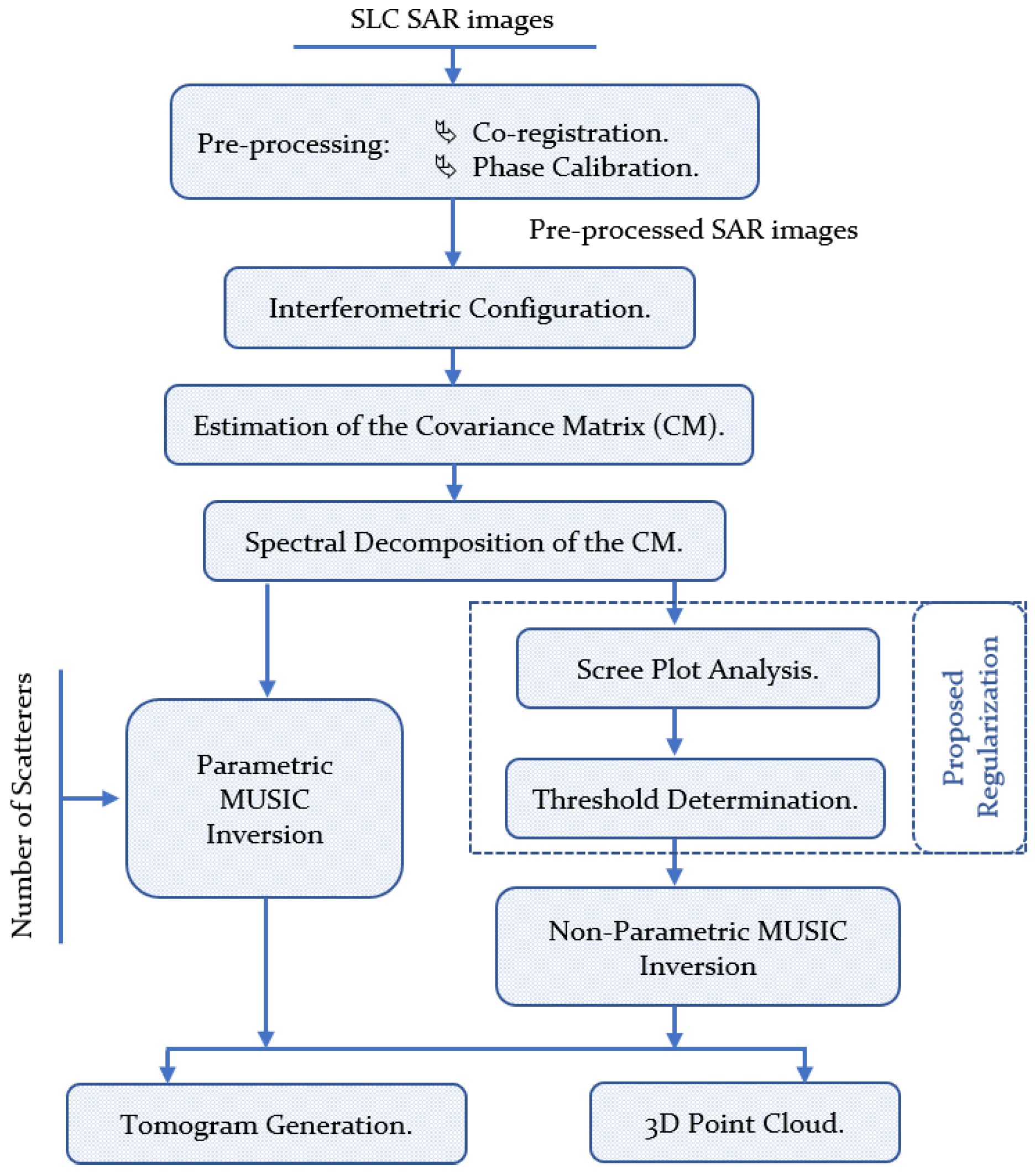
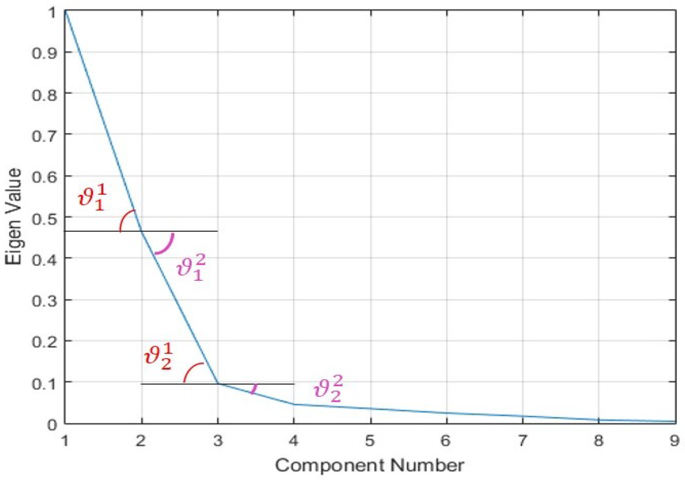
2.2. Proposed Method

Our methodology is schematized by the flowchart in Figure 2. In this section, we describe the main blocks that highlight our contributions.

Under the assumption of accurate inversion, subspace-based algorithms achieve maximum super-resolution capability with the correct number of scatterers $N_s$. The use of Eigen decomposition can be explored in this regard. Mathematically, if the sensing matrix $\mathit{A}$ has a uniform baseline spacing (i.e., the columns are linearly independent), and the reflectivity correlation matrix ${\mathit{R}}_{\gamma }$ is non-singular and positive definite (i.e., each target bin is independent), the data covariance matrix ${\mathit{R}}_g$ is a Hermitian full-rank matrix $({\mathit{R}}_g^H={\mathit{R}}_g)$ and has N positive real eigenvalues sorted according to their significance ${\lambda }_1>{\lambda }_2>\cdots >{\lambda }_N$. It can be expressed as follows:

$${\widehat{\mathit{R}}}_g=\sum _{i=1}^N{\lambda }_i{\mathit{u}}_i{\mathit{u}}_i^T=\mathit{U}\mathsf{\Lambda }{\mathit{U}}^T$$

(11)

where $\mathit{U}$ is an orthogonal matrix, whose ith column is an eigenvector ${\mathit{u}}_i$ (note that ${\mathit{u}}_i^T{\mathit{u}}_i=0$ for $i\ne j$), and $\mathsf{\Lambda }$ is a diagonal matrix, whose ith diagonal element ${\lambda }_i$ is an eigenvalue.

Establishing the boundary between the signal and noise subspaces automatically by exploring the properties of the eigenvalues can have a beneficial impact on MN and MUSIC reconstructions. In this regard, similar to TSVD [40], a threshold $T_s$ can be set as a form of regularization. It aims to control the amount of useful information involved in the separation process while taking into account the presence of noise in the data. Consequently, the ill-posed problem in (2) becomes well-posed, and its solution approaches the original one with good precision. Similar to Tikhonov regularization [41], which is known as one of the most common approaches for resolving ill-posed problems, the number of scatterers $N_s$ for a single azimuth–range pixel can be determined as follows:

$$N_s=min\left\{k\right\}suchas\frac{{\sum }_{i=1}^k{\lambda }_i}{Trace(\Lambda )}>T_s$$

(12)

$N_s$ is, in this case, the smallest value of k $(k=1,\cdots ,N)$, for which the desired cumulative percentage of variance is exceeded. Considering the threshold $T_s$ as a functional regularization parameter, the behavior of the eigenvalues is analyzed in order to control the relevant properties to be preserved.

For the sake of generality, a variety of thresholds can be chosen; yet, no evaluation approach exists that involves a certain degree of subjectivity in the choice of $T_s$ value. Depending on the data set’s particularity and the application’s practical detail requirements, effective cut-off levels are often in the range of $70\%$ to $95\%$ of the total variation cumulative percentage [42]. One way to determine the $T_s$ value is by analyzing the scree graph [43,44], which is a plot of eigenvalue ${\lambda }_i$ against component number i. The position of the sharpest ‘elbow’ on the diagram is sought to determine the value of $T_s$.

From this graphical representation, the changes in slopes ${\vartheta }^1$ (left-side angle) and ${\vartheta }^2$ (right-side angle) from steep to shallow for each point joining two consecutive straight lines (see Figure 3) can be calculated by looking for the first two subsequent eigenvalues that are nearly equal. The testing procedure starts from the graphical point corresponding to the second largest component number and stops at the graphical point corresponding to the penultimate component number. The Cattell formulation for ${\vartheta }_l^1$ and ${\vartheta }_l^2$, where l varies from 2 to $(N-1)$, is

$${\vartheta }_l^1=arctan({\lambda }_{l-1}-{\lambda }_l)$$

(13a)

$${\vartheta }_l^2=arctan({\lambda }_l-{\lambda }_{l+1})$$

(13b)

The determination of the cut-off threshold from ${\vartheta }^1$ and ${\vartheta }^2$ slopes typifies the amount of total cumulative variance accounted for by the uncorrupted data. It can be expressed as

$$T_s=1-\frac{arg{max}_l\left\{\right|{\vartheta }_l^1-{\vartheta }_l^2\left|\right\}}{N}$$

(14)

To sum up, the proposed regularization provides an accurate estimate of the cut-off threshold and number of scatterers by applying Equations (12) and (14), respectively. This automatic approach allows the tomographic inversion according to Equation (5) without the need for any external unknown parameters, transforming the MUSIC estimator into a non-parametric method. Note that this regularization can be applied to the Minimum-Norm method as well.

3. Results and Discussion

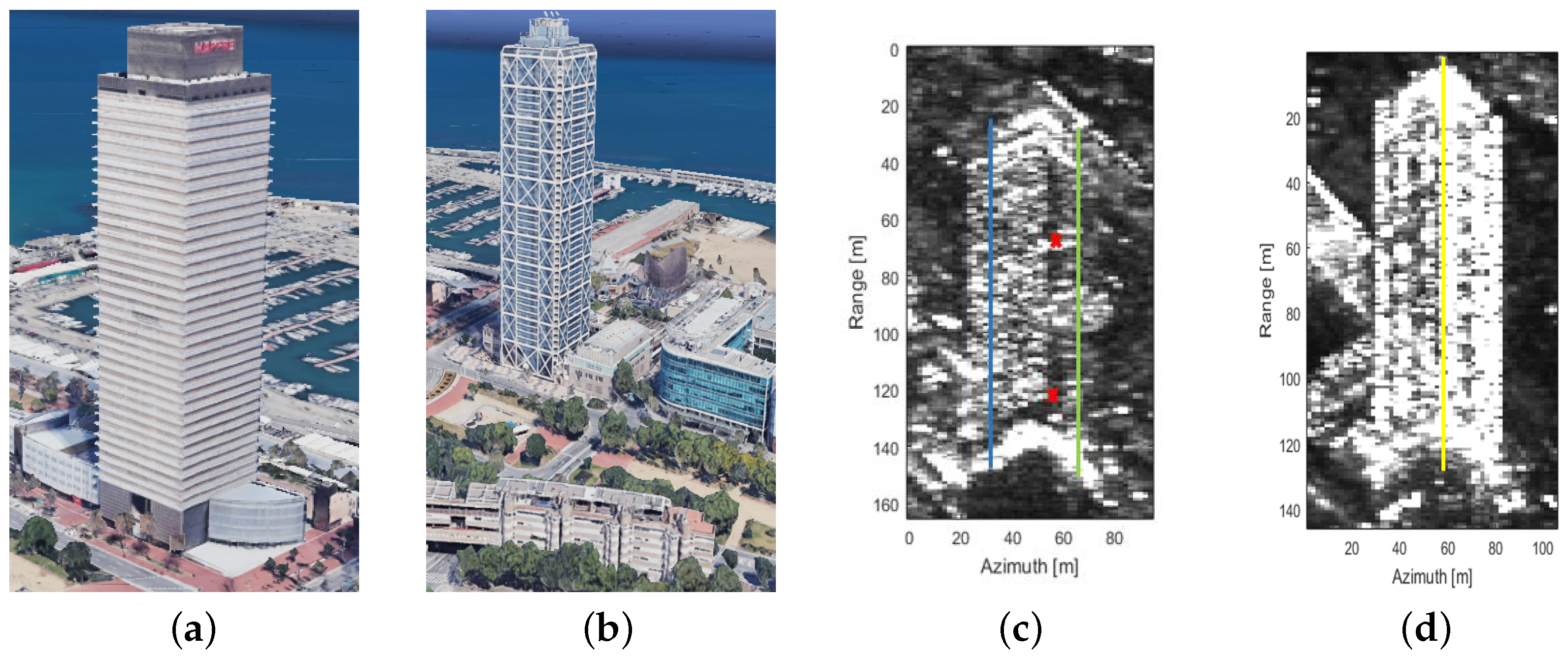
3.1. Data Sets

In this section, the performances of the proposed method are analyzed through its application on two data sets covering an urban area in Barcelona, Spain, acquired by TSX satellite. The sensor parameters are presented in

Table 1. TSX parameters of our data sets.

Parameters	Quantity
	Data Set 1	Data Set 2
Site	Barcelona (Spain)
Acquisition mode	StripMap
Wavelength	0.031 (m)
View angle	35°
Range Distance	618 (km)
Baseline Spam	157.74 (m)	506.32 (m)
Rayleigh Elevation resolution	60.80 (m)	18.94 (m)
Height resolution	34.88 (m)	10.87 (m)
Number of images	9	28

. The structures under study are the tall man-made buildings “Mapfre Tower” and “Arts Hotel”, located at latitudes of 41°23′16″N and 41°23′12″N, along with longitudes of 2°11′51″E and 2°11′4″E, respectively, with a height of 154 m each. The two buildings have distinct outer perimeter structures that backscatter differently; the Mapfre external is constructed from a concrete–steel composite while the Arts Hotel facade coating is a mixture of glass curtain wall, aluminum, and steel. Their Google Earth optical images and SAR amplitude maps are displayed in Figure 4.

According to the information gathered from visual inspection, the two buildings are localized in areas where single, double, and triple scatterers should be detected. We selected the most challenging azimuthal profiles (see Figure 4c,d) for detailed analysis in our study. In each resolution cell, the main scatterer belongs to the visible facade facing the sensor, while the second and third scatterers, if identified, represent the ground and low-elevated buildings surrounding the main structure.

The SAR images were pre-processed according to the following procedure:

• A geometric registration on a sub-pixel scale of all images according to a reference one was carried out.
• A phase difference was accomplished by subtracting the phase of the master image from all the images in the data set.
• A phase correction step was completed by subtracting the phase of a ground point that we selected as a reference, which made it possible to compensate the atmospheric phase (note that the atmospheric phase screen is considered constant over the whole image due to the limitation of the scene dimension).

3.2. Performance Metrics

To quantitatively measure how well the estimated $N_s$ (from Equation (12)) via our graphical approach approximates the actual number of scatterers, the R-squared [45] and Completeness [17] metrics can be used.

R-squared is the most common metric that assesses the performances of a given model in machine learning applications [46]. Its values lie between 0 and 1; the higher the value, the better the model. The calculation formula is

$$R_q^2=1-\frac{{\sum }_i{(h_i-{\widehat{h}}_i)}^2}{{\sum }_i{(h_i-{\overline{h}}_i)}^2}$$

(15)

where $h_i$, ${\widehat{h}}_i$, and ${\overline{h}}_i$ account for the ground truth, the estimated, and the mean height values, respectively.

Completeness measures the average distortion between the ground truth and the recovered reflectivity profiles [47]. The lower the value, the better the reconstruction performance. Its expression is given by

$$C_t=\frac{1}{M}\sum _{i=1}^M\underset{k}{min}\mathrm{dist}(\widehat{\gamma }\left(h_k\right),\gamma \left(h_i\right))$$

(16)

where $\widehat{\gamma }$ and $\gamma$ represent the estimated and ground truth reflectivities, respectively, while dist accounts for the distortion measure calculated using the Manhattan distance.

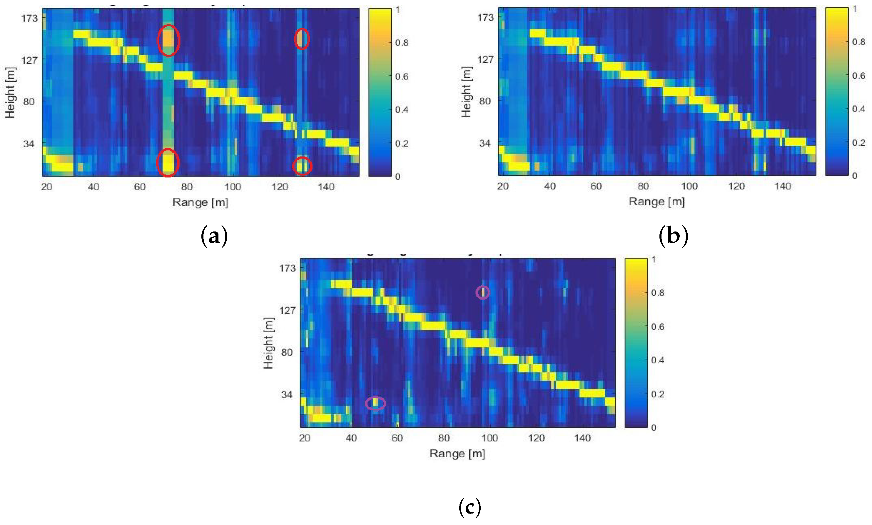
3.3. Analysis and Evaluation

Our analysis started with the need to set up the right regularization parameter for each resolution cell. In the first attempt to study the effect of this threshold on the reconstructed reflectivity profiles, we generated three tomograms using the first data set (see Figure 4a,c) by applying the regularized MUSIC estimator, on which the value of $T_s$ (in Equation (12)) was set to 85%, 90%, and 95%, respectively. According to the selected blue azimuthal line shown in Figure 4c, the expected tomogram should provide a linear form describing the gradation of the elevation values from approximately 0 m to 155 m. The findings displayed in Figure 5 showed that the 85% threshold creates some discontinuities in the linear form. In fact, the red circles (in Figure 5a) represent retrieved resolution cells whose elevation values are completely erroneous. This is due to the wrong separation between the signal and the noise subspaces. On the contrary, the 90% threshold leads to a good precision on the scatterers’ localization within the reflectivity profiles (see Figure 5b). Strangely, by setting up a higher value for $T_s$ (95%), inconsistencies appeared (see the purple circles in Figure 5c), where some reflectivity profiles started exhibiting the presence of sidelobes.

The current analysis leads to the conclusion that increasing the value of $T_s$ does not guarantee an improvement. To further investigate that, we calculated the R-squared metric over four random azimuthal lines and plotted their evolution as a function of $T_s$. The results displayed in Figure 6 show that maximum accuracy can be reached at a specific value of $T_s$ within the range of 75% to 95% for each profile. It is also clear that the reconstruction performance may witness considerable variations (deterioration or improvement) between closely spaced $T_s$ values. As a result, the best-case scenario involves the coordinates of the maximum R-squared value.

For the purpose of adequately selecting the right value of $T_s$, an automatic approach described in Section 2.2 has been established. An assessment of its impact on the inverted profiles was first carried out on two azimuth–range resolution cells, whose locations were marked on the mean amplitude map of Figure 4c. The first cell belongs to the bottom part, and the second cell to the top part, of the Mapfre building facade that manifests weak backscattering capability and strong noise presence. Their scree graphs were analyzed by calculating for each Eigen component the angles ${\vartheta }^1$ and ${\vartheta }^2$ and, therefore, deducing the value of $T_s$. The measures of one resolution cell are collected in

Table 2. ${\vartheta }^1$ and ${\vartheta }^2$ values for one resolution cell.

l	${\mathit{\vartheta }}_{\mathit{l}}^1$	${\mathit{\vartheta }}_{\mathit{l}}^2$	$|{\mathit{\vartheta }}_{\mathit{l}}^1-{\mathit{\vartheta }}_{\mathit{l}}^2|$
2	42.1279	3.1282	38.9998
3	3.1282	0.8589	2.2692
4	0.8589	0.6460	0.2129
5	0.6460	0.4669	0.1791
6	0.4669	0.1017	0.3651
7	0.1017	0.1222	0.0204
8	0.1222	0.0928	0.0294
$T_s$ value			88.89

. By visual comparison between the reconstructed profiles from classical MUSIC, BIC-MUSIC, Minimum-Norm, Regularized Minimum-Norm, and the proposed regularized MUSIC shown in Figure 7a,b, it is observed that all the methods failed to estimate the height of the main scatterer in both cases, while our proposed method succeeded (the height of the dominant scatterer coincides with the ground truth height marked by the red vertical line). Additionally, the proposed regularization applied to the Minimum-Norm approach showed some improvement compared to the standard version, since it achieved good reconstruction of the second resolution cell (better localization of the main scatterer is remarked in Figure 7b.4 compared with Figure 7b.3). The latter observation attests to the performance of the proposed regularization approach.

To further study the effectiveness of the proposed method, three azimuthal lines have been considered, covering two main portions of the Mapfre tower (Figure 4c) and the visible border of the Arts Hotel tower (Figure 4d). The ground truth height for the buildings under study was provided by Google Earth. The tomograms are generated by applying a standard MUSIC, BIC-MUSIC, Minimum-Norm, Regularized Minimum-Norm, and the proposed non-parametric MUSIC; the results are displayed in Figure 8, Figure 9 and Figure 10. In all tomograms, the reconstructed reflectivity profiles in the range–height plane exhibit a similar form; the main scatterer’s elevation in a resolution cell decreases with the increase in the range value—this attainment relates to the building’s height according to the SAR configuration.

The blue line in Figure 4c wraps the Mapfre tower facade, whose backscattering reflectivity is the strongest. By analyzing the obtained tomograms of Figure 8, we observe that the standard MUSIC, Minimum-Norm, and BIC-MUSIC methods show signs of sidelobes’ effects and the pixels located on the tower’s top side (the range interval [20 m, 30 m]) exhibit inaccurate height reconstruction. Although, we can point out that the height in this portion is better estimated by our regularized Minimum-Norm and MUSIC estimators. Their tomograms also attest to their capability to undoubtedly reduce the sidelobes’ amplitudes. Note that in the range portion from 20 m to 150 m, the number of scatterers is assumed equal to 2 for the standard MUSIC since it covers an overlaid area.

The tomograms obtained by inverting the green line in Figure 4c, covering the Mapfre building facade that exhibits poor backscattering power, support the previous findings. In this case, we can observe in Figure 9 that standard MUSIC and Minimum-Norm failed to reconstruct several reflectivity profiles within the considered line. On the other hand, the BIC-MUSIC and Regularized Minimum-Norm slightly improved the results. Fortunately, the proposed method succeeded in identifying the signal/noise barrier, leading to accurate height estimation with the exception of a few resolution cells where height inaccuracy persists.

Unlike the Mapfre structure, both visible facades of the Arts Hotel have similar backscattering brightness scales (see Figure 4d). Therefore, in our study, we selected an azimuthal profile that covers the corner facing the sensor. The tomograms of Figure 10 show the results of inverting the yellow line in Figure 4d. We observe that the proposed method remarkably improves the returned reflectivity profiles, reducing sidelobes and outliers. Additionally, the resolution cells located at range values beyond 120 m cover a low elevation building surrounding the Arts Hotel structure. This portion is well reconstructed with the proposed approach compared with classical MUSIC and BIC-MUSIC. Unfortunately, both variants of the Minimum-Norm method perform poorly in this data set, especially the standard version, along the whole range axis. The divergent behavior of the same estimator is related to the distinct baseline configurations of our data sets, and the important PSF leakage (resulted in Figure 10c,d) is mainly due to the non-uniform orbits of the repeat-pass spaceborne SAR images. In fact, increasing their number and/or the baseline interval extent does not necessarily improve the accuracy of the estimated elevations.

The Cramer–Rao Lower Bound (CRLB) for our two data stacks is shown in Figure 11 as a function of the Signal-to-Noise Ratio (SNR). In each plot, we compare the actual baseline configuration variation with the ideal case scenario, which has a uniform separation between orbits. In the first data set, the drop in the CRLB is negligible for all SNR levels (see Figure 11a). This indicates that the height estimation accuracy is almost unaffected by the non-uniform distribution of orbits along the baseline axis. However, in the second data set, Figure 11b) shows that the CRLB drops by 0.4 m when the SNR is equal to 1 dB, and it further decreases with increasing SNR. From this analysis, we can confidently conclude that the difference in the tomographic reconstruction quality between the two data sets is mainly related to the system parameters, particularly the baseline separation and the view angle, as well as the noise level.

To assess the conclusions obtained from visual inspection of Figure 8, Figure 9 and Figure 10 quantitatively, we calculated the R-squared and completeness parameters. The results in

Table 3. R-squared and Completeness metrics.

Method	${\mathit{R}}_{\mathit{q}}^2$		${\mathit{C}}_{\mathit{t}}$
	Data Set 1	Data Set 2	Data Set 1	Data Set 2
Classical MUSIC	0.0734	0.8169	0.8309	0.1029
BIC-MUSIC	0.2150	0.2502	0.7476	0.2717
Minimum-Norm	0.0513	0.2528	0.8422	0.3765
Regularized Minimum-Norm	0.0874	0.3429	0.7811	0.2627
Proposed MUSIC	0.2246	0.8821	0.7002	0.0806

quantify the quality of the tomographic reconstruction by the five estimators. We can deduce that the proposed method has the highest value of $R_q^2$ and the smallest value of $C_t$ in both cases (data sets 1 and 2), which prove its superiority over the other four methods. Furthermore, we can establish from these findings that the regularized Minimum-Norm approach exhibits better performances compared with the standard version.

In summary, it is possible to confirm that the assumed number of scatterers may lead to biased 3D reconstruction via standard MUSIC and Minimum-Norm spectral estimators. Moreover, the estimation of $N_s$ via model selection schemas (in our study, the Bayesian Information Criterion, whose complexity penality is $C\left(N_s\right)=(N_s/2)·lnN$, was used) provides some improvement at the expense of computational cost. Additionally, its accuracy depends on the non-parametric method chosen in the first tomographic inversion. For this reason, we applied the compressive sensing method to estimate the scatterers’ height due to its super-resolution capability, aiming to provide the best estimation for the model selection algorithm. (note that a Matlab-based modeling system for convex optimization, named “cvx” toolbox, was used to solve the minimization problem of the CS-based sparse reconstruction [48,49]). Nevertheless, the presented tomograms (in Figure 8, Figure 9 and Figure 10) demonstrated the improvement of the regularized version of Minimum-Norm method and the good performance of the proposed non-parametric MUSIC in reducing the PSF leakage, correcting the mislocalization of scatterers having weak backscattering properties, all while automatically estimating the number of scatterers from the scree diagram analysis.

This deduction can also be made from Figure 12 and Figure 13, where the 3D views of the Mapfre and Arts Hotel height maps have been generated for the five algorithms. The processing has been applied to all pixels belonging to the buildings, and the computation includes a peak detector of the main scatterer in the retrieved reflectivity profiles. From the results, it is clear that our proposed improved regularized MUSIC is less affected by outliers in both studied cases, which attests to its ability to improve the scatterers’ height estimation. We can conclude that the performance of the proposed regularization method depends on the accuracy of the estimated multidimensional covariance matrix. The lower the error in the estimation, the better the results. On the other hand, the results of the other methods show high sensitivity to various factors such as baseline separation, view angle, and noise level. This is evident from the reconstructions obtained using the Standard MUSIC estimator, BIC-MUSIC estimator, and Minimum-Norm estimator on the second data set (see Figure 10 and Figure 13). In contrast, the proposed method exhibits a more robust behavior.

4. Conclusions

This research study aimed to improve tomographic SAR inversion using subspace-based methods—specifically, the MUSIC estimator—by developing an automatic method for determining the number of scatterers in each resolution cell. The regularization step involved setting a threshold based on scree graph analysis, which classifies the proposed MUSIC variant as a non-parametric method. The proposed approach was evaluated using two stacks of TSX images over the city of Barcelona, Spain, with a focus on analyzing the localization of scatterers in the height axis and reducing PSF leakage.

The evaluation of the regularization step was conducted using the R-squared and Completeness metrics, which showed that maximum accuracy for height estimation was achieved when the proper number of scatterers was established. The improved regularized MUSIC was compared with other subspace-based estimation methods including Standard MUSIC, BIC-MUSIC, Minimum-Norm, and Regularized Minimum-Norm estimators. The results showed that the proposed method had a strong capability to reduce the sidelobes’ effects and improve the precision of height estimation for several profiles. The proposed estimator also demonstrated its robustness in areas with weak backscattering properties and strong noise presence for different data stacks configurations.

It is important to note that the proposed method can be extended to 4D TomoSAR for the retrieval of deformation maps and also combined with polarimetric decomposition for the retrieval of reflectivity maps in vegetated areas. Overall, the findings suggest that the improved regularized MUSIC estimator has significant potential to enhance the accuracy and precision of tomographic SAR inversion.

References

1. Jordan, R.L. The Seasat-A synthetic aperture radar system. IEEE J. Ocean. Eng. 1980, 5, 154–164. [Google Scholar] [CrossRef]
2. Wei, L.; Balz, T.; Liao, M.; Zhang, L. TerraSAR-X StripMap Data Interpretation of Complex Urban Scenarios with 3D SAR Tomography. J. Sens. 2014, 2014, 386753. [Google Scholar] [CrossRef] [Green Version]
3. Lavalle, M.; Hawkins, B.; Hensley, S. Tomographic imaging with UAVSAR: Current status and new results from the 2016 AfriSAR campaign. In Proceedings of the 2017 IEEE International Geoscience and Remote Sensing Symposium (IGARSS), Fort Worth, TX, USA, 23–28 July 2017; pp. 2485–2488. [Google Scholar] [CrossRef]
4. Moreira, A.; Prats-Iraola, P.; Younis, M.; Krieger, G.; Hajnsek, I.; Papathanassiou, K.P. A tutorial on synthetic aperture radar. IEEE Geosci. Remote Sens. Mag. 2013, 1, 6–43. [Google Scholar] [CrossRef] [Green Version]
5. Fornaro, G.; Serafino, F.; Soldovieri, F. Three-dimensional focusing with multipass SAR data. IEEE Trans. Geosci. Remote Sens. 2003, 41, 507–517. [Google Scholar] [CrossRef]
6. Reigber, A.; Moreira, A. First demonstration of airborne SAR tomography using multibaseline L-band data. IEEE Trans. Geosci. Remote Sens. 2000, 38, 2142–2152. [Google Scholar] [CrossRef]
7. Gini, F.; Lombardini, F.; Montanari, M. Layover solution in multibaseline SAR interferometry. IEEE Trans. Aerosp. Electron. Syst. 2002, 38, 1344–1356. [Google Scholar] [CrossRef]
8. Stoica, P.; Moses, R. Introduction to Spectral Analysis; Prentice Hall: Hoboken, NJ, USA, 1997. [Google Scholar]
9. Fornaro, G.; Lombardini, F.; Pauciullo, A.; Reale, D.; Viviani, F. Tomographic Processing of Interferometric SAR Data: Developments, applications, and future research perspectives. IEEE Signal Process. Mag. 2014, 31, 41–50. [Google Scholar] [CrossRef]
10. Rambour, C.; Budillon, A.; Johnsy, A.C.; Denis, L.; Tupin, F.; Schirinzi, G. From Interferometric to Tomographic SAR: A Review of Synthetic Aperture Radar Tomography-Processing Techniques for Scatterer Unmixing in Urban Areas. IEEE Geosci. Remote Sens. Mag. 2020, 8, 6–29. [Google Scholar] [CrossRef]
11. Budillon, A.; Evangelista, A.; Schirinzi, G. SAR tomography from sparse samples. In Proceedings of the 2009 IEEE International Geoscience and Remote Sensing Symposium, Cape Town, South Africa, 12–17 July 2009; Volume 4, pp. IV-865–IV-868. [Google Scholar] [CrossRef]
12. Zhu, X.X.; Bamler, R. Tomographic SAR Inversion by L1-Norm Regularization—The Compressive Sensing Approach. IEEE Trans. Geosci. Remote Sens. 2010, 48, 3839–3846. [Google Scholar] [CrossRef] [Green Version]
13. Budillon, A.; Evangelista, A.; Schirinzi, G. Three-dimensional SAR focusing from multipass signals using compressive sampling. IEEE Trans. Geosci. Remote Sens. 2010, 49, 488–499. [Google Scholar] [CrossRef]
14. Zhu, X.X.; Bamler, R. Superresolving SAR tomography for multidimensional imaging of urban areas: Compressive sensing-based TomoSAR inversion. IEEE Signal Process. Mag. 2014, 31, 51–58. [Google Scholar] [CrossRef]
15. Adeli, S.; Akhoondzadeh Hanzaei, M.; Zakeri, S. Very High Resolution Parametric and Non-Parametric Sartomography Methods for Monitoring Urban Areas Structures. J. Geomat. Sci. Technol. 2019, 8, 1–11. [Google Scholar]
16. Seker, I.; Lavalle, M. Tomographic Performance of Multi-Static Radar Formations: Theory and Simulations. Remote Sens. 2021, 13, 737. [Google Scholar] [CrossRef]
17. D’Hondt, O.; López-Martínez, C.; Guillaso, S.; Hellwich, O. Nonlocal Filtering Applied to 3-D Reconstruction of Tomographic SAR Data. IEEE Trans. Geosci. Remote Sens. 2018, 56, 272–285. [Google Scholar] [CrossRef]
18. Aghababaee, H.; Ferraioli, G.; Schirinzi, G.; Pascazio, V. Regularization of SAR Tomography for 3-D Height Reconstruction in Urban Areas. IEEE J. Sel. Top. Appl. Earth Obs. Remote Sens. 2019, 12, 648–659. [Google Scholar] [CrossRef]
19. Lombardini, F.; Gini, F.; Matteucci, P. Application of array processing techniques to multibaseline InSAR for layover solution. In Proceedings of the 2001 IEEE Radar Conference (Cat. No.01CH37200), Atlanta, GA, USA, 3 May 2001; pp. 210–215. [Google Scholar] [CrossRef]
20. Guillaso, S.; Reigber, A. Scatterer characterisation using polarimetric SAR tomography. In Proceedings of the International Geoscience and Remote Sensing Symposium, Seoul, Republic of Korea, 25–29 July 2005; Volume 4, p. 2685. [Google Scholar]
21. Sauer, S.; Ferro-Famil, L.; Reigber, A.; Pottier, E. Polarimetric Dual-Baseline InSAR Building Height Estimation at L-Band. IEEE Geosci. Remote Sens. Lett. 2009, 6, 408–412. [Google Scholar] [CrossRef]
22. Kong, L.; He, X.; Xu, X. A Fully-Polarized Unitary MUSIC for Polarimetric SAR Tomography. In Proceedings of the 2019 International Conference on Electromagnetics in Advanced Applications (ICEAA), Granada, Spain, 9–13 September 2019; pp. 0964–0967. [Google Scholar] [CrossRef]
23. Ren, X.; Qin, Y.; Tian, L. Three-dimensional imaging algorithm for tomography SAR based on multiple signal classification. In Proceedings of the 2014 IEEE International Conference on Signal Processing, Communications and Computing (ICSPCC), Guilin, China, 5–8 August 2014; pp. 120–123. [Google Scholar] [CrossRef]
24. Martín-del Campo-Becerra, G.D.; Serafín-García, S.A.; Reigber, A.; Ortega-Cisneros, S. Parameter selection criteria for Tomo-SAR focusing. IEEE J. Sel. Top. Appl. Earth Obs. Remote Sens. 2020, 14, 1580–1602. [Google Scholar] [CrossRef]
25. Naghavi, A.; Fazel, M.S.; Beheshti, M.; Yazdian, E. A sequential MUSIC algorithm for scatterers detection in SAR tomography enhanced by a robust covariance estimator. Digit. Signal Process. 2022, 128, 103621. [Google Scholar] [CrossRef]
26. Bamler, R.; Hartl, P. Synthetic aperture radar interferometry. Inverse Probl. 1998, 14, R1–R54. [Google Scholar] [CrossRef]
27. Xu, G.; Gao, Y.; Li, J.; Xing, M. InSAR Phase Denoising: A Review of Current Technologies and Future Directions. IEEE Geosci. Remote Sens. Mag. 2020, 8, 64–82. [Google Scholar] [CrossRef] [Green Version]
28. Guillaso, S.; D’Hondt, O.; Hellwich, O. SAR tomography with reduced number of tracks: Urban object reconstruction. In Proceedings of the 2015 IEEE International Geoscience and Remote Sensing Symposium (IGARSS), Milan, Italy, 26–31 July 2015; pp. 2919–2922. [Google Scholar] [CrossRef]
29. Budillon, A.; Schirinzi, G. Support detection for SAR tomographic reconstructions from compressive measurements. Sci. World J. 2015, 2015, 949807. [Google Scholar] [CrossRef] [PubMed] [Green Version]
30. Zhu, X.X.; Bamler, R. Very High Resolution Spaceborne SAR Tomography in Urban Environment. IEEE Trans. Geosci. Remote Sens. 2010, 48, 4296–4308. [Google Scholar] [CrossRef] [Green Version]
31. Schmidt, R. Multiple emitter location and signal parameter estimation. IEEE Trans. Antennas Propag. 1986, 34, 276–280. [Google Scholar] [CrossRef] [Green Version]
32. Dănișor, C.; Fornaro, G.; Pauciullo, A.; Reale, D.; Datcu, M. Super-resolution multi-look detection in SAR tomography. Remote Sens. 2018, 10, 1894. [Google Scholar] [CrossRef] [Green Version]
33. Chen, Z.; Gokeda, G.; Yu, Y. Introduction to Direction-of-Arrival Estimation; Artech House: London, UK, 2010. [Google Scholar]
34. Foutz, J.; Spanias, A.; Banavar, M.K. Narrowband direction of arrival estimation for antenna arrays. Synth. Lect. Antennas 2008, 3, 1–76. [Google Scholar]
35. Omati, M.; Sahebi, M.R.; Aghababaei, H. Evaluation of nonparametric SAR tomography methods for urban building reconstruction. IEEE Geosci. Remote Sens. Lett. 2021, 19, 1–5. [Google Scholar] [CrossRef]
36. Pauciullo, A.; De Maio, A.; Perna, S.; Reale, D.; Fornaro, G. Detection of Partially Coherent Scatterers in Multidimensional SAR Tomography: A Theoretical Study. IEEE Trans. Geosci. Remote Sens. 2014, 52, 7534–7548. [Google Scholar] [CrossRef]
37. Budillon, A.; Schirinzi, G. GLRT Based on Support Estimation for Multiple Scatterers Detection in SAR Tomography. IEEE J. Sel. Top. Appl. Earth Obs. Remote Sens. 2016, 9, 1086–1094. [Google Scholar] [CrossRef]
38. Hansen, M.H.; Yu, B. Model Selection and the Principle of Minimum Description Length. J. Am. Stat. Assoc. 2001, 96, 746–774. [Google Scholar] [CrossRef]
39. Ferretti, A.; Bianchi, M.; Prati, C.; Rocca, F. Higher-order permanent scatterers analysis. EURASIP J. Adv. Signal Process. 2005, 2005, 609604. [Google Scholar] [CrossRef] [Green Version]
40. Fornaro, G.; Lombardini, F.; Serafino, F. Three-dimensional multipass SAR focusing: Experiments with long-term spaceborne data. IEEE Trans. Geosci. Remote Sens. 2005, 43, 702–714. [Google Scholar] [CrossRef]
41. Tihonov, A.N. Solution of incorrectly formulated problems and the regularization method. Soviet Math. 1963, 4, 1035–1038. [Google Scholar]
42. Jolliffe, I.T. Principal Component Analysis, 2nd ed.; Springer: New York, NY, USA, 2002. [Google Scholar] [CrossRef]
43. Craddock, J.M.; Flood, C.R. Eigenvectors for representing the 500 mb geopotential surface over the Northern Hemisphere. Q. J. R. Meteorol. Soc. 1969, 95, 576–593. [Google Scholar] [CrossRef]
44. Farmer, S.A. An Investigation into the Results of Principal Component Analysis of Data Derived from Random Numbers. J. R. Stat. Soc. Ser. (Stat.) 1971, 20, 63–72. [Google Scholar] [CrossRef]
45. Hadj-Rabah, K.; Schirinzi, G.; Daoud, I.; Hocine, F.; Belhadj-Aissa, A. Spatio-Temporal Filtering Approach for Tomographic SAR Data. IEEE Trans. Geosci. Remote Sens. 2023, 61, 1–13. [Google Scholar] [CrossRef]
46. Vaid, K.; Ghose, U. Predictive Analysis of Manpower Requirements in Scrum Projects Using Regression Techniques. Procedia Comput. Sci. 2020, 173, 335–344. [Google Scholar] [CrossRef]
47. Liu, W.; Budillon, A.; Pascazio, V.; Schirinzi, G.; Xing, M. Performance Improvement for SAR Tomography Based on Local Plane Model. IEEE J. Sel. Top. Appl. Earth Obs. Remote Sens. 2022, 15, 2298–2310. [Google Scholar] [CrossRef]
48. Grant, M.; Boyd, S. CVX: Matlab Software for Disciplined Convex Programming, Version 2.1. 2014. Available online: http://cvxr.com/cvx (accessed on 13 March 2023).
49. Grant, M.; Boyd, S. Graph implementations for nonsmooth convex programs. In Recent Advances in Learning and Control; Blondel, V., Boyd, S., Kimura, H., Eds.; Lecture Notes in Control and Information Sciences; Springer: Berlin/Heidelberg, Germany, 2008; pp. 95–110. [Google Scholar]
Figure 1. TomoSAR geometry.
Remotesensing 15 01599 g001
Figure 2. Block diagram of the proposed approach.
Remotesensing 15 01599 g002
Figure 3. An example of a scree plot.
Remotesensing 15 01599 g003
Figure 4. Location of (a) the “Mapfre” and (b) the “Arts Hotel” towers on Google Earth. (c,d) Mean amplitude maps with considered profiles and resolution cells.
Remotesensing 15 01599 g004
Figure 5. Generated tomograms using the proposed estimator with (a) 85%, (b) 90%, and (c) 95% thresholds.
Remotesensing 15 01599 g005
Figure 6. Plots of the R-squared metric as a function of T s for different reconstructed azimuthal lines.
Remotesensing 15 01599 g006
Figure 7. Reflectivity profiles for two azimuth–range pixels (a,b) using the (1) Standard MUSIC estimator, (2) BIC-MUSIC estimator, (3) Minimum-Norm estimator, (4) Regularized Minimum-Norm estimator, and (5) proposed regularized MUSIC estimator.
Remotesensing 15 01599 g007
Figure 8. Tomograms of the blue azimuthal line generated by the (a) Standard MUSIC estimator, (b) BIC-MUSIC estimator, (c) Minimum-Norm estimator, (d) Regularized Minimum-Norm estimator, and (e) proposed non-parametric MUSIC estimator.
Remotesensing 15 01599 g008
Figure 9. Tomograms of the green azimuthal line generated by the (a) Standard MUSIC estimator, (b) BIC-MUSIC estimator, (c) Minimum-Norm estimator, (d) Regularized Minimum-Norm estimator, and (e) proposed non-parametric MUSIC estimator.
Remotesensing 15 01599 g009
Figure 10. Tomograms of the yellow azimuthal line generated by the (a) Standard MUSIC estimator, (b) BIC-MUSIC estimator, (c) Minimum-Norm estimator, (d) Regularized Minimum-Norm estimator, and (e) proposed non-parametric MUSIC estimator.
Remotesensing 15 01599 g010
Figure 11. Cramer–Rao Lower Bound for (a) nine orbits of data set 1 and (b) twenty-eight orbits of data set 2.
Remotesensing 15 01599 g011
Figure 12. Three-dimensional views of the Mapfre height maps generated by the (a) Standard MUSIC estimator, (b) BIC-MUSIC estimator and (c) Minimum-Norm estimator, (d) Regularized Minimum-Norm estimator, and (e) the proposed non-parametric MUSIC estimator.
Remotesensing 15 01599 g012
Figure 13. Three-dimensional views of the Arts Hotel height maps generated by the (a) Standard MUSIC estimator, (b) BIC-MUSIC estimator and (c) Minimum-Norm estimator, (d) Regularized Minimum-Norm estimator, and (e) the proposed non-parametric MUSIC estimator.
Remotesensing 15 01599 g013