Study of Land Cover Change in the City with the Fastest Economic Growth in China (Hefei) from 2000 to 2020 Based on Google Earth Engine Platform
Abstract
1. Introduction
2. Materials and Methods
2.1. Study Area
2.2. Data Acquisition
Data Sources
2.3. Methodology
2.3.1. Technical Process
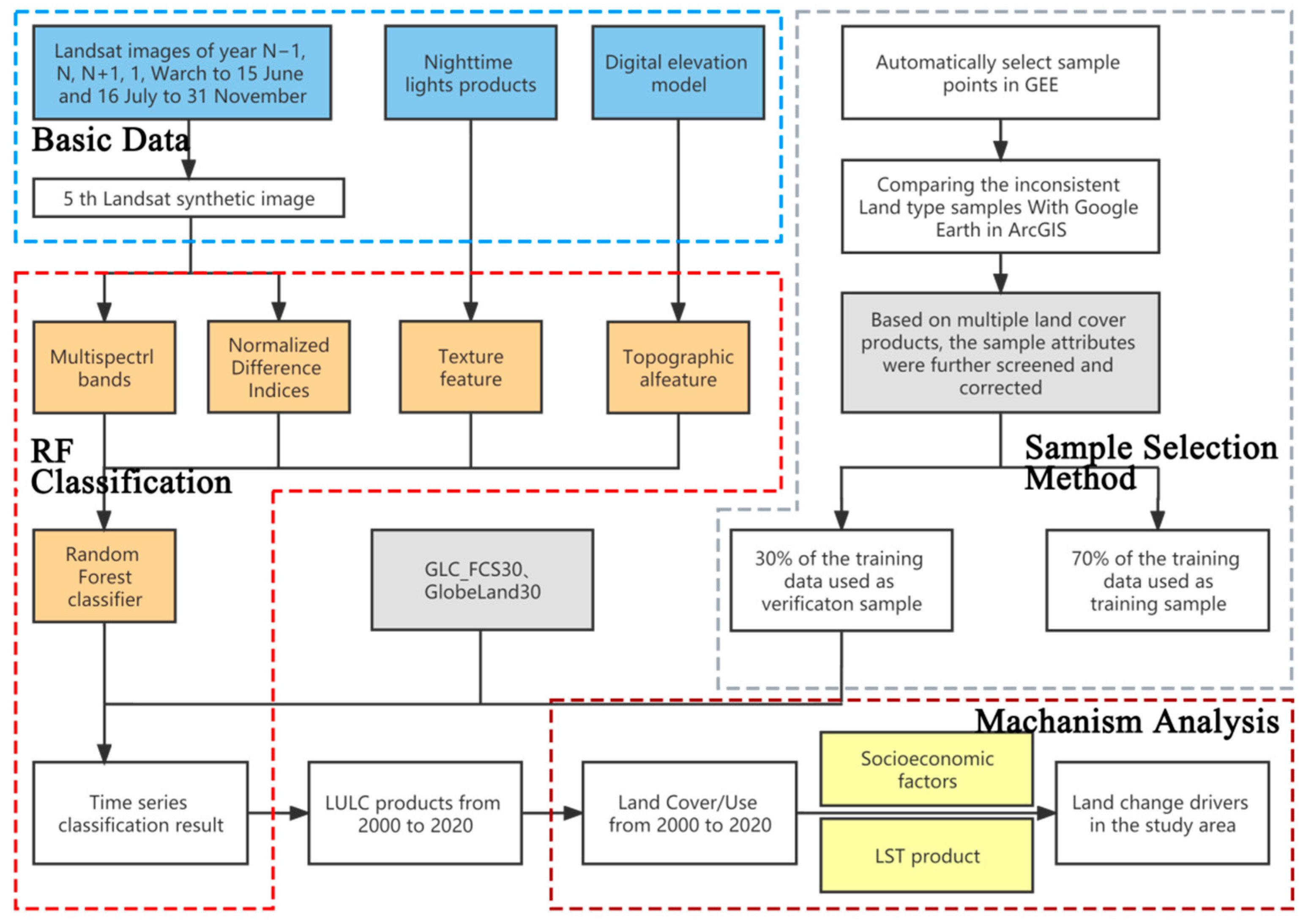
- With the support of the GEE platform, the cloud cover function was used to process the multi-year image datasets to obtain the composite image data of TOA products without cloud, snow, and shadow covering in the five periods from 2000 to 2020 (1999–2001, 2005–2007, 2010–2012, 2015–2017, and 2019–2020).
- The sample points were collected on GEE, filtered, and corrected with Google Earth high-resolution images. The training and validation samples were carefully deployed according to the “complete consistency” and “temporal stability” principles. The land cover attributes were extracted for the samples.
- Based on the Landsat series satellite images, a variety of data and normalized difference index were used as input parameters of the RF algorithm classifier. Then, the training samples were used to produce the land use classification result of the study area in the five periods.
- After obtaining the land use classification result of each period, the changes in various land features and the driving factors of LCC were analyzed.
2.3.2. Training Sample Point Selection
- According to the research interval (2000–2020), we selected the land cover products (e.g., GlobeLand30 and MCD12Q1.006) for stratified sampling based on the GEE platform. The remap function on GEE platform was used to remap the two images to the required feature types, and the stratified sample function was used to sample the images hierarchically.
- In the selected sample points, some error sample points appear in the sample data selected online affected by individual error pixels. Therefore, we need to further improve the sample data through the offline Google Earth platform test. In the process of classification, 70% of the collected sample points were used as training sample points, and 30% were used as verification sample points to verify the accuracy of classification. The numbers of selected images and sample points are shown in Figure 3.
2.3.3. Study Method
3. Results
3.1. Accuracy Assessment
3.2. Spatio–Temporal Variations in Land Cover
3.2.1. Spatio-Temporal Variations in Vegetation Coverage
3.2.2. Spatio-Temporal Variation in Water Body
3.2.3. Spatio-Temporal Variations in Built-Up Area
3.3. LCC of Driving Forces in Hefei
4. Discussion
5. Conclusions
Author Contributions
Funding
Data Availability Statement
Acknowledgments
Conflicts of Interest
References
- Cristina, G.; Joanne, C.W.; Michael, A.W. Optical remotely sensed time series data for land cover classification: A review. ISPRS-J. Photogramm. Remote Sens. 2016, 116, 55–72. [Google Scholar]
- Kavitha, A.V.; Srikrishna, A.; Satyanarayana, C. A Review on Detection of Land Use and Land Cover from an Optical Remote Sensing Image. IOP Conf. Ser. Mater. Sci. Eng. 2021, 1074, 12002. [Google Scholar] [CrossRef]
- Gorelick, N.; Hancher, M.; Dixon, M.; Ilyushchenko, S.; Thau, D.; Moore, R. Google Earth Engine: Planetary-scale geospatial analysis for everyone. Remote Sens. Environ. 2017, 202, 18–27. [Google Scholar] [CrossRef]
- Amani, M.; Ghorbanian, A.; Ahmadi, S.A.; Kakooei, M.; Brisco, B. Google Earth Engine Cloud Computing Platform for Remote Sensing Big Data Applications: A Comprehensive Review. Ieee J. Sel. Top. Appl. Earth Observ. Remote Sens. 2020, 13, 5326–5350. [Google Scholar] [CrossRef]
- Fu, D.J.; Xiao, H.; Su, F.Z.; Zhou, C.H.; Dong, J.W.; Zeng, Y.L.; Yan, K.; Li, S.W.; Wu, J.; Wu, W.Z.; et al. Remote sensing cloud computing platform development and Earth science application. J. Remote Sens. 2021, 25, 220–230. [Google Scholar]
- Xie, S.; Liu, L.; Zhang, X.; Yang, J.; Gao, Y. Automatic Land-Cover Mapping using Landsat Time-Series Data based on Google Earth Engine. Remote Sens. 2019, 11, 3023. [Google Scholar] [CrossRef]
- Kumar, L.; Mutanga, O. Google Earth Engine Applications Since Inception: Usage, Trends, and Potential. Remote Sens. 2018, 10, 1509. [Google Scholar] [CrossRef]
- Hansen, M.C.; Potapov, P.V.; Moore, R.; Hancher, M.; Turubanova, S.A.; Tyukavina, A.; Thau, D.; Stehman, S.V.; Goetz, S.J.; Loveland, T.R.; et al. High-Resolution Global Maps of 21st-Century Forest Cover Change. Science 2013, 342, 850–853. [Google Scholar] [CrossRef]
- Dong, J.; Xiao, X.; Menarguez, M.A.; Zhang, G.; Qin, Y.; Thau, D.; Biradar, C.; Iii, B.M. Mapping paddy rice planting area in northeastern Asia with Landsat 8 images, phenology-based algorithm and Google Earth Engine. Remote Sens. Environ. 2016. [Google Scholar] [CrossRef]
- Du, Z.; Yang, J.; Ou, C.; Zhang, T. Agricultural Land Abandonment and Retirement Mapping in the Northern China Crop-Pasture Band Using Temporal Consistency Check and Trajectory-Based Change Detection Approach. IEEE Trans. Geosci. Remote Sens. 2022, 60, 1–12. [Google Scholar] [CrossRef]
- Zhang, K.; Dong, X.; Liu, Z.; Gao, W.; Hu, Z.; Wu, G. Mapping Tidal Flats with Landsat 8 Images and Google Earth Engine: A Case Study of the China’s Eastern Coastal Zone circa 2015. Remote Sens. 2019, 11, 924. [Google Scholar] [CrossRef]
- Yang, W.; Qi, W.; Fang, J. Using Google Earth Engine to monitor co-seismic landslide recovery after the 2008 Wenchuan earthquake. Earth Surf. Dynam. Discuss. 2020. [Google Scholar] [CrossRef]
- DeVries, B.; Huang, C.; Armston, J.; Huang, W.; Jones, J.W.; Lang, M.W. Rapid and robust monitoring of flood events using Sentinel-1 and Landsat data on the Google Earth Engine. Remote Sens. Environ. 2020, 240, 111664. [Google Scholar] [CrossRef]
- Sazib, N.; Mladenova, I.; Bolten, J. Leveraging the Google Earth Engine for Drought Assessment Using Global Soil Moisture Data. Remote Sens. 2018, 10, 1265. [Google Scholar] [CrossRef]
- Shamshiri, R.; Eide, E.; Høyland, K.V. Spatio-temporal distribution of sea-ice thickness using a machine learning approach with Google Earth Engine and Sentinel-1 GRD data. Remote Sens. Environ. 2022, 270, 112851. [Google Scholar] [CrossRef]
- Qiao, Z.; Liu, L.; Qin, Y.; Xu, X.; Wang, B.; Liu, Z. The Impact of Urban Renewal on Land Surface Temperature Changes: A Case Study in the Main City of Guangzhou, China. Remote Sens. 2020, 12, 794. [Google Scholar] [CrossRef]
- Zhang, Y.; Hu, Q.; Zou, F. Spatio-Temporal Changes of Vegetation Net Primary Productivity and Its Driving Factors on the Qinghai-Tibetan Plateau from 2001 to 2017. Remote Sens. 2021, 13, 1566. [Google Scholar] [CrossRef]
- Liu, G.; Li, J.; Nie, P. Tracking the history of urban expansion in Guangzhou (China) during 1665–2017: Evidence from historical maps and remote sensing images. Land Use Pol. 2022, 112, 105773. [Google Scholar] [CrossRef]
- Tu, L.; Qin, Z.; Li, W.; Geng, J.; Yang, L.; Zhao, S.; Zhan, W.; Wang, F. Surface urban heat island effect and its relationship with urban expansion in Nanjing, China. J. Appl. Remote Sens. 2016, 10, 26037. [Google Scholar] [CrossRef]
- Nor, A.; Corstanje, R.; Harris, J.A.; Brewer, T. Impact of rapid urban expansion on green space structure. Ecol. Indic. 2017, 81, 274–284. [Google Scholar] [CrossRef]
- Zhang, Z.; Ling, Y.I.; Shunguang, H.U.; Liu, B.; Liu, F.; Zhao, X.; Wang, X.; Shi, L.; Jinyong, X.U.; Sisi, Y.U. Urban Expansion in China Based on Remote Sensing Technology:A Review. Chin. Geogr. Sci. 2018, 28, 727–743. [Google Scholar] [CrossRef]
- Gong, J.; Hu, Z.; Chen, W.; Liu, Y.; Wang, J. Urban expansion dynamics and modes in metropolitan Guangzhou, China. Land Use Pol. 2018, 72, 100–109. [Google Scholar] [CrossRef]
- Sun, Z.; Xu, R.; Du, W.; Wang, L.; Lu, D. High-Resolution Urban Land Mapping in China from Sentinel 1A/2 Imagery Based on Google Earth Engine. Remote Sens. 2019, 11, 752. [Google Scholar] [CrossRef]
- Sengupta, D.; Chen, R.S.; Meadows, M.E.; Choi, Y.R.; Banerjee, A.; Zilong, X. Mapping Trajectories of Coastal Land Reclamation in Nine Deltaic Megacities using Google Earth Engine. Remote Sens. 2019, 11, 2621. [Google Scholar] [CrossRef]
- Huang, H.; Chen, Y.; Clinton, N.; Wang, J.; Wang, X.; Liu, C.; Gong, P.; Yang, J.; Bai, Y.; Zheng, Y.; et al. Mapping major land cover dynamics in Beijing using all Landsat images in Google Earth Engine. Remote Sens. Environ. 2017, 202, 166–176. [Google Scholar] [CrossRef]
- Zhao, S. Rapid urban expansion and its ecological consequences in Shanghai, China. Front. Ecol. Environ. 2006, 4, 341–346. [Google Scholar] [CrossRef]
- Zhang, D.; Zhang, L. Land Cover Change in the Central Region of the Lower Yangtze River Based on Landsat Imagery and the Google Earth Engine: A Case Study in Nanjing, China. Sensors 2020, 20, 2091. [Google Scholar] [CrossRef] [PubMed]
- Yao, Y.L.; Liu, P.X.; Chen, L.L.; Lu, L.M. Remote sensing analysis of urban expansion in Hefei in recent 30 years. Econ. Geogr. 2013, 33, 67–74. [Google Scholar]
- Wolanin, A.; Camps-Valls, G.; Gómez-Chova, L.; Mateo-García, G.; Christiaan, V.; Zhang, Y.; Guanter, L. Estimating crop primary productivity with Sentinel-2 and Landsat 8 using machine learning methods trained with radiative transfer simulations. Remote Sens. Environ. 2019, 225, 441–457. [Google Scholar] [CrossRef]
- Amaral, S.; Monteiro, A.; Camara, G.; Quintanilha, J.A. DMSP/OLS night-time light imagery for urban population estimates in the Brazilian Amazon. Int. J. Remote Sens. 2006, 27, 855–870. [Google Scholar] [CrossRef]
- Baugh, K.; Hsu, F.C.; Elvidge, C.D.; Zhizhin, M. Nighttime Lights Compositing Using the VIIRS Day-Night Band: Preliminary Results. Proc. Asia-Pac. Adv. Netw. 2013, 35, 70. [Google Scholar] [CrossRef]
- Chen, J.; Ban, Y.; Li, S. China: Open access to Earth land-cover map. Nature 2015, 514, 434. [Google Scholar]
- Zhang, X.; Liu, L.; Wu, C.; Chen, X.; Zhang, B. Development of a global 30-m impervious surface map using multi-source and multi-temporal remote sensing datasets with the Google Earth Engine platform. Earth Syst. Sci. Data 2020, 12, 1625–1648. [Google Scholar] [CrossRef]
- Zhang, X.; Liu, L.; Chen, X.; Xie, S.; Gao, Y. Fine Land-Cover Mapping in China Using Landsat Datacube and an Operational SPECLib-Based Approach. Remote Sens. 2019, 11, 1056. [Google Scholar] [CrossRef]
- Zhang, X.; Liu, L.; Chen, X.; Gao, Y.; Mi, J. GLC_FCS30: Global land-cover product with fine classification system at 30 m using time-series Landsat imagery. Earth Syst. Sci. Data 2020, 13, 2753–2776. [Google Scholar] [CrossRef]
- Hu, Y.; Dong, Y. An automatic approach for land-change detection and land updates based on integrated NDVI timing analysis and the CVAPS method with GEE support. ISPRS-J. Photogramm. Remote Sens. 2018, 146, 347–359. [Google Scholar] [CrossRef]
- Kussul, N.; Lavreniuk, M.; Skakun, S.; Shelestov, A. Deep Learning Classification of Land Cover and Crop Types Using Remote Sensing Data. IEEE Geosci. Remote Sens. Lett. 2017, 14, 778–782. [Google Scholar] [CrossRef]
- Wang, Q.; Blackburn, G.A.; Onojeghuo, A.O.; Dash, J.; Atkinson, P.M. Fusion of Landsat 8 OLI and Sentinel-2 MSI Data. IEEE Trans. Geosci. Remote Sens. 2017, 55, 3885–3899. [Google Scholar] [CrossRef]
- Qihao, W. Remote sensing of impervious surfaces in the urban areas: Requirements, methods, and trends. Remote Sens. Environ. 2011, 117, 34–49. [Google Scholar]
- Belgiu, M.; Drăguţ, L. Random forest in remote sensing: A review of applications and future directions. ISPRS-J. Photogramm. Remote Sens. 2016, 114, 24–31. [Google Scholar] [CrossRef]
- Tucker, C.J. Red and photographic infrared linear combinations for monitoring vegetation. Remote Sens. Environ. 1979, 8, 127–150. [Google Scholar] [CrossRef]
- McFEETERS, S.K. The use of the Normalized Difference Water Index (NDWI) in the delineation of open water features. Int. J. Remote Sens. 1996, 17, 1425–1432. [Google Scholar] [CrossRef]
- Xu, H. A Study on Information Extraction of Water Body with the Modified Normalized Difference Water Index(MNDWI). J. Remote Sens. 2005, 9, 589–595. [Google Scholar]
- Zha, Y.; Gao, J.; Ni, S. Use of normalized difference built-up index in automatically mapping urban areas from TM imagery. Int. J. Remote Sens. 2003, 24, 583–594. [Google Scholar] [CrossRef]
- Pekel, J.F.; Cottam, A.; Gorelick, N.; Belward, A.S. High-resolution mapping of global surface water and its long-term changes. Nature 2016, 540, 418–422. [Google Scholar] [CrossRef] [PubMed]
- Chen, J.; Chen, Y.H.; He, C.Y.; Shi, P.J. Sub-pixel Model for Vegetation Fraction Estimation based on Land Cover Classification. J. Remote Sens. 2001, 5, 416–422. [Google Scholar]
- Jacquin, A.; Sheeren, D.; Lacombe, J.P. Vegetation cover degradation assessment in Madagascar savanna based on trend analysis of MODIS NDVI time series. Int. J. Appl. Earth Obs. Geoinf. 2010, 12, S3–S10. [Google Scholar] [CrossRef]
- Gao, L.; Wang, X.; Johnson, B.A.; Tian, Q.; Wang, Y.; Verrelst, J.; Mu, X.; Gu, X. Remote sensing algorithms for estimation of fractional vegetation cover using pure vegetation index values: A review. ISPRS-J. Photogramm. Remote Sens. 2020, 159, 364–377. [Google Scholar] [CrossRef]
- Tu, L.; Qin, Z.; Yang, L.; Wang, F.; Geng, J.; Zhao, S. Identifying the Lambertian Property of Ground Surfaces in the Thermal Infrared Region via Field Experiments. Remote Sens. 2017, 9, 481. [Google Scholar] [CrossRef]
- Yi, S.; Li, L. Analysis on the Characteristics of Central Urban Area’s Spatial Morphology and Its Cause of Formation in Big Cities. In Advances in Intelligent Systems and Computing; Springer: Singapore, 2017; Volume 502, pp. 817–825. [Google Scholar]
- Liu, Z.; Zhan, W.; Bechtel, B.; Voogt, J.; Lai, J.; Chakraborty, T.; Wang, Z.; Li, M.; Huang, F.; Lee, X. Surface warming in global cities is substantially more rapid than in rural background areas. Commun. Earth Environ. 2022, 3, 219. [Google Scholar] [CrossRef]
- Zhou, S.; Zhu, Q.; Guo, Q. Variation of land-use structure in Nanjing over the last decade. Soils 2005, 37, 394–399. [Google Scholar]
- Thinh, T.V.; Duong, P.C.; Nasahara, K.N.; Tadono, T. How Does Land Use/Land Cover Map’s Accuracy Depend on Number of Classification Classes? Sola 2019, 15, 28–31. [Google Scholar] [CrossRef]
- Dabija, A.; Kluczek, M.; Zagajewski, B.; Raczko, E.; Kycko, M.; Al-Sulttani, A.H.; Tardà, A.; Pineda, L.; Corbera, J. Comparison of Support Vector Machines and Random Forests for Corine Land Cover Mapping. Remote Sens. 2021, 13, 777. [Google Scholar] [CrossRef]
- Olofsson, P.; Foody, G.M.; Herold, M.; Stehman, S.V.; Woodcock, C.E.; Wulder, M.A. Good practices for estimating area and assessing accuracy of land change. Remote Sens. Environ. 2014, 148, 42–57. [Google Scholar] [CrossRef]
- Li, X.; Li, D.; Xu, H.; Wu, C. Intercalibration between DMSP/OLS and VIIRS night-time light images to evaluate city light dynamics of Syria’s major human settlement during Syrian Civil War. Int. J. Remote Sens. 2017, 38, 5934–5951. [Google Scholar] [CrossRef]
- Li, X.; Zhou, Y. Urban mapping using DMSP/OLS stable night-time light: A review. Int. J. Remote Sens. 2017, 38, 6030–6046. [Google Scholar] [CrossRef]





| City | 2000 | 2020 | Growth Rate (%) | City | 2000 | 2020 | Growth Rate (%) |
|---|---|---|---|---|---|---|---|
| Hefei | 325 | 10,045 | 2991 | Yangzhou | 472 | 6048 | 1181 |
| Dongguan | 490 | 9650 | 1869 | Xiamen | 502 | 6384 | 1172 |
| Changsha | 656 | 12,142 | 1751 | Hangzhou | 1383 | 16,106 | 1065 |
| Shenzhen | 1665 | 27,670 | 1562 | Qingdao | 1150 | 12,400 | 978 |
| Zhengzhou | 738 | 12,003 | 1526 | Ningbo | 1176 | 12,408 | 955 |
| Chongqing | 1590 | 25,002 | 1473 | Guangzhou | 2376 | 25,019 | 953 |
| Beijing | 2479 | 36,102 | 1356 | Tianjin | 1639 | 14,083 | 759 |
| Xi’an | 689 | 10,020 | 1354 | Shanghai | 4551 | 38,700 | 750 |
| Nanjing | 1021 | 14,817 | 1351 | Dalian | 1111 | 7030 | 533 |
| Chengdu | 1313 | 17,716 | 1249 | Shijiazhuang | 1003 | 5935 | 492 |
| Suzhou | 1541 | 20,170 | 1201 | Shenyang | 1119 | 6571 | 487 |
| Wuhan | 1207 | 15,616 | 1194 | Ha’erbin | 1003 | 5183 | 417 |
| Data | Year | Spatial Resolution | Temporal Resolution | Description | Data Sources |
|---|---|---|---|---|---|
| Landsat * | 2000– 2020 | 30 m | 16 days | Multi-bands for classification | http://landsat.usgs.gov/ (accessed on 1 January 2020) |
| MCD12Q1.006 * | 2001– 2019 | 500 m | 1 year | Land cover products for comparison | https://lpdaac.usgs.gov/products/mcd12q1v006/ (accessed on 1 January 2020) |
| SRTM3 * | 2000 | 30 m | - | DEM for classification | http://www2.jpl.nasa.gov/srtm/ (accessed on 1 January 2020) |
| MOD11A1 | 2000– 2020 | 1 km | 1 day | LST for analysis | https://lpdaac.usgs.gov/products/mod11a1v061/ (accessed on 1 January 2020) |
| DMSP/OLS * | 2001– 2013 | 30 arc seconds | 1 year | Nighttime satellite images for classification and analysis | https://ngdc.noaa.gov/eog/dmsp/ (accessed on 1 January 2020) |
| NPP/VIIRS * | 2012– 2020 | 15 arc seconds | 1 month | Nighttime satellite images for classification and analysis | https://ngdc.noaa.gov/eog/viirs/ (accessed on 1 January 2020) |
| GlobeLand30 | 2020 | 30 m | - | Land cover products for comparison | http://www.globeland30.com/ (accessed on 1 January 2020) |
| GLC_FCS30 | 2020 | 30 m | - | Land cover products for comparison | http://data.casearth.cn/sdo/detail/5fbc7904819aec1ea2dd7061 (accessed on 1 January 2020) |
| Satellite Sensor | Three-Year Period | Date Frame | Number |
|---|---|---|---|
| Landsat 5 | 1999–2001 | 1 March to 15 June and 16 July to 31 November | 153 |
| Landsat 5 | 2005–2007 | 1 March to 15 June and 16 July to 31 November | 154 |
| Landsat 7 | 2010–2012 | 1 March to 15 June and 16 July to 31 November | 151 |
| Landsat 8 | 2015–2016 | 1 March to 15 June and 16 July to 31 November | 155 |
| Landsat 8 | 2019–2020 | 1 March to 15 June and 16 July to 31 November | 106 |
| Accuracy | Year Period | Barren | Built-Up Area | Water | Vegetation |
|---|---|---|---|---|---|
| Producer’s | 1999–2001 | 0.74 | 0.55 | 0.98 | 0.98 |
| 2005–2007 | 0.81 | 0.87 | 0.95 | 0.94 | |
| 2010–2012 | 0.93 | 0.88 | 0.96 | 0.90 | |
| 2015–2017 | 0.94 | 0.79 | 0.98 | 0.93 | |
| 2019–2020 | 0.93 | 0.91 | 0.98 | 0.94 | |
| User’s | 1999–2001 | 0.89 | 0.84 | 0.98 | 0.91 |
| 2005–2007 | 0.93 | 0.90 | 0.96 | 0.90 | |
| 2010–2012 | 0.82 | 0.90 | 1 | 0.91 | |
| 2015–2017 | 0.90 | 0.88 | 0.98 | 0.91 | |
| 2019–2020 | 0.99 | 0.92 | 0.96 | 0.89 | |
| Overall | 1999–2001 | 0.92 | |||
| 2005–2007 | 0.92 | ||||
| 2010–2012 | 0.91 | ||||
| 2015–2017 | 0.92 | ||||
| 2019–2020 | 0.94 | ||||
| Kappa | 1999–2001 | 0.85 | |||
| 2005–2007 | 0.87 | ||||
| 2010–2012 | 0.88 | ||||
| 2015–2017 | 0.89 | ||||
| 2019–2020 | 0.92 | ||||
| Land Cover Type | 2020 | |||||
|---|---|---|---|---|---|---|
| Barren | Builtup_Area | Water | Vegetation | Total Area | ||
| 2000 | Barren | 9.32 | 2.34 | 0.36 | 4.13 | 16.15 |
| Builtup_area | 3.85 | 286.97 | 8.38 | 117.19 | 416.39 | |
| Water | 1.85 | 19.20 | 988.98 | 32.24 | 1042.27 | |
| Vegetation | 142.89 | 1279.92 | 426.97 | 8062.25 | 9912.03 | |
| Total Area | 157.91 | 1588.43 | 1424.69 | 8215.81 | 11,386.84 | |
| NAME | MIN | MAX | RANGE | MEAN | STD |
|---|---|---|---|---|---|
| Old town | −3.50 | 3.03 | 6.54 | −1.01 | 1.34 |
| New town | −3.81 | 7.74 | 11.55 | 0.66 | 1.41 |
| Suburb | −3.59 | 2.99 | 6.58 | −0.43 | 0.81 |
| Parameter | Total Population | GDP | Built-Up Area | Vegetation Area |
|---|---|---|---|---|
| Total Population | 1 | |||
| GDP | 0.895 | 1 | ||
| Built-up Area | 0.922 | 0.948 | 1 | |
| Vegetation Area | −0.904 | −0.968 | −0.995 | 1 |
| Year | 2000 | 2006 | 2011 | 2016 | 2020 |
|---|---|---|---|---|---|
| Original overall accuracy | 0.92 | 0.92 | 0.92 | 0.92 | 0.94 |
| After removing nighttime light product | 0.90 | 0.91 | 0.91 | 0.92 | 0.88 |
| After removing SRTM | 0.90 | 0.86 | 0.89 | 0.85 | 0.83 |
| After removing the above two datasets | 0.89 | 0.88 | 0.85 | 0.78 | 0.77 |
| After removing NDVI | 0.90 | 0.90 | 0.92 | 0.91 | 0.92 |
| After removing NDWI | 0.89 | 0.91 | 0.92 | 0.90 | 0.91 |
| After removing MNDWI | 0.90 | 0.91 | 0.91 | 0.92 | 0.92 |
| After removing NDBI | 0.88 | 0.91 | 0.91 | 0.92 | 0.91 |
Disclaimer/Publisher’s Note: The statements, opinions and data contained in all publications are solely those of the individual author(s) and contributor(s) and not of MDPI and/or the editor(s). MDPI and/or the editor(s) disclaim responsibility for any injury to people or property resulting from any ideas, methods, instructions or products referred to in the content. |
© 2023 by the authors. Licensee MDPI, Basel, Switzerland. This article is an open access article distributed under the terms and conditions of the Creative Commons Attribution (CC BY) license (https://creativecommons.org/licenses/by/4.0/).
Share and Cite
Geng, J.; Xu, L.; Wang, Y.; Tu, L. Study of Land Cover Change in the City with the Fastest Economic Growth in China (Hefei) from 2000 to 2020 Based on Google Earth Engine Platform. Remote Sens. 2023, 15, 1604. https://doi.org/10.3390/rs15061604
Geng J, Xu L, Wang Y, Tu L. Study of Land Cover Change in the City with the Fastest Economic Growth in China (Hefei) from 2000 to 2020 Based on Google Earth Engine Platform. Remote Sensing. 2023; 15(6):1604. https://doi.org/10.3390/rs15061604
Chicago/Turabian StyleGeng, Jun, Lichen Xu, Yuping Wang, and Lili Tu. 2023. "Study of Land Cover Change in the City with the Fastest Economic Growth in China (Hefei) from 2000 to 2020 Based on Google Earth Engine Platform" Remote Sensing 15, no. 6: 1604. https://doi.org/10.3390/rs15061604
APA StyleGeng, J., Xu, L., Wang, Y., & Tu, L. (2023). Study of Land Cover Change in the City with the Fastest Economic Growth in China (Hefei) from 2000 to 2020 Based on Google Earth Engine Platform. Remote Sensing, 15(6), 1604. https://doi.org/10.3390/rs15061604


