Impact of STARFM on Crop Yield Predictions: Fusing MODIS with Landsat 5, 7, and 8 NDVIs in Bavaria Germany

Abstract

Rapid and accurate yield estimates at both field and regional levels remain the goal of sustainable agriculture and food security. Hereby, the identification of consistent and reliable methodologies providing accurate yield predictions is one of the hot topics in agricultural research. This study investigated the relationship of spatiotemporal fusion modelling using STRAFM on crop yield prediction for winter wheat (WW) and oil-seed rape (OSR) using a semi-empirical light use efficiency (LUE) model for the Free State of Bavaria (70,550 km²), Germany, from 2001 to 2019. A synthetic normalised difference vegetation index (NDVI) time series was generated and validated by fusing the high spatial resolution (30 m, 16 days) Landsat 5 Thematic Mapper (TM) (2001 to 2012), Landsat 7 Enhanced Thematic Mapper Plus (ETM+) (2012), and Landsat 8 Operational Land Imager (OLI) (2013 to 2019) with the coarse resolution of MOD13Q1 (250 m, 16 days) from 2001 to 2019. Except for some temporal periods (i.e., 2001, 2002, and 2012), the study obtained an R² of more than 0.65 and a RMSE of less than 0.11, which proves that the Landsat 8 OLI fused products are of higher accuracy than the Landsat 5 TM products. Moreover, the accuracies of the NDVI fusion data have been found to correlate with the total number of available Landsat scenes every year (N), with a correlation coefficient (R) of +0.83 (between R² of yearly synthetic NDVIs and N) and −0.84 (between RMSEs and N). For crop yield prediction, the synthetic NDVI time series and climate elements (such as minimum temperature, maximum temperature, relative humidity, evaporation, transpiration, and solar radiation) are inputted to the LUE model, resulting in an average R² of 0.75 (WW) and 0.73 (OSR), and RMSEs of 4.33 dt/ha and 2.19 dt/ha. The yield prediction results prove the consistency and stability of the LUE model for yield estimation. Using the LUE model, accurate crop yield predictions were obtained for WW (R² = 0.88) and OSR (R² = 0.74). Lastly, the study observed a high positive correlation of R = 0.81 and R = 0.77 between the yearly R² of synthetic accuracy and modelled yield accuracy for WW and OSR, respectively.

1. Introduction

Accurate predictions of grain yield at both field and regional scales remain a goal for sustainable agriculture and food security [1,2]. The delivery of timely crop monitoring and accurate crop yield estimates is of great value for the formulation of food policies, the regulation of food prices, and agricultural management and is urgently needed for the development of sustainable agriculture [3,4]. Among different crop types, oil-seed rape (OSR) (Brassica napus) and winter wheat (WW) (Triticum aestivum) are major crops with high economic value for animal feed, biodiesel production, pollination, biodiversity, and human consumption in the European Union [5,6]. In Germany, WW (total production in 2016 was 24.6 million tons) and OSR (4.9 million tons) are crops of significant importance, generally cultivated as high input and conventionally managed monocultures [6,7,8,9]. The future climatic changes and increasing climatic variability have diverted the increasing grain yield trend of these crops towards maintaining yield stability [7]. Therefore, the accurate yield estimates of WW and OSR could contribute positively to agricultural management practises and optimise resource use to stabilise yields in the future.

Remote sensing (RS) technology can be used to determine and monitor the features of the earth’s surface by providing synoptic, timely, and cost-effective information about the earth’s surface [10,11]. Many studies have implemented RS-based methodologies to estimate the crop production of different crop types at different geographical locations [12,13,14,15,16,17]. Landsat (L), SPOT, World View, and Sentinal-2 (S) satellite data with a medium spatial resolution of 10–100 m were utilised to assess and estimate agricultural production at regional and local scales [1,10]. The availability of historical RS data since 1972 has also increased the potential of science to invest, design, and implement accurate and reliable methodologies by validating the methods with old yield data sets [18,19,20]. Until now, various studies have implemented different methodologies (such as interpolation [21,22], extrapolation [23,24], vegetation indices [25,26], linear regression models [27], crop growth models (CGMs) [17,28], machine learning (ML) [29,30,31], and deep learning (DL) [32,33] using the RS data and accurately predicted crop yields in almost every corner of the world. However, to adequately justify their methods’ reliability, stability, and preciseness, very few studies have consistently tested their methodologies for yield prediction for more than five years.

CGMs using the RS data as input parameters successfully attempted to estimate crop yields by covering vast spatial scales and updating the information temporally [17,34,35,36,37]. Many CGMs have been used in crop monitoring for different design purposes, regional environments, and crop types [35]. Some very famous models driven by various factors such as radiation, water, or soil are named as AquaCrop [38], soil–water–atmosphere–plant (SWAP) [39], agricultural production systems simulator (APSIM) [40], simple and universal crop growth simulator (SUROS) [41], semi-empiric light use efficiency (LUE) model [42], world food study model (WOFOST) [43], Carnegie–Ames–Stanford Approach (CASA) [44], and the simple algorithm for yield estimate (SAFY) model [45]. However, most CGMs are complicated and time-consuming and require many input parameters that could be difficult to obtain or substitute through RS data. LUE and AquaCrop are proven to be more precise, accurate, and reliable by the previous literature [17]. However, their performance stability is not determined, as no study has analysed their performance for more than two years at the same study site.

Crop yield prediction at regional, national, and global scales has been conducted based on both climate data and RS data [46]. Temperature, solar radiation, and precipitation, as well as the normalised difference vegetation index (NDVI) and leaf area index (LAI), are generally considered the primary climatic and satellite-based input variables used in CGMs [47,48]. Therefore, the quality of RS input to CGMs might impact the accuracy of the predicted yield. Even though the RS has broadened the spatial and temporal range of CGMs, the cloud and shadow gaps in the optical satellite data can hinder or limit CGMs from producing accurate yield results [49,50]. Many studies have successfully used multitemporal data fusion, combining the data obtained from two different sensors with different spatial and temporal scales, to fill the data gaps [17,51,52,53]. Due to its public availability of code and simplicity of usage, the spatial and temporal adaptive reflectance fusion model (STARFM) [54] is widely used to combine L/S with the moderate resolution imaging spectroradiometer (MODIS) for the application of crop monitoring [55,56,57,58]. In a previous study, we tested blending different high (L (30 m, 16 days) and S (10 m, 5–6 days)) and coarse (MODIS: MCD43A4, MOD13Q1, MOD09GQ, and MOD09Q1) spatial resolution products for different land use classes using the STARFM. The study found that both L-MOD13Q1 (30 m, 16 days) (R² = 0.62 and RMSE = 0.11) and S-MOD13Q1 (10 m, 16 days) (R² = 0.68 and RMSE = 0.13) are suitable for the application of agricultural monitoring, with the former having the upper hand due to its fast and easy processing with lesser storage requirements [59].

Thus, the present study uses the L-MOD13Q1 NDVI product and high-resolution climate parameters (2 km, eight days) as inputs to the LUE model (considered the most accurate, precise, and reliable [17]) for predicting crop yields of WW and OSR at a regional scale for Bavaria from 2001 to 2019. This long-term yield prediction of both crop types would investigate the stability and preciseness of the LUE model by validating the modelled yield with district level Bayerisches Landesamt für Statistik (LfStat) data of Bavaria with a 95% confidence interval. The specific research objectives include: (i) finding the potential of STARFM for blending the long-term NDVI time series; (ii) investigating the preciseness and stability of the LUE model by validating the modelled yield at district level in Bavaria from 2001 to 2019; and (iii) exploring the impact of the fused NDVI input time series on the accuracy of the modelled yields.

2. Materials and Methods

The general workflow of the study is shown in Figure 1. The flow diagram is divided into three parts: (1) data fusion; (2) generation and validation of L-MOD13Q1 NDVI time series from 2001 to 2019; and (3) comparative analysis between fused (L-MOD13Q1) and non-fused (L-MOD13Q1) products in crop yield modelling 2019; and then, modelling crop yields using L-MOD13Q1 NDVI for WW and OSR from 2001 to 2019. The first part was a testing phase that investigated the suitable synthetic NDVI product (which is L-MOD13Q1) for the agricultural class of Bavaria for the year 2019 (completed in the preceding work [59]). The second section is an extension of the first section, and it generates and validates the NDVI time series of L-MOD13Q1 for eighteen more years (i.e., from 2001 to 2018) using the same methodology as the previous section (as used for 2019). In the third section, the output NDVI time series of part 2 and the climate elements are used as inputs to the LUE model, which estimates the crop yields of WW and OSR from 2001 to 2019 in Bavaria. The satellite NDVI and the climate data are selected for the respective starts and ends of the seasons for WW and OSR from 2001 to 2019. Both inputs are masked for WW and OSR using the InVeKos data that was available from 2005 to 2019 (source: www.ec.europa.eu/info/index_en, accessed on 21 June 2021).

As crop field information was unavailable from 2001 to 2004, InVeKos field data from 2005 to 2009 was used to classify the WW and OSR fields in their respective years. Finally, the obtained crop yield is validated using the LfStat data at the regional level in Bavaria (the regional map is shown in Figure 2). Because the validation data is available at a regional scale, the field outputs of every region were converted to a single regional value by totalling the pixel values of every field. The satellite data sets were downloaded and preprocessed in Google Earth Engine (GEE), and the fusion analysis is performed in R (version 4.0.3) using R-Studio.

2.1. Study Area

The study area is Bavaria, which is one of the federal states of Germany located between 47°N and 50.5°N and between 9°E and 14°E (Figure 2). As the largest state of Germany, Bavaria covers an area of approx. 70,550 km², covering almost one-fifth of Germany. The diverse topography of the region, with higher elevations in the south (Bavarian Alps) and east (Bavarian Forest and Fichtel Mountains), impacts the climate of the state. The mean annual temperature ranges from −3.3 °C to 11 °C, and the mean annual precipitation sums range from approx. 500 to above 3100 mm. In 2019, about 36.91% of the area of the state was covered by forest, and 31.67% by agriculture [59]. More than half of the arable land is used to grow cereals, where WW predominates with 37%, followed by winter barley (25%), summer barley (12%), and grain maize (8%) [60]. While OSR predominates in the oil-producing crops in the state. The federal state is divided into 71 Landkreise (rural districts) and 26 Kreisfreie Städte (city districts). A brief description of the regions of Bavaria is shown in Figure A1.

2.2. Data

The study collected satellite data (with different spatial and temporal resolutions), climate data, and vector data for the period of 2001 to 2019. A brief description of the data used in the present study, with their spatial and temporal resolutions and references, is shown in

Table 1. A summary of the collected datasets for fusion modelling and winter wheat’s (WW) and oil-seed rape’s (OSR) crop modeling. The satellite data used for fusion and crop modelling are Landsat 5, 7, and 8 and Moderate Resolution Imaging Spectroradiometer (MODIS) MOD13Q1; the climate parameters are minimum temperature (°C) (Tmin), maximum temperature (°C) (Tmax), dewpoint temperature (°C) (Tdew), relative humidity (%) (RH), evaporation (mm) (Ep), transpiration (mm) (Tp), and solar radiation (MJm⁻²day⁻¹) (Rs); Shuttle Radar Topography Mission (SRTM) elevation data of Bavaria; InVeKos data provides the fields of WW and OSR for Bavaria from 2005 to 2019; the Bayerisches Landesamt für Statistik (LfStat) data provides the crop yield information (dt/ha) of WW and OSR at district level in Bavaria from 2001 to 2019.

Data	Product Name	Resolution Spatial-Temporal	References
Climate data	Tmin, Tmax, Tdew, RH, Ep, Tp, Rs	2000 m, 1 day 2001–2019	https://www.uni-augsburg.de/de/fakultaet/fai/geo/ (accessed on 21 June 2021)
Satellite data	Landsat	30 m, 16 days 2001–2019	www.usgs.gov (accessed on 21 June 2021)
	MODIS (MOD13Q1)	250 m, 16 days 2001–2019	www.lpdaac.usgs.gov (accessed on 21 June 2021)
Elevation data	SRTM	30 m	https://www.usgs.gov/centers/eros (accessed on 15 December 2022)
Vector data	InVeKos	2005–2019	www.ec.europa.eu/info/index_en (accessed on 21 June 2021)
	LfStat	2001–2019	https://www.statistikdaten.bayern.de/genesis/online/ (accessed on 21 June 2021)

.

2.2.1. Satellite Data

The present study used L-MOD13Q1 (30 m, 16 days) NDVI time series generated by [59] as an input to the LUE model for nearly two decades (2001 to 2019). The L-MOD13Q1 time series needed a pair of high (Landsat: high pair) and coarse (MODIS: low pair) spatial resolution data for fusing together to generate a cloud and shadow-free synthetic time series using the STARFM algorithm. With the aim of generating a continuous cloud-free and shadow-free time series (that covers the time frame of 2001 to 2019), high-pair data sets such as Landsat 5 Thematic Mapper (TM) (1984 (launched)-2013 (ended)), Landsat 7 Enhanced Thematic Mapper Plus (ETM+) (1999–2003 (stripes in the data after this date due to scan line corrector failure)), and Landsat 8 Operational Land Imager (OLI) (2013-present) were used. The Landsat data arrived with different spectral bands, i.e., coastal/aerosol, blue, green, red, near-infrared (NIR), shortwave infrared (SWIR) 1, and SWIR 2. The snow, shadow, and cloud cover were removed from the Landsat data using the “pixel_qa” quality assessment band generated using the C function of the mask (CFMask) algorithm. The number of cloud-free scenes (0% cloud cover based on CFMask) available every year (N) is shown in

Table 2. A summary of the collected cloud-and shadow-free Landsat 5, Landsat 7, and Landsat 8 datasets available every year with their day of the years (DOYs) between the start and end of the seasons of WW and OSR from 2001 to 2019. N is the total number of Landsat scenes available per year for WW and OSR.

Year	N	DOYs	Year	N	DOYs
2001	2	81, 161	2011	7	65, 81, 113, 129, 145, 177, 225
2002	3	33, 145, 161	2012	5	49, 65, 81, 129, 145
2003	4	65, 129, 177, 193	2013	5	65, 129, 161, 193, 209
2004	4	33, 65, 97, 161	2014	6	65, 81, 113, 161, 177, 209
2005	6	17, 65, 81, 97, 177, 241	2015	4	65, 97, 145, 209
2006	6	33, 129, 145, 161, 177, 193	2016	8	17, 65, 81, 113, 129, 161, 177, 193
2007	6	49, 81, 113, 145, 161, 193	2017	4	97, 129, 145, 225
2008	6	65, 81, 129, 145, 177, 193	2018	7	49, 81, 113, 129, 145, 177, 193
2009	6	33, 97, 113, 145, 161, 209	2019	5	49, 81, 145, 177, 193
2010	5	33, 113, 129, 145, 193

. Due to the difference in surface reflectance and atmospheric conditions, there is a considerable variation between the spectral values of Landsat sensors, which may have significant influences depending on the Landsat data application [61]. Therefore, the study performed the inter-sensing harmonisation of the NDVI bands (calculated using NIR and red bands) of Landsat sensors, applying the coefficients proposed by [61] and derived using ordinary least squares (OLS) regression. The pre-processing steps were performed using the platform Google Earth Engine.

The Landsat products were generated using the Landsat Ecosystem Disturbance Adaptive Processing System (LEDAPS), which applies atmospheric correction, geometric correction, and calibration procedures to the raw data. During the atmospheric correction step, the impact of atmospheric scattering and absorption is removed from the raw data, and a surface reflectance product is generated independent of atmospheric effects. The geometric correction corrected the viewing angles to remove the effects of the satellite’s position and attitude at the time of image acquisition. This correction ensures that the pixels are accurately georeferenced and aligned with each other. Lastly, the calibration procedures applied during the LEDAPS processing correct for spectral band configuration, ensuring that the reflectance values across different spectral bands are consistent and accurate.

In addition, for the low pair, the study selected the MOD13Q1 V6 product, which provides an NDVI value per pixel with 250 m spatial and 16-day temporal resolution. Based on the quality information, pixels with noise (NDVI values <−1 and >+1) were masked out. Both the day of acquisition and quality information were considered while generating the NDVI values from the product. For crop modelling, this study input the eight-day satellite datasets from the stem elongation phases till the flowering stages of both WW and OSR. The parameters for the growth season of OSR were taken from a literature review that accurately monitored the growth timing and condition of the crop based on NDVI and the normalised difference yellowness index (NDYI) (calculated using the green and blue bands [62]) using the unmanned aerial vehicles (UAVs) in Germany [63]. The phenological stages for WW were referenced from the literature that detected the phonological development of the crop using the time series of Sentinel-1 and Sentinel-2 in Germany [64]. The study compared the phenology results with the BBCH scale (Biologische Bundesanstalt, Bundessortenamt, and CHemische Industrie), which is a system used worldwide by research and administration to standardise phenologically similar growth stages of multiple plant species [64,65]. Therefore, the start (the stem elongation phase) and end (the flowering stage) of the seasons of OSR and WW were taken as 15 February to 20 April [63] and 15 April to 30 June from 2001 to 2019 [64], respectively.

2.2.2. Climate Data

For this study, the climate data from 2001 to 2019 with one-day temporal resolution were obtained by dynamically downscaling the ECWMF reanalysis 5th generation (ERA5) dataset to a horizontal grid resolution of 2000 m using the hydrologically enhanced weather research and forecasting model [66,67,68]. The ERA5 data were provided by the European Centre for medium-range weather forecasts. A detailed analysis of the downscaling approach is provided by [69,70]. The climate data were used as one of the inputs to the LUE model, which requires temperature, solar radiation, evapotranspiration, and relative humidity (Figure 1). Prior to input to the model, all climate elements were synchronised with the LUE model by aggregating them into eight days of temporal periods. Similar to the satellite data, the present study considered the eight-day climate data for the same start and end of the seasons for WW and OSR as described in the Section 2.2.1.

2.2.3. Elevation Data

The study made use of the shuttle radar topography mission (SRTM) digital elevation data for Bavaria [71]. The data had a spatial resolution of 30 m. For this study, the SRTM was used to correlate modelled crop yields with the elevation above sea level. The visualisation of the data is shown in Figure A2.

2.2.4. InVeKos Data

The present study made use of the InVeKos data to obtain the field base information of WW and OSR from 2005 to 2019 for Bavaria. The InVeKos data were collected through the integrated administration control system (www.ec.europa.eu/info/index, accessed on 21 June 2021), which was available for all agricultural plots in European Union (EU) countries by allowing farmers to graphically indicate their agricultural area.

2.2.5. LfStat Data

The Bayerisches Landesamt für Statistik (LfStat) provided the crop yield information for 29 crop categories, including WW and OSR, in Bavaria on a district level from 2001 to 2019 (source: www.statistikdaten.bayern.de/genesis/online/, accessed on 21 June 2021, Statistics Code: 41241). The LfStat data were used to validate the modelled yield information of the LUE model. The validation results were used to check the model’s accuracy, consistency, and stability in generating the yield results in the region. The validation was limited to the rural regions, and the city districts were excluded (Figure A1).

2.3. Method

2.3.1. STARFM

The STARFM method [54] was used to fuse Landsat and MOD13Q1 to generate the synthetic NDVI time series with high spatial and temporal resolution from 2001 to 2019. As this paper is an extension of our previous paper, the detailed methodology of STARFM’s generation of L-MOD13Q1 time series was explained in [17,59].

2.3.2. LUE Model

The LUE model was based on the light use efficiency principle [72,73], and it was coupled with the RS data by using a similar methodology as [17,42]. The model was based on a semi-empirical approach and calculated the FPAR [74] and aboveground biomass (at an eight-day temporal resolution) as follows:

$$\mathrm{Biomass}={\displaystyle \sum }_{SOS}^{EOS}\left(\mathrm{PAR}\ast \mathrm{FPAR}\right)\ast \in$$

(1)

$$\mathrm{FPAR}=1.222\ast \mathrm{NDVI}+0.1914$$

(2)

$$\in ={\displaystyle \sum }_{SOS}^{EOS}\left({\mathrm{Tmin}}_{min}{}^{\prime }{\ast \mathrm{VPD}}^{\prime }\ast \mathrm{Ks}\right)\ast {\in }_o$$

(3)

where PAR is photosynthetically active radiation (MJ m⁻² d⁻¹), FPAR is the fraction of PAR absorbed by the canopy, SOS and EOS are the start and end of seasons of WW and OSR, and є is the actual light-use efficiency (g C M J⁻¹). The total aboveground biomass calculated by the LUE model is equivalent to the net primary productivity (NPP) (kg ha⁻¹ yr⁻¹). A brief explanation of the model with a flow diagram was described in our previous study [17]. The specific model was not only selected for its performance but also for its high processing speed and low requirement of input parameters as compared to the other CGMs. The model was calibrated by using values from the previous literature, as follows: The study used a minimum lethal temperature value of −2 °C for both WW and OSR [75,76,77]. In the other studies, the optimal minimum values of temperature for WW and OSR at growth stages were 10 °C and 12 °C, respectively [75,76,77]. For the vapour pressure deficit (VPD), the present study followed [78], which had analysed the environmental impact on leaf gas exchange in WW with minimum and maximum values of 1.5 and 4.0 kPa, respectively. The value for optimal light use efficiency was used as 3 gC/MJ [79].

2.3.3. Sensitivity Analysis

The study performed a sensitivity analysis of the LUE model for both WW and OSR in Bavaria from 2001 to 2019. During the analysis, the impact of climate stress factors was nullified, and the biomass was calculated by replacing the actual light use efficiency (ε) values with the optimal (ε_o) values (Equation (4)).

$$\mathrm{Biomass}={\displaystyle \sum }_{SOS}^{EOS}\left(\mathrm{PAR}\ast \mathrm{FPAR}\right)\ast {\in }_o$$

(4)

2.3.4. Statistical Analysis

Both the STARFM NDVI and the LUE-modelled crop yield of WW and OSR were validated using the observed NDVI and LfStat crop yield (with 95% confidence intervals) from 2001 to 2019, respectively. The quality (R²) and the precision (root mean square error (RMSE)) of the obtained results were calculated using the linear regression model (LRM), which aimed to establish a linear relationship between the referenced NDVI/or measured yield (an independent variable) and the synthetic NDVI/or modelled yield (a dependent variable). The correlation plots between the number of Landsat scenes and the synthetic NDVI accuracy from 2001 to 2019 were generated by calculating the correlation coefficient (R) (Equation (5)). R values lie between −1 (strong negative correlation between two variables) and 1 (strong positive correlation between two variables). The statistical parameters used to validate the accuracy of modelled yield and synthetic NDVI are R² (Equation (6)), mean error (ME) (Equation (7)), and RMSE (Equation (8)). The Equation (9) calculates the yield percent difference (%), which was calculated for every region of Bavaria. The yield percent difference was analysed in six categories: less than −4, −4 to −2, −2 to 0, 0 to 2, 2 to 4, and more than 4.

$$\mathrm{R}=\frac{\mathrm{n}(\sum {\mathrm{O}}_{\mathrm{i}}{\ast \mathrm{P}}_{\mathrm{i}})-(\sum {\mathrm{O}}_{\mathrm{i}})(\sum {\mathrm{P}}_{\mathrm{i}})}{\sqrt{(\left(\mathrm{n}\sum {\mathrm{O}}_{\mathrm{i}}{}^2)-{\left(\sum {\mathrm{O}}_{\mathrm{i}}\right)}^2\right)(\left(\mathrm{n}\sum {\mathrm{P}}_{\mathrm{i}}{}^2)-{\left(\sum {\mathrm{P}}_{\mathrm{i}}\right)}^2\right)}},$$

(5)

$${\mathrm{R}}^2=\frac{{((\sum {\mathrm{P}}_{\mathrm{i}}-{\mathrm{P}}^{\prime })\left({\mathrm{O}}_{\mathrm{i}}-{\mathrm{O}}^{\prime }\right))}^2}{{\left(\sum {\mathrm{P}}_{\mathrm{i}}-{\mathrm{P}}^{\prime })\right)}^2{\left(\sum {\mathrm{O}}_{\mathrm{i}}-{\mathrm{O}}^{\prime })\right)}^2},$$

(6)

$$\mathrm{ME}=\frac{1}{\mathrm{n}}{\displaystyle \sum }_{\mathrm{i}=1}^{\mathrm{n}}{\left({\mathrm{O}}_{\mathrm{i}}-{\mathrm{P}}_{\mathrm{i}}\right)}^2$$

(7)

$$\mathrm{RMSE}=\sqrt{\mathrm{ME}},$$

(8)

$$\mathrm{Yield}\mathrm{Percent}\mathrm{Difference}=\mathrm{Mean}\left(\left(\frac{{\mathrm{referenced}\mathrm{yield}}_{\mathrm{y}}-{\mathrm{modelled}\mathrm{yield}}_{\mathrm{y}}}{{\mathrm{referenced}\mathrm{yield}}_{\mathrm{y}}}\right)\ast 100\right)$$

(9)

where P_i is the predicted value, O_i is the observed value, P’ is the predicted mean, O’ is the observed mean value, and n is the total number of observations, referenced yield_y is the LfStat yield of every district from 2001 to 2019, and modelled yield_y is the LUE generated yield of every district from 2001 to 2019. The significance of the obtained results was obtained by observing the probability value (p-value), which was calculated using the LRM with a H₀ that there is no correlation between the referenced and the modelled or synthetic values and an H₁ that the correlation exists. The test was performed at a significance level (or alpha (α)) of 0.05. A p-value lower than 0.05 indicated that the model is significant, and it rejected the H₀ that there was no correlation. The correlation was calculated between the accuracy of synthetic NDVI and crop yield on a yearly basis using Equation (3). This calculated the relationship of data fusion with crop yield prediction results by the LUE model.

3. Results

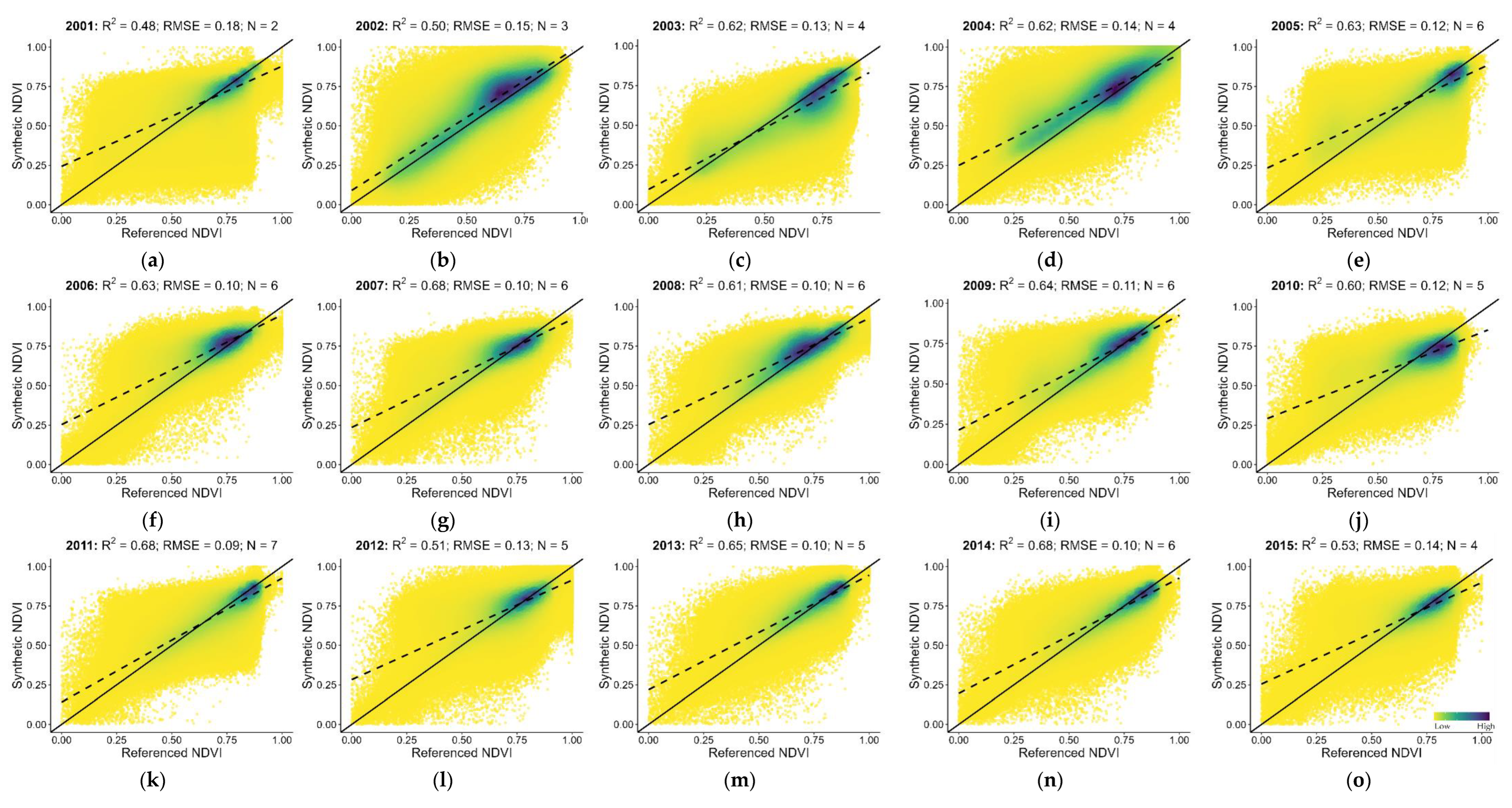
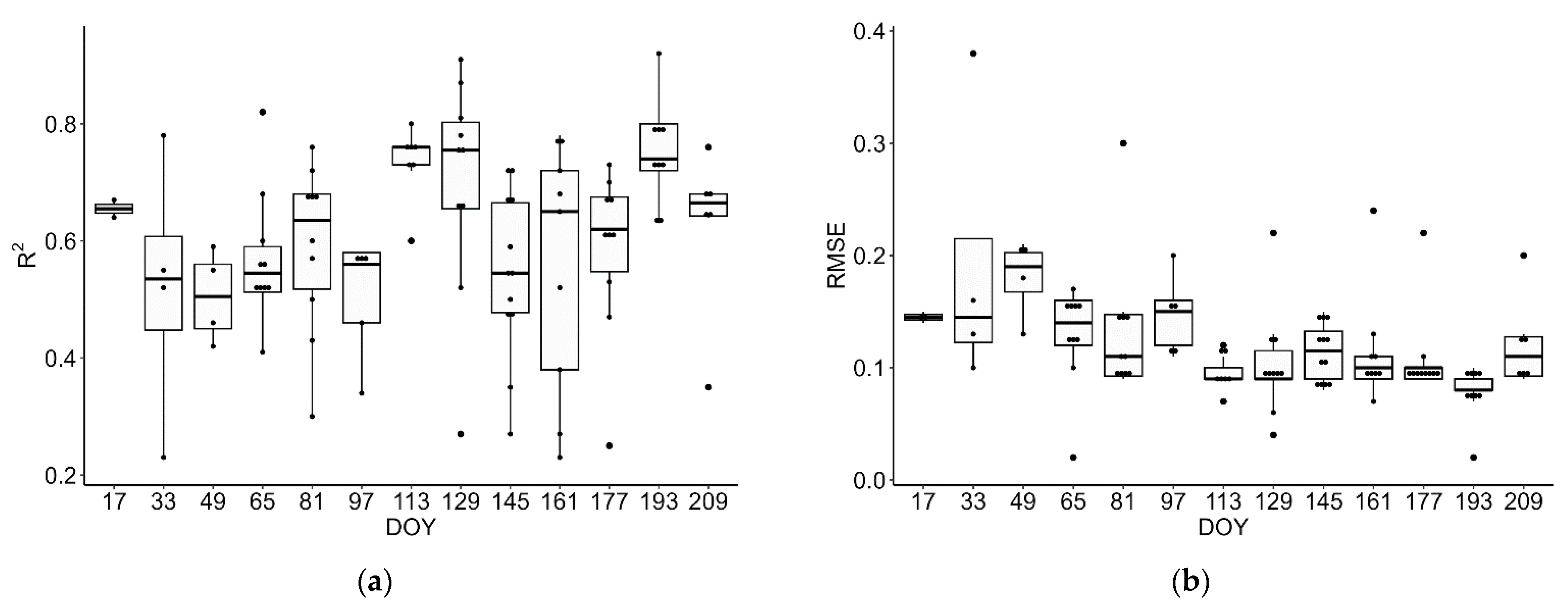
3.1. Validation of Synthetic Remote Sensing Time Series from 2001 to 2019

For nineteen years (i.e., from 2001 to 2019), the STARFM performed significantly for yearly synthetic output (having a p-value < 0.05); this rejected the H₀ of the linear regression model that there was no correlation between the synthetic and referenced NDVI (Figure 3a–s). After generating the yearly scatter plots, the synthetic products’ R² and RMSE values were analysed. Among all years, the highest accuracy and precision were obtained for 2016 and 2018, with an average R² of 0.75 and RMSE of 0.09. For 2005, 2006, 2007, 2009, 2011, 2013, 2014, 2017, and 2019, the R² values were higher than 0.60 and the RMSE values were lower than 0.12. In other years, such as 2003, 2004, 2008, and 2010, the R² and RMSE values lied within 0.60 to 0.62 and 0.10 to 0.14, respectively. However, the rest of the temporal period (i.e., 2001, 2002, 2012, and 2015) resulted in lower R² (<0.60) and RMSE (>0.13) values.

The results proved that the yearly accuracy assessment of the synthetic products is impacted by the total number of Landsat scenes (N) available every year (Figure 4a,b). A high positive (R = +0.83) and negative (R = −0.84) correlation was seen between the yearly quality (R²) and preciseness (RMSE) of the synthetic NDVI products with N, respectively. For example, 2011, 2016, and 2018 were the most accurate years (R² > 0.68 and RMSE = 0.09) with a total N of more than 7. Similarly, 2001 and 2002 had the least R² (< 0.50) and highest RMSE (> 0.15) with the fewest available Landsat scenes (N = 2/3) in both years. The overall accuracy of L-MOD13Q1 for nineteen years was R² of 0.62 and RMSE of 0.12, with an average of 5 N every year.

On comparing the yearly fusion results on a DOY basis, the DOYs 113, 129, and 193 had the highest average accuracy with an R² of more than 0.65 and a RMSE lesser than 0.10 (Figure 5a,b). The DOYs of 33 to 97 and 145 to 177, with low R² (<0.60) and high RMSE (>0.11), were obtained.

3.2. Comparative Analysis between Crop Yield Accuracy of MOD13Q1 and L-MOD13Q1 Using the Light Use Efficiency Model in 2019

Figure 6a–c displayed the crop yield accuracies between the modelled and referenced crop yields of WW and OSR obtained with different satellite products using the LUE model in 2019. The figures show that the fused product (L-MOD13Q1) obtained a higher R² (0.81) and a lower RMSE (3.91 dt/ha) than the non-fused product (MOD13Q1: R² = 0.70 and RMSE = 4.77 dt/ha) for both WW and OSR. Analysing the ME of both products with LUE, the L-MOD13Q1 resulted in a lower ME (3.04 dt/ha) than the MOD13Q1 (3.50 dt/ha) (Figure 6c).

3.3. Statistical Analysis between Reference and Modelled Crop Yields of WW and OSR from 2001 to 2019 Using the Light Use Efficiency Model

For both WW and OSR, the LUE model performed significantly for every year (having a p-value < 0.05); this rejected the H₀ of the linear regression model that there was no correlation between the referenced and modelled crop yield from 2001 to 2019 (Figure A3a–s and Figure A4a–s). After generating the scatter plots, all crop yield products’ R², RMSE, and ME values were analysed. For both WW and OSR, the years 2007 through 2018 and 2019 were the most accurate years where the estimated crop yield resulted in high R² values (>0.79). However, both 2018 and 2019 for WW resulted in higher RMSE (4.74 and 4.98 dt/ha) and ME (3.46 and 3.71 dt/ha) values, respectively (Figure A3). The remaining years for WW showed a similar trend in R² (>0.65), RMSE (<4.50 dt/ha), and ME (<3.60 dt/ha) values, with the exceptions of 2001 and 2013, which had RMSE values more than 5.40 dt/ha and ME values more than 4.30 dt/ha. Similarly, for OSR, the RMSE values for 2001, 2005, and 2012 resulted in higher RMSE (>3.22 dt/ha) and ME (>2.47 dt/ha) (Figure A4). A mostly, similar trend in R² values was observed in the OSR, with values ranging from 0.63 to 0.80. The overall accuracies of both WW and OSR for 19 years were recorded as R² of 0.79 and 0.86 and RMSE of 4.51 dt/ha and 2.47 dt/ha, respectively (Figure 7a,b). Negative correlations were seen between the regional mean elevations and the modelled yields of WW (−0.30) and OSR (−0.38), respectively (Figure 8a,b).

3.4. Sensitivity Analysis

The sensitivity analysis compared the model’s performance by excluding the effect of climate stress factors from 2001 to 2019 for both WW and OSR in Bavaria. The LUE-modelled yield showed a higher correlation with the referenced yield when the climate stress factors were included, and vice versa. The model showed higher R² and lower RMSE values when compared with the yield values obtained during the sensitivity analysis (Figure 9a,b). The overall accuracies obtained during the sensitivity analysis of both WW and OSR for 19 years were recorded as R² of 0.68 and 0.78 and RMSE of 5.88 dt/ha and 3.41 dt/ha, respectively (Figure 9c,d).

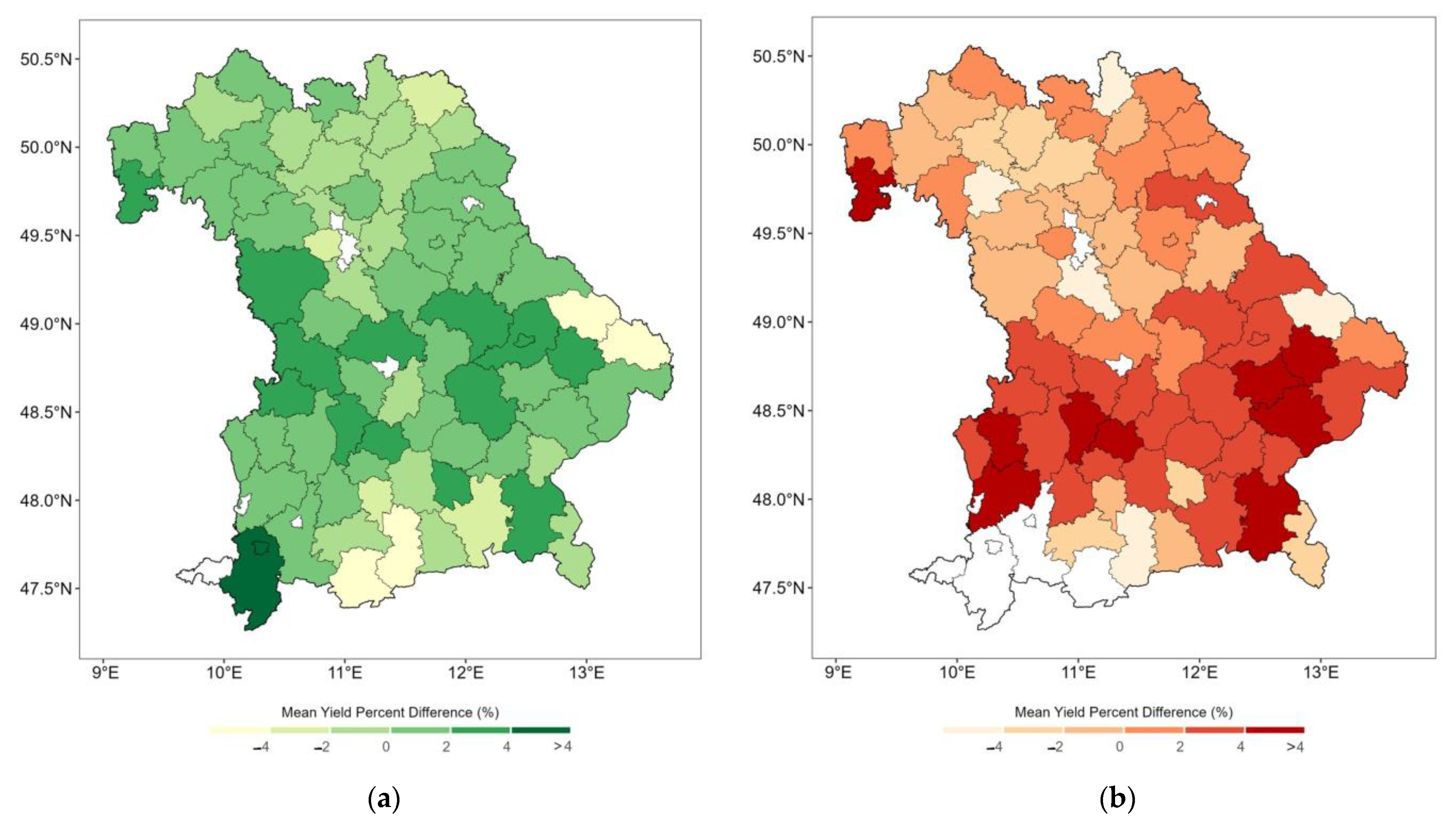
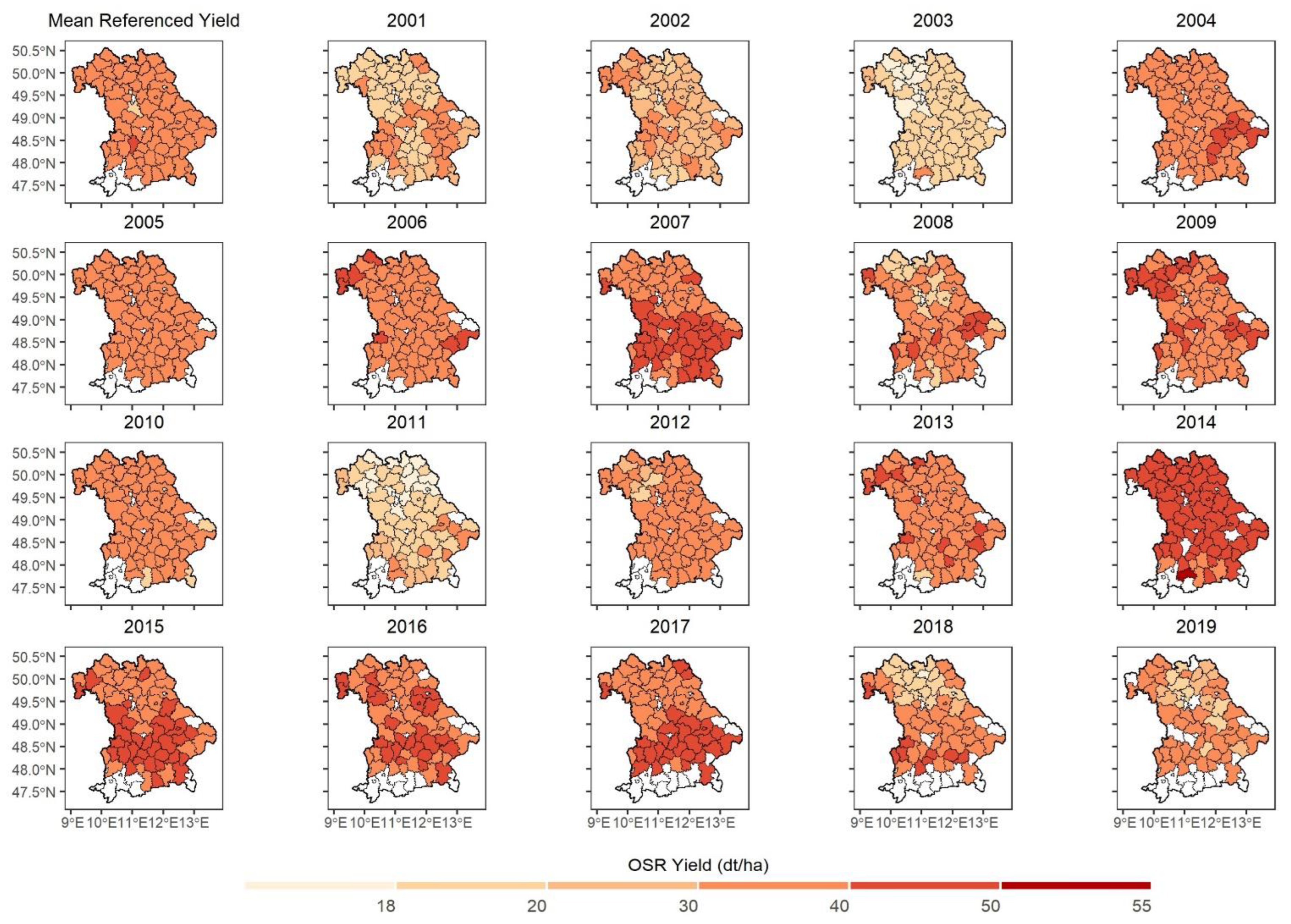
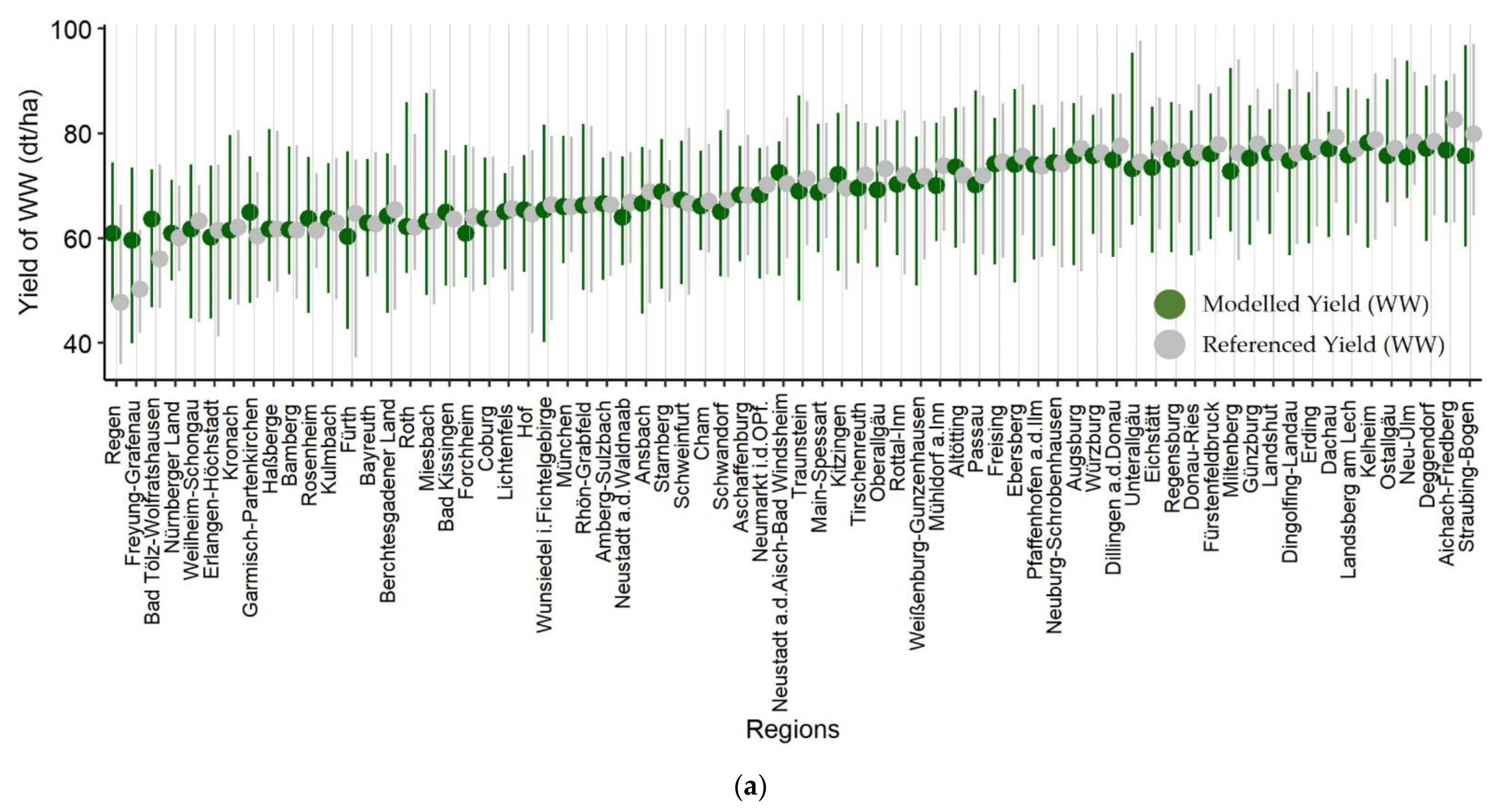
3.5. Statistical Analysis between Reference and Modelled Crop Yields of WW and OSR from 2001 to 2019 Using the Light Use Efficiency Model at Regional Level

On comparing the long-term crop yield at the regional level, the yearly spatial change from the mean referenced and modelled yield was displayed for both WW and OSR (Figure 10 and Figure 11). For WW, most of the regional yield lied between 65 and 80 dt/ha (Figure 10). Districts such as, Regen, Freyung-Grafenau, Bad Tölz-Wolfratshausen, and Garmisch-Partenkirchen, the average percent difference was calculated as −25.10% (LUE: ~75 dt/ha), −18.68% (~60 dt/ha), −8.08% (~62 dt/ha), and −5.58% (~65 dt/ha), which showed that the model highly overestimated the crop yield values as compared to the referenced yield (Figure 12a and Figure A5a). The positive yield percent difference (where the model underestimated the crop yield) between 0 and 4% had an accuracy greater than 0.80 as compared to the negative yield percent difference between −4 and 0% with an accuracy less than 0.70 (Figure 13). Similarly, the model underestimated the crop yield of Oberallgäu, Miltenberg, Deggendorf, and Dachau with 4.65% (~78 dt/ha), 3.91% (~68 dt/ha), 3.30% (~75 dt/ha) and 3.15% (~78 dt/ha), respectively. Similarly for OSR, the model overestimated the yield for Aichach-Friedberg, Deggendorf, Dingolfing-Lindau, Traunstein, Unterallgäu, Dachau, Rottal-Inn, Miltenberg and Günzberg with 7.13% (LUE: ~38 dt/ha), 5.12% (~39 dt/ha), 4.91% (~37 dt/ha), 4.80% (~35 dt/ha), 4.53% (~36 dt/ha), 4.36% (~38 dt/ha), 4.25% (~35 dt/ha), 4.24% (~37 dt/ha) and 4.06% (~34 dt/ha), respectively (Figure 12b and Figure A5b). However, unlike WW, both the over- and underestimation of OSR yield values resulted in a similar increase and decrease in accuracy (Figure 13).

3.6. Correlation Analysis between the Accuracy Assessments of the Input Synthetic Products and the Crop Yield Modelling

The bar and scatter plots compared and linked the yearly accuracies of the input synthetic time series with the crop yield modelling for WW and OSR from 2001 to 2019, respectively (Figure 14 and Figure 15). For WW, the correlation coefficient showed a higher positive correlation of 0.81 between the R² of synthetic accuracy and the modelled yield accuracy (Figure 15a). Except 2015 (yield R²: 0.77, synthetic R²: 0.53) and 2013 (yield R²: 0.71, synthetic R²: 0.65), where the fusion accuracies were negatively correlated with crop yield accuracy (Figure 14a). Similarly, for OSR, the correlation coefficient was found to be 0.77 (Figure 15b). For 2001 and 2002, the fusion accuracy was lower (R² < 0.50); however, the crop yield accuracy for the same years resulted in an R² of more than 0.65 (Figure 14b).

3.7. Visualisation of the Modelled Crop Biomass and the NDVI of Different Years at a Field Level

The side-by-side spatial visualisation of the input synthetic NDVI product (DOY 169: 18 June) and the WW-modelled biomass for selected years (2005, 2013, and 2019) is shown in Figure 16, respectively. For every year, the spatial trend of crop biomass and NDVI in every field was seen differently. Likewise, NDVI values were rising from 2005 to 2019 from 0.4 to 0.8, and crop biomass had been observed rising from less than 550 g/m² in 2005 to more than 850 g/m² in 2019. In most of the fields, the crop biomass was dependent on the higher NDVI values. The NDVI values higher than 0.8 impacted higher crop biomass of more than 850 g/m² in almost every year. In 2005, the average field crop biomass resulted in less than 650 g/m²; however, in 2019, the crop biomass resulted in more than 650 g/m².

4. Discussion

4.1. Quality Assessment of Synthetic Remote Sensing Time Series from 2001 to 2019

The present study investigates the potential of the STARFM over the Bavarian state of Germany to generate the synthetic NDVI time series from 2001 to 2019 by selecting the best-performing high (Landsat) and low (MODIS) pair obtained for the agricultural class from the previous literature. Many studies prefer using ESTARFM (Enhanced STARFM) for better fusion accuracy [80,81]; however, some studies found STARFM performing significantly better than ESTARFM [82,83]. Simple in its design, faster to implement, and capable of fusing the entire state of Bavaria (which covers almost one-fifth of the area of Germany) for two decades, the study finds STARFM to be more advantageous over ESTARFM. ESTARM was complex, time-consuming, and computationally expensive for covering extensive data for extended periods [84,85]. One of the strengths of ESTARFM is that it incorporates additional information, such as a land-cover map, to improve the accuracy of the fusion [80]. The study incorporates Bavaria’s accurate and updated land cover map into the STARFM to balance its input requirements with the ESTARFM. It provided homogeneity to the STARFM and increased its fusion accuracy (as discussed briefly in our previous study [59]).

In our previous study, we found that L-MOD13Q1 (30 m, 16 days) (R² = 0.62 and RMSE = 0.11) was suitable for the application of agricultural monitoring due to its fast and easy processing with lesser storage requirements [59]. Moreover, the present study focuses on two decades (2001 to 2019); therefore, the paper generates and validates a Landsat-based synthetic NDVI time series (L-MOD13Q1) due to its continuous availability since 1982 with a maximum resolution of 30 m. As NDVI is among the most effective and widely used vegetation indices, many spatiotemporal fusion-based studies have used it as their primary input [5,30,36,37]. However, many spatiotemporal fusion algorithms are based on reflectance fusion, which requires more processing time and storage than NDVI (or one-band blending) fusion [86,87]. Having high computation power with fewer storage problems for the long-term time series of 2001 to 2019 for complete Bavaria (70,550 km²), the research uses the strategy “index-then-blend” (IB), which generates the NDVI from Landsat and MOD13Q1 before they are blended for fusion [88]. The IB strategy is used in multiple works of the literature with highly accurate and precise fusion outputs [17,59,88].

The analysis found that the accuracies of the fusion products are dependent on the available number of Landsat scenes per year (N) [59], such that the higher N, the higher the fusion accuracy of the synthetic NDVI product in a respective year. For instance, the positive R (+0.75) shows the positive correlation between R² of yearly synthetic NDVIs and N (representing the higher quality of the fused product), and the negative R (−0.73) shows the negative correlation between RMSEs and N (representing the higher precision). However, as the research made use of Landsat 8 Operational Land Imager (OLI) (from 2013 to 2019) and Landsat 5 Thematic Mapper (TM) (from 2001 to 2013), it was found that Landsat OLI-based fusion with MOD13Q1 resulted in higher accuracy as compared to Landsat TM [89]. For example, the years 2001, 2002, 2004, 2005, and 2012 (using Landsat 5 and 7) have a lower R² (<0.60) and a higher RMSE (>0.12) than the remaining years (using Landsat 8). The reason could be that Landsat 8 has improved upon the quality of Landsat 5 and 7, offering improved data accuracy. Moreover, the accuracy of the year 2012 is affected due to the gaps generated by the scan line corrector (SLC) failure in Landsat 7.

On comparing the fusing results on a DOY basis, the study finds that the few cloud-free DOYs could create large gaps between the available Landsat scenes that might affect the accuracy of the fusion product [17,59]. For example, the DOYs 33 to 97 (N = ~6) result in a low R² (0.54) and a high RMSE (0.16) as compared to the DOYs 113 to 193 (N = ~8), which have a high R² (0.64) and a low RMSE (0.10).

4.2. Impact of Synthetic Time Series on Crop Yield Modelling

The objective of the present study is to generate and validate the long-term crop yield time series using the semi-empiric LUE model, which has proven to be more reliable, precise, and simple in the previous literature [17,42]. The present study validates the crop yield results of WW and OSR obtained by inputting the synthetic NDVI and climate elements to the LUE model at a regional scale in Bavaria from 2001 to 2019. However, before generating the long-term time series using the synthetic NDVI product, the study finds the potential of fused (L-MOD13Q1) in crop yield prediction by comparing its accuracies with the non-fused (MOD13Q1) product in 2019. The study obtains higher crop yield accuracy with the L-MOD13Q1 (R² = 0.81 and RMSE = 3.91 dt/ha) than the MOD13Q1 (R² = 0.70 and RMSE = 4.77 dt/ha) irrespective of the crop type (Figure 6a,b). It proves the importance of high-resolution synthetic data for accurate modelling of crop yields.

After generating the long-term crop yield time series, the research finds the significant yearly performance of the model for both WW and OSR; however, some years obtained higher accuracy than the others. For example, 2007, 2018, and 2019 are the most accurate years, with R² values of more than 0.79 for both crop types. However, the RMSEs of both 2018 and 2019 are relatively higher (>4.74 dt/ha) than in the other years. Similarly, 2011 and 2016, with a higher number of N (~6), result in lower crop yield accuracy than 2007, 2008, and 2011 (N = ~8). This might be due to the impact of climate variables inputted into the LUE model (discussed briefly in Section 4.3).

The study discusses briefly how the quality of the input data fusion product impacts the accuracy of the CGM. For example, due to the low quality of synthetic NDVI products in 2001, 2002, and 2012, which might impact the accuracy of the input FPAR products generated, the yield prediction accuracy of both WW and OSR is low. The analysis tries to prove that even though synthetic time series would be the preferable solution to input a CGM for yield prediction when the quality of the combined fusion product is low, it could negatively affect the crop yield estimation. In relevance to the above point, high positive correlations have been seen when the accuracies of the synthetic NDVI time series are plotted with the accuracies of modelled crop yield from 2001 to 2019 for WW (R = 0.81) and OSR (0.77). For example, the quality of the NDVI time series for the years 2016 and 2018 is higher with R² (>0.73), and the crop yield accuracies are also higher with R² of 0.83 (WW)/0.81 (OSR), 0.85/0.83, respectively (Figure 3p,r). Similarly, the striped data collected from Landsat 7 in 2012 has deteriorated the quality of the synthetic NDVI product (R² = 0.51; RMSE = 0.13), which further negatively affected the crop yield estimations for WW (R² = 0.62; RMSE = 5.40 dt/ha) and OSR (R² = 0.49; RMSE = 4.13 dt/ha) (Figure 3l). Moreover, the Landsat images were available at different times of the year. This has an impact on the prediction accuracy of both crops. For example, the WW yield results are more accurate than the OSR because the synthetic data in late spring and early summer (DOYs 113 to 193) is usually more precise.

The study compares the long-term crop yield time series by calculating the average percent change from the referenced and modelled yields for both crop types. Previous studies found that the elevation plays a significant role in impacting the regional crop yield [90,91]. Most of the studies found lower crop productivity at higher elevations due to complex topography, different climates, and management practices [92,93]. Moreover, the cropping intensity at lower elevations is higher as compared to the higher elevations. The survey finds negative correlations between the mean regional elevations and the crop yields of WW (−0.30) and OSR (−0.38). The model is precarious in specific regions, especially the districts at higher elevations in the south (Bavarian Alps) and east (Bavarian Forest and Fichtel Mountains) of Bavaria for both WW and OSR. In regions such as Regen, Freyung-Grafenau, Bad Tölz-Wolfratshausen, and Garmisch-Partenkirchen, the model highly overestimates the crop yield, and for regions such as Oberallgäu, Miltenberg, Deggendorf, and Dachau, it underestimates the yield as compared to the referenced yield for WW. This overestimation of WW yield values has resulted in a decrease in accuracy. The model shows yearly stability in predicting crop yields of WW between 65 and 80 dt/ha for most of the regions. The positive yield percent change (where the model underestimated the crop yield) between 0 and 4% had higher accuracy (R² > 0.80) as compared to the percent change between −4 and 0% (R² < 0.70). For 48 of the 71 total districts, the model performs relatively well, with a percent change between –2% and +2%. However, unlike WW, both the over- and underestimation-yield values have resulted in a similar increase and decrease in the accuracy of OSR. The positive and negative yield percent change (where the model under- and over-estimates the crop yield, respectively) between 0 and +/−4% had an accuracy of more than 0.80. For OSR, the model overestimates the yield for Aichach-Friedberg, Deggendorf, Dingolfing-Lindau, Traunstein, Unterallgäu, Dachau, Rottal-Inn, Miltenberg, and Günzberg and underestimates the yield for Roth, Regen, Kronach, Kitzingen, and Bad Tölz-Wolfratshausen. However, for the 27 districts with OSR, the model performs steadily. Interestingly, the regions where the model’s performance went unstable were primarily located in the southern alps, except for Regen, Freyung-Grafenau, Kitzingen, Roth, and Miltenberg. The reason could be the instability of the model at higher elevations or the bad quality of the synthetic NDVI products in specific districts. The quality of the synthetic NDVI product might vary for these regions as the districts have no horizontal or vertical overlay of Landsat scenes within the path row, limiting their coverage frequency.

4.3. Sensitivity Analysis

Besides the impact of data fusion, climate variables play an essential role in affecting the accuracy of crop yield predictions [31,94,95]. To analyse the impact of climate elements, the study performs sensitivity analysis, where the LUE model calculates the crop yields of WW and OSR without including the climate stress factors from 2001 to 2019. As the referenced yield is already influenced by the climate, the results of the study show that the accuracy of crop yield predictions worsens with the exclusion of climate variables, with a lower R² (0.68 (WW)/0.74 (OSR)) and a higher RMSE (5.88/3.41 dt/ha). However, an increase in R² (0.79/0.86) and decrease in RMSE (4.51/2.57 dt/ha) have been seen when the climate effect is included in the model. As the relationship between climate and crop yield undergoes significant shifts, it might be the reason that some years (2011 and 2016) with higher N (8) obtained lower crop yield accuracy than years (2007, 2018 and 2019) with comparably lower N (6). Moreover, our previous study, which made use of the machine learning approach with the LUE model, identified the impact of every individual climate element used in crop yield predictions [31].

Furthermore, many studies stated that the availability of coarse climate data negatively affected yield prediction accuracy. In a previous study, the coarse spatial resolution of climate data (ECMWF: ~80 km) used to estimate the biomass resulted in low R² and high RMSE using CGMs by inputting coarse synthetic NDVI products [17,42]. However, while inputting high spatial resolution NDVI products, the low impact of the high spatial resolution of climate elements is observed. The present study inputs high spatial resolution climate data time series (2 km, daily) to the LUE model, resulting in stable yearly accuracies from 2001 to 2019. Notably, selecting climate thresholds according to the geographical location and crop types is essential in achieving high crop yield accuracy [96,97,98]. Different climate thresholds are used for WW and OSR, resulting in accurate and stable yield predictions in Bavaria during the study period.

4.4. Validation at the District Level

The crop yield validation for the more extended time series of 2001 to 2019 is performed using the LfStat crop yield data (used for validation at a 95% confidence interval) for WW and OSR provided by the Bavarian State Office of Statistics. As the validation data set is provided at a regional scale, pixel-based yield information is converted for both crop types to the regional level. However, transferring the field-based information to the district level could result in some uncertainties in the validation process. For example, in some regions of southern Bavaria (Bad Tölz-Wolfratshausen, Garmisch-Partenkirchen, Traunstein, Unterallgäu, and Oberallgäu), where the model’s performance is volatile, this might be due to the uncertainty occurring while transferring the pixel-level information to the district level. The availability of fewer fields of WW and OSR in those regions might be the reason for the model’s instability, as the validation data recorded high yield values for the same districts. Therefore, future work should aim to validate crop yield results at the field level, which could help achieve more precise results. Additionally, the availability of field data for FPAR, an important input to the LUE model, would help to validate the FPAR product generated using the NDVI time series.

5. Conclusions

The present study investigates the relationship of spatiotemporal fusion modelling using STRAFM on crop yield prediction for winter wheat (WW) and oil-seed rape (OSR) using a semi-empirical light use efficiency (LUE) model for Bavaria, Germany, from 2001 to 2019. The research paper concludes the findings as follows:

(i)

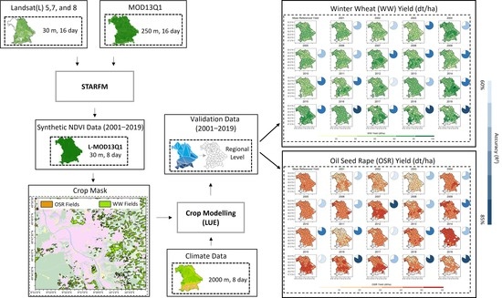
To find the potential of STARFM for long-term time series, the paper generates and validates a synthetic normalised difference vegetation index (NDVI) time series blending the high spatial resolution (30 m, 16 days) of Landsat 5 Thematic Mapper (TM) (2001 to 2012), Landsat 7 Enhanced Thematic Mapper Plus (ETM+) (2012), and Landsat 8 Operational Land Imager (OLI) (2013 to 2019) with the coarse resolution of MOD13Q1 (250 m, 16 days) from 2001 to 2019. Overall, the average accuracy of data fusion for nineteen years has an R² of 0.66 and an RMSE of 0.11. The accuracy of data fusion is found to be dependent on the number of Landsat scenes available per year (N). The higher the N, the more accurate is the synthetic NDVI time series per year.

(ii)

To investigate the stability and precision of the LUE model in crop yield prediction, the paper inputs the synthetic NDVI time series and climate elements to the crop model to estimate and validate yearly crop yields for WW and OSR from 2001 to 2019. The validation of crop yield at regional scale results in an average R² of 0.79 (WW)/0.86 (OSR) and an RMSE of 4.51 dt/ha/2.46 dt/ha, respectively.

(iii)

Identifying the impact of the input data fusion product on the accuracy assessment of the LUE model, high positive correlations are seen when the accuracies of the synthetic NDVI time series are plotted with the accuracies of modelled crop yield from 2001 to 2019 for WW (R = 0.81) and OSR (0.77).

The present study recommends validating crop yields at the field scale, as transferring the pixel-based information to the district level could cause uncertainties in the validation process. The accurate crop yield predictions from the analysis for WW and OSR could be further used for the application of biodiversity, where the impact of land use diversity on crop yields could be estimated. The ease of using spatiotemporal modelling with crop growth models would not be limited to Bavaria. The study’s methodology could also be tested by coupling machine/deep learning (ML/DL) approaches with CGMs, which might help to include more climate elements to achieve more precise results. Lastly, the study’s two decades of accurate yield estimations could strengthen trust in the decision(/policy) making to achieve sustainability in agriculture.

References

1. Mueller, N.D.; Gerber, J.S.; Johnston, M.; Ray, D.K.; Ramankutty, N.; Foley, J.A. Closing yield gaps through nutrient and water management. Nature 2012, 490, 254–257. [Google Scholar] [CrossRef] [PubMed]
2. Bian, C.; Shi, H.; Wu, S.; Zhang, K.; Wei, M.; Zhao, Y.; Sun, Y.; Zhuang, H.; Zhang, X.; Chen, S. Prediction of Field-Scale Wheat Yield Using Machine Learning Method and Multi-Spectral UAV Data. Remote Sens. 2022, 14, 1474. [Google Scholar] [CrossRef]
3. Fritz, S.; See, L.; Bayas, J.C.L.; Waldner, F.; Jacques, D.; Becker-Reshef, I.; Whitcraft, A.; Baruth, B.; Bonifacio, R.; Crutchfield, J. A comparison of global agricultural monitoring systems and current gaps. Agric. Syst. 2019, 168, 258–272. [Google Scholar] [CrossRef]
4. Ziliani, M.G.; Altaf, M.U.; Aragon, B.; Houborg, R.; Franz, T.E.; Lu, Y.; Sheffield, J.; Hoteit, I.; McCabe, M.F. Early season prediction of within-field crop yield variability by assimilating CubeSat data into a crop model. Agric. For. Meteorol. 2022, 313, 108736. [Google Scholar] [CrossRef]
5. Eurostat, Waste Statistics- Electrical and Electronic Equipment. 2019. Available online: https://ec.europa.eu/eurostat/statistics-explained/index.php (accessed on 7 August 2020).
6. Alarcón-Segura, V.; Grass, I.; Breustedt, G.; Rohlfs, M.; Tscharntke, T. Strip intercropping of wheat and oilseed rape enhances biodiversity and biological pest control in a conventionally managed farm scenario. J. Appl. Ecol. 2022, 59, 1513–1523. [Google Scholar] [CrossRef]
7. Macholdt, J.; Honermeier, B. Yield stability in winter wheat production: A survey on German farmers’ and advisors’ views. Agronomy 2017, 7, 45. [Google Scholar] [CrossRef] [Green Version]
8. Lutter, S.; Giljum, S.; Gözet, B.; Wieland, H.; Manstein, C. The Use of Natural Resources: Report for Germany 2018; Bundesamt, U., Ed.; Federal Environment Agency: Dessau, Germany, 2018.
9. UFOP. Union zur Förderung von oel-und Proteinpflanzen E.V. Available online: https://www.ufop.de/ (accessed on 13 July 2021).
10. Ali, A.M.; Abouelghar, M.A.; Belal, A.-A.; Saleh, N.; Younes, M.; Selim, A.; Emam, M.E.; Elwesemy, A.; Kucher, D.E.; Magignan, S. Crop Yield Prediction Using Multi Sensors Remote Sensing. Egypt. J. Remote Sens. Space Sci. 2022, 25, 711–716. [Google Scholar]
11. Justice, C.; Townshend, J.; Vermote, E.; Masuoka, E.; Wolfe, R.; Saleous, N.; Roy, D.; Morisette, J. An overview of MODIS Land data processing and product status. Remote Sens. Environ. 2002, 83, 3–15. [Google Scholar] [CrossRef]
12. Ahmad, I.; Ghafoor, A.; Bhatti, M.I.; Akhtar, I.-u.H.; Ibrahim, M. Satellite remote sensing and GIS-based crops forecasting & estimation system in Pakistan. Crop Monit. Improv. Food Secur. 2014, 28, 95–109. [Google Scholar]
13. Karila, K.; Nevalainen, O.; Krooks, A.; Karjalainen, M.; Kaasalainen, S. Monitoring changes in rice cultivated area from SAR and optical satellite images in Ben Tre and Tra Vinh Provinces in Mekong Delta, Vietnam. Remote Sens. 2014, 6, 4090–4108. [Google Scholar] [CrossRef] [Green Version]
14. Friedl, M.A.; Sulla-Menashe, D.; Tan, B.; Schneider, A.; Ramankutty, N.; Sibley, A.; Huang, X. MODIS Collection 5 global land cover: Algorithm refinements and characterization of new datasets. Remote Sens. Environ. 2010, 114, 168–182. [Google Scholar] [CrossRef]
15. Lobell, D.B. The use of satellite data for crop yield gap analysis. Field Crops Res. 2013, 143, 56–64. [Google Scholar] [CrossRef] [Green Version]
16. Ogutu, B.O.; Dash, J. An algorithm to derive the fraction of photosynthetically active radiation absorbed by photosynthetic elements of the canopy (FAPAR ps) from eddy covariance flux tower data. New Phytol. 2013, 197, 511–523. [Google Scholar] [CrossRef] [PubMed]
17. Dhillon, M.S.; Dahms, T.; Kuebert-Flock, C.; Borg, E.; Conrad, C.; Ullmann, T. Modelling Crop Biomass from Synthetic Remote Sensing Time Series: Example for the DEMMIN Test Site, Germany. Remote Sens. 2020, 12, 1819. [Google Scholar] [CrossRef]
18. Wulder, M.A.; Loveland, T.R.; Roy, D.P.; Crawford, C.J.; Masek, J.G.; Woodcock, C.E.; Allen, R.G.; Anderson, M.C.; Belward, A.S.; Cohen, W.B. Current status of Landsat program, science, and applications. Remote Sens. Environ. 2019, 225, 127–147. [Google Scholar] [CrossRef]
19. Wulder, M.A.; White, J.C.; Loveland, T.R.; Woodcock, C.E.; Belward, A.S.; Cohen, W.B.; Fosnight, E.A.; Shaw, J.; Masek, J.G.; Roy, D.P. The global Landsat archive: Status, consolidation, and direction. Remote Sens. Environ. 2016, 185, 271–283. [Google Scholar] [CrossRef] [Green Version]
20. Wulder, M.A.; Masek, J.G.; Cohen, W.B.; Loveland, T.R.; Woodcock, C.E. Opening the archive: How free data has enabled the science and monitoring promise of Landsat. Remote Sens. Environ. 2012, 122, 2–10. [Google Scholar] [CrossRef]
21. Souza, E.; Bazzi, C.; Khosla, R.; Uribe-Opazo, M.; Reich, R.M. Interpolation type and data computation of crop yield maps is important for precision crop production. J. Plant Nutr. 2016, 39, 531–538. [Google Scholar] [CrossRef]
22. Mariano, C.; Monica, B. A random forest-based algorithm for data-intensive spatial interpolation in crop yield mapping. Comput. Electron. Agric. 2021, 184, 106094. [Google Scholar] [CrossRef]
23. Nemecek, T.; Weiler, K.; Plassmann, K.; Schnetzer, J.; Gaillard, G.; Jefferies, D.; García–Suárez, T.; King, H.; i Canals, L.M. Estimation of the variability in global warming potential of worldwide crop production using a modular extrapolation approach. J. Clean. Prod. 2012, 31, 106–117. [Google Scholar] [CrossRef]
24. Atamanyuk, I.; Kondratenko, Y.; Shebanin, V.; Sirenko, N.; Poltorak, A.; Baryshevska, I.; Atamaniuk, V. Forecasting of cereal crop harvest on the basis of an extrapolation canonical model of a vector random sequence. CEUR Workshop Proc. 2019, II, 302–315. [Google Scholar]
25. Bolton, D.K.; Friedl, M.A. Forecasting crop yield using remotely sensed vegetation indices and crop phenology metrics. Agric. For. Meteorol. 2013, 173, 74–84. [Google Scholar] [CrossRef]
26. Johnson, M.D.; Hsieh, W.W.; Cannon, A.J.; Davidson, A.; Bédard, F. Crop yield forecasting on the Canadian Prairies by remotely sensed vegetation indices and machine learning methods. Agric. For. Meteorol. 2016, 218, 74–84. [Google Scholar] [CrossRef]
27. Ramesh, D.; Vardhan, B.V. Analysis of crop yield prediction using data mining techniques. Int. J. Res. Eng. Technol. 2015, 4, 47–473. [Google Scholar]
28. Mo, X.; Liu, S.; Lin, Z.; Xu, Y.; Xiang, Y.; McVicar, T. Prediction of crop yield, water consumption and water use efficiency with a SVAT-crop growth model using remotely sensed data on the North China Plain. Ecol. Model. 2005, 183, 301–322. [Google Scholar] [CrossRef]
29. Ghadge, R.; Kulkarni, J.; More, P.; Nene, S.; Priya, R. Prediction of crop yield using machine learning. Int. Res. J. Eng. Technol. (IRJET) 2018, 5, 2237–2239. [Google Scholar]
30. Van Klompenburg, T.; Kassahun, A.; Catal, C. Crop yield prediction using machine learning: A systematic literature review. Comput. Electron. Agric. 2020, 177, 105709. [Google Scholar] [CrossRef]
31. Dhillon, M.S.; Dahms, T.; Kuebert-Flock, C.; Rummler, T.; Arnault, J.; Stefan-Dewenter, I.; Ullmann, T. Integrating random forest and crop modeling improves the crop yield prediction of winter wheat and oil seed rape. Front. Remote Sens. 2023, 3, 109. [Google Scholar] [CrossRef]
32. Elavarasan, D.; Vincent, P.D. Crop yield prediction using deep reinforcement learning model for sustainable agrarian applications. IEEE Access 2020, 8, 86886–86901. [Google Scholar] [CrossRef]
33. Kuwata, K.; Shibasaki, R. Estimating crop yields with deep learning and remotely sensed data. In Proceedings of the 2015 IEEE International Geoscience and Remote Sensing Symposium (IGARSS), Milan, Italy, 26–31 July 2015; pp. 858–861. [Google Scholar]
34. Zhuo, W.; Fang, S.; Gao, X.; Wang, L.; Wu, D.; Fu, S.; Wu, Q.; Huang, J. Crop yield prediction using MODIS LAI, TIGGE weather forecasts and WOFOST model: A case study for winter wheat in Hebei, China during 2009–2013. Int. J. Appl. Earth Obs. Geoinf. 2022, 106, 102668. [Google Scholar] [CrossRef]
35. Kasampalis, D.A.; Alexandridis, T.K.; Deva, C.; Challinor, A.; Moshou, D.; Zalidis, G. Contribution of remote sensing on crop models: A review. J. Imaging 2018, 4, 52. [Google Scholar] [CrossRef] [Green Version]
36. Mirschel, W.; Schultz, A.; Wenkel, K.O.; Wieland, R.; Poluektov, R.A. Crop growth modelling on different spatial scales—A wide spectrum of approaches. Arch. Agron. Soil Sci. 2004, 50, 329–343. [Google Scholar] [CrossRef]
37. Murthy, V.R.K. Crop growth modeling and its applications in agricultural meteorology. Satell. Remote Sens. GIS Appl. Agric. Meteorol. 2004, 235, 235–261. [Google Scholar]
38. Iqbal, M.A.; Shen, Y.; Stricevic, R.; Pei, H.; Sun, H.; Amiri, E.; Penas, A.; del Rio, S. Evaluation of the FAO AquaCrop model for winter wheat on the North China Plain under deficit irrigation from field experiment to regional yield simulation. Agric. Water Manag. 2014, 135, 61–72. [Google Scholar] [CrossRef]
39. Van Dam, J.C.; Huygen, J.; Wesseling, J.; Feddes, R.; Kabat, P.; Van Walsum, P.; Groenendijk, P.; Van Diepen, C. Theory of SWAP Version 2.0. In Simulation of Water Flow, Solute Transport and Plant Growth in the Soil-Water-Atmosphere-Plant Environment; DLO Winand Staring Centre: Wageningen, The Netherlands, 1997. [Google Scholar]
40. Wang, E.; Robertson, M.; Hammer, G.; Carberry, P.S.; Holzworth, D.; Meinke, H.; Chapman, S.; Hargreaves, J.; Huth, N.; McLean, G. Development of a generic crop model template in the cropping system model APSIM. Eur. J. Agron. 2002, 18, 121–140. [Google Scholar] [CrossRef]
41. Spitters, C.; Van Keulen, H.; Van Kraalingen, D. A simple and universal crop growth simulator: SUCROS87. In Simulation and Systems Management in Crop Protection; Pudoc: Wageningen, The Netherlands, 1989; pp. 147–181. [Google Scholar]
42. Shi, Z.; Ruecker, G.R.; Mueller, M.; Conrad, C.; Ibragimov, N.; Lamers, J.; Martius, C.; Strunz, G.; Dech, S.; Vlek, P.L.G. Modeling of cotton yields in the amu darya river floodplains of Uzbekistan integrating multitemporal remote sensing and minimum field data. Agron. J. 2007, 99, 1317–1326. [Google Scholar] [CrossRef]
43. Van Diepen, C.A.v.; Wolf, J.; Van Keulen, H.; Rappoldt, C. WOFOST: A simulation model of crop production. Soil Use Manag. 1989, 5, 16–24. [Google Scholar] [CrossRef]
44. Potter, C.S.; Randerson, J.T.; Field, C.B.; Matson, P.A.; Vitousek, P.M.; Mooney, H.A.; Klooster, S.A. Terrestrial ecosystem production: A process model based on global satellite and surface data. Glob. Biogeochem. Cycles 1993, 7, 811–841. [Google Scholar] [CrossRef]
45. Duchemin, B.; Maisongrande, P.; Boulet, G.; Benhadj, I. A simple algorithm for yield estimates: Evaluation for semi-arid irrigated winter wheat monitored with green leaf area index. Environ. Model. Softw. 2008, 23, 876–892. [Google Scholar] [CrossRef] [Green Version]
46. Schwalbert, R.A.; Amado, T.; Corassa, G.; Pott, L.P.; Prasad, P.V.; Ciampitti, I.A. Satellite-based soybean yield forecast: Integrating machine learning and weather data for improving crop yield prediction in southern Brazil. Agric. For. Meteorol. 2020, 284, 107886. [Google Scholar] [CrossRef]
47. Kern, A.; Barcza, Z.; Marjanović, H.; Árendás, T.; Fodor, N.; Bónis, P.; Bognár, P.; Lichtenberger, J. Statistical modelling of crop yield in Central Europe using climate data and remote sensing vegetation indices. Agric. For. Meteorol. 2018, 260, 300–320. [Google Scholar] [CrossRef]
48. Shammi, S.A.; Meng, Q. Use time series NDVI and EVI to develop dynamic crop growth metrics for yield modeling. Ecol. Indic. 2021, 121, 107124. [Google Scholar] [CrossRef]
49. Gevaert, C.M.; García-Haro, F.J. A comparison of STARFM and an unmixing-based algorithm for Landsat and MODIS data fusion. Remote Sens. Environ. 2015, 156, 34–44. [Google Scholar] [CrossRef]
50. Roy, D.P.; Ju, J.; Lewis, P.; Schaaf, C.; Gao, F.; Hansen, M.; Lindquist, E. Multi-temporal MODIS–Landsat data fusion for relative radiometric normalization, gap filling, and prediction of Landsat data. Remote Sens. Environ. 2008, 112, 3112–3130. [Google Scholar] [CrossRef]
51. Benabdelouahab, T.; Lebrini, Y.; Boudhar, A.; Hadria, R.; Htitiou, A.; Lionboui, H. Monitoring spatial variability and trends of wheat grain yield over the main cereal regions in Morocco: A remote-based tool for planning and adjusting policies. Geocarto Int. 2019, 36, 2303–2322. [Google Scholar] [CrossRef]
52. Htitiou, A.; Boudhar, A.; Lebrini, Y.; Hadria, R.; Lionboui, H.; Elmansouri, L.; Tychon, B.; Benabdelouahab, T. The performance of random forest classification based on phenological metrics derived from Sentinel-2 and Landsat 8 to map crop cover in an irrigated semi-arid region. Remote Sens. Earth Syst. Sci. 2019, 2, 208–224. [Google Scholar] [CrossRef]
53. Lebrini, Y.; Boudhar, A.; Htitiou, A.; Hadria, R.; Lionboui, H.; Bounoua, L.; Benabdelouahab, T. Remote monitoring of agricultural systems using NDVI time series and machine learning methods: A tool for an adaptive agricultural policy. Arab. J. Geosci. 2020, 13, 796. [Google Scholar] [CrossRef]
54. Gao, F.; Masek, J.; Schwaller, M.; Hall, F. On the blending of the Landsat and MODIS surface reflectance: Predicting daily Landsat surface reflectance. IEEE Trans. Geosci. Remote Sens. 2006, 44, 2207–2218. [Google Scholar]
55. Cui, J.; Zhang, X.; Luo, M. Combining Linear pixel unmixing and STARFM for spatiotemporal fusion of Gaofen-1 wide field of view imagery and MODIS imagery. Remote Sens. 2018, 10, 1047. [Google Scholar] [CrossRef] [Green Version]
56. Lee, M.H.; Cheon, E.J.; Eo, Y.D. Cloud Detection and Restoration of Landsat-8 using STARFM. Korean J. Remote Sens. 2019, 35, 861–871. [Google Scholar]
57. Xie, D.; Zhang, J.; Zhu, X.; Pan, Y.; Liu, H.; Yuan, Z.; Yun, Y. An improved STARFM with help of an unmixing-based method to generate high spatial and temporal resolution remote sensing data in complex heterogeneous regions. Sensors 2016, 16, 207. [Google Scholar] [CrossRef] [PubMed] [Green Version]
58. Zhu, L.; Radeloff, V.C.; Ives, A.R. Improving the mapping of crop types in the Midwestern US by fusing Landsat and MODIS satellite data. Int. J. Appl. Earth Obs. Geoinf. 2017, 58, 1–11. [Google Scholar]
59. Dhillon, M.S.; Dahms, T.; Kübert-Flock, C.; Steffan-Dewenter, I.; Zhang, J.; Ullmann, T. Spatiotemporal Fusion Modelling Using STARFM: Examples of Landsat 8 and Sentinel-2 NDVI in Bavaria. Remote Sens. 2022, 14, 677. [Google Scholar] [CrossRef]
60. Miller, J. Agriculture and Forestry in Bavaria: Facts and Figures 2002; Bayerisches Staatsministerium für Landwirtschaft und Forsten: München, Germany, 2002. [Google Scholar]
61. Roy, D.P.; Kovalskyy, V.; Zhang, H.; Vermote, E.F.; Yan, L.; Kumar, S.; Egorov, A. CFEDharacterization of Landsat-7 to Landsat-8 reflective wavelength and normalized difference vegetation index continuity. Remote Sens. Environ. 2016, 185, 57–70. [Google Scholar] [CrossRef] [Green Version]
62. Sulik, J.J.; Long, D.S. Spectral indices for yellow canola flowers. Int. J. Remote Sens. 2015, 36, 2751–2765. [Google Scholar] [CrossRef]
63. Zamani-Noor, N.; Feistkorn, D. Monitoring Growth Status of Winter Oilseed Rape by NDVI and NDYI Derived from UAV-Based Red–Green–Blue Imagery. Agronomy 2022, 12, 2212. [Google Scholar] [CrossRef]
64. Harfenmeister, K.; Itzerott, S.; Weltzien, C.; Spengler, D. Detecting phenological development of winter wheat and winter barley using time series of sentinel-1 and sentinel-2. Remote Sens. 2021, 13, 5036. [Google Scholar] [CrossRef]
65. Meier, U.; Bleiholder, H.; Buhr, L.; Feller, C.; Hack, H.; Heß, M.; Lancashire, P.D.; Schnock, U.; Stauß, R.; Van Den Boom, T. The BBCH system to coding the phenological growth stages of plants–history and publications. J. Kult. 2009, 61, 41–52. [Google Scholar]
66. Hersbach, H.; Bell, B.; Berrisford, P.; Hirahara, S.; Horányi, A.; Muñoz-Sabater, J.; Simmons, A. The ERA5 global reanalysis. Q. J. R. Meteorol. Soc. 2020, 146, 1999–2049. [Google Scholar] [CrossRef]
67. Gochis, D.; Barlage, M.; Dugger, A.; FitzGerald, K.; Karsten, L.; McAllister, M.; McCreight, J.; Mills, J.; RafieeiNasab, A.; Read, L. The WRF-Hydro modeling system technical description, (Version 5.0). NCAR Tech. Note 2018, 107. [Google Scholar] [CrossRef]
68. Skamarock, W.C.; Klemp, J.B.; Dudhia, J.; Gill, D.O.; Liu, Z.; Berner, J.; Wang, W.; Powers, J.G.; Duda, M.G.; Barker, D.M. A Description of the Advanced Research WRF Model Version 4; National Center for Atmospheric Research: Boulder, CO, USA, 2019; Volume 145, p. 145. [Google Scholar]
69. Arnault, J.; Rummler, T.; Baur, F.; Lerch, S.; Wagner, S.; Fersch, B.; Zhang, Z.; Kerandi, N.; Keil, C.; Kunstmann, H. Precipitation sensitivity to the uncertainty of terrestrial water flow in WRF-Hydro: An ensemble analysis for central Europe. J. Hydrometeorol. 2018, 19, 1007–1025. [Google Scholar] [CrossRef]
70. Rummler, T.; Arnault, J.; Gochis, D.; Kunstmann, H. Role of lateral terrestrial water flow on the regional water cycle in a complex terrain region: Investigation with a fully coupled model system. J. Geophys. Res. Atmos. 2019, 124, 507–529. [Google Scholar] [CrossRef]
71. Farr, T.G.; Rosen, P.A.; Caro, E.; Crippen, R.; Duren, R.; Hensley, S.; Kobrick, M.; Paller, M.; Rodriguez, E.; Roth, L. The shuttle radar topography mission. Rev. Geophys. 2007, 45. [Google Scholar] [CrossRef] [Green Version]
72. Monteith, J.L. Solar radiation and productivity in tropical ecosystems. J. Appl. Ecol. 1972, 9, 747–766. [Google Scholar] [CrossRef] [Green Version]
73. Monteith, J.L. Climate and the efficiency of crop production in Britain. Philos. Trans. R. Soc. Lond. B Biol. Sci. 1977, 281, 277–294. [Google Scholar]
74. Asrar, G.; Myneni, R.; Choudhury, B. Spatial heterogeneity in vegetation canopies and remote sensing of absorbed photosynthetically active radiation: A modeling study. Remote Sens. Environ. 1992, 41, 85–103. [Google Scholar] [CrossRef]
75. Single, W.V. Frost injury and the physiology of the wheat plant. J. Aust. Inst. Agric. Sci. 1985, 51, 128–134. [Google Scholar]
76. Habekotté, B. A model of the phenological development of winter oilseed rape (Brassica napus L.). Field Crops Res. 1997, 54, 127–136. [Google Scholar] [CrossRef]
77. Hodgson, A. Repeseed adaptation in Northern New South Wales. II.* Predicting plant development of Brassica campestris L. and Brassica napus L. and its implications for planting time, designed to avoid water deficit and frost. Aust. J. Agric. Res. 1978, 29, 711–726. [Google Scholar] [CrossRef]
78. Russell, G.; Wilson, G.W. An Agro-Pedo-Climatological Knowledge-Base of Wheat in Europe; Brussels (Belgium) EC/JRC: Brussels Belgium, 1994. [Google Scholar]
79. Djumaniyazova, Y.; Sommer, R.; Ibragimov, N.; Ruzimov, J.; Lamers, J.; Vlek, P. Simulating water use and N response of winter wheat in the irrigated floodplains of Northwest Uzbekistan. Field Crops Res. 2010, 116, 239–251. [Google Scholar] [CrossRef]
80. Zhu, X.; Chen, J.; Gao, F.; Chen, X.; Masek, J.G. An enhanced spatial and temporal adaptive reflectance fusion model for complex heterogeneous regions. Remote Sens. Environ. 2010, 114, 2610–2623. [Google Scholar] [CrossRef]
81. Tewes, A.; Thonfeld, F.; Schmidt, M.; Oomen, R.J.; Zhu, X.; Dubovyk, O.; Menz, G.; Schellberg, J. Using RapidEye and MODIS data fusion to monitor vegetation dynamics in semi-arid rangelands in South Africa. Remote Sens. 2015, 7, 6510–6534. [Google Scholar] [CrossRef] [Green Version]
82. Ghosh, R.; Gupta, P.K.; Tolpekin, V.; Srivastav, S. An enhanced spatiotemporal fusion method–Implications for coal fire monitoring using satellite imagery. Int. J. Appl. Earth Obs. Geoinf. 2020, 88, 102056. [Google Scholar] [CrossRef]
83. Xue, J.; Leung, Y.; Fung, T. A Bayesian data fusion approach to spatio-temporal fusion of remotely sensed images. Remote Sens. 2017, 9, 1310. [Google Scholar] [CrossRef] [Green Version]
84. Chen, B.; Huang, B.; Xu, B. Comparison of spatiotemporal fusion models: A review. Remote Sens. 2015, 7, 1798–1835. [Google Scholar] [CrossRef] [Green Version]
85. Guo, Y.; Wang, C.; Lei, S.; Yang, J.; Zhao, Y. A framework of spatio-temporal fusion algorithm selection for landsat NDVI time series construction. ISPRS Int. J. Geo-Inf. 2020, 9, 665. [Google Scholar] [CrossRef]
86. Dong, T.; Liu, J.; Qian, B.; Zhao, T.; Jing, Q.; Geng, X.; Wang, J.; Huffman, T.; Shang, J. Estimating winter wheat biomass by assimilating leaf area index derived from fusion of Landsat-8 and MODIS data. Int. J. Appl. Earth Obs. Geoinf. 2016, 49, 63–74. [Google Scholar] [CrossRef]
87. Walker, J.J.; De Beurs, K.M.; Wynne, R.H.; Gao, F. Evaluation of Landsat and MODIS data fusion products for analysis of dryland forest phenology. Remote Sens. Environ. 2012, 117, 381–393. [Google Scholar] [CrossRef]
88. Chen, X.; Liu, M.; Zhu, X.; Chen, J.; Zhong, Y.; Cao, X. “Blend-then-Index” or “Index-then-Blend”: A theoretical analysis for generating high-resolution NDVI time series by STARFM. Photogramm. Eng. Remote Sens. 2018, 84, 65–73. [Google Scholar] [CrossRef]
89. Poursanidis, D.; Chrysoulakis, N.; Mitraka, Z. Landsat 8 vs. Landsat 5: A comparison based on urban and peri-urban land cover mapping. Int. J. Appl. Earth Obs. Geoinf. 2015, 35, 259–269. [Google Scholar] [CrossRef]
90. Thomson, A.M.; Brown, R.A.; Ghan, S.J.; Izaurralde, R.C.; Rosenberg, N.J.; Leung, L.R. Elevation dependence of winter wheat production in eastern Washington State with climate change: A methodological study. Clim. Chang. 2002, 54, 141–164. [Google Scholar] [CrossRef]
91. Bhatt, D.; Maskey, S.; Babel, M.S.; Uhlenbrook, S.; Prasad, K.C. Climate trends and impacts on crop production in the Koshi River basin of Nepal. Reg. Environ. Chang. 2014, 14, 1291–1301. [Google Scholar] [CrossRef] [Green Version]
92. Semwal, R.; Maikhuri, R. Structure and functioning of traditional hill agroecosystems of Garhwal Himalaya. Biol. Agric. Hortic. 1996, 13, 267–289. [Google Scholar] [CrossRef]
93. Anderson, M.C.; Hain, C.R.; Jurecka, F.; Trnka, M.; Hlavinka, P.; Dulaney, W.; Otkin, J.A.; Johnson, D.; Gao, F. Relationships between the evaporative stress index and winter wheat and spring barley yield anomalies in the Czech Republic. Clim. Res. 2016, 70, 215–230. [Google Scholar] [CrossRef] [Green Version]
94. Cabas, J.; Weersink, A.; Olale, E. Crop yield response to economic, site and climatic variables. Clim. Chang. 2010, 101, 599–616. [Google Scholar] [CrossRef]
95. Sidhu, B.S.; Mehrabi, Z.; Ramankutty, N.; Kandlikar, M. How can machine learning help in understanding the impact of climate change on crop yields? Environ. Res. Lett. 2023, 18, 024008. [Google Scholar] [CrossRef]
96. Grace, J. Temperature as a determinant of plant productivity. Symp. Soc. Exp. Biol. 1988, 42, 91–107. [Google Scholar]
97. Porter, J.R.; Gawith, M. Temperatures and the growth and development of wheat: A review. Eur. J. Agron. 1999, 10, 23–36. [Google Scholar] [CrossRef]
98. Porter, J.R.; Moot, D.J. Research beyond the means: Climatic variability and plant growth. In International Symposium on Applied Agrometeorology and Agroclimatology; Office for Official Publication of the European Commission: Luxembourg, 1998; pp. 13–23. [Google Scholar]
Figure 1. The conceptual framework of the study is divided into three parts: Part 1 states the data fusion for 2019 to investigate the best synthetic NDVI time series product (this section was already completed in our previous study [59]); Part 2 generates and validates the synthetic NDVI time series from 2001 to 2019 for the product L-MOD13Q1; and Part 3 performs the comparative analysis to compare the performance of fused (L-MOD13Q1) and non-fused (MOD13Q1) NDVI time series in crop yield prediction for 2019 and then estimates and validates the crop yield for Bavaria by inputting the L-MOD13Q1 time series and climate elements to a semi-empiric Light Use Efficiency (LUE) model; STARFM = Spatial and Temporal Adaptive Reflectance Fusion Model; NDVI = Normalised Difference Vegetation Index; L-MOD09GQ = Landsat-MOD09GQ; L-MOD09Q1 = Landsat-MOD09Q1; L-MCD43A4 = Landsat-MCD43A4; L-MOD13Q1 = Landsat-MOD13Q1; S-MOD09GQ = Sentinel-2-MOD09GQ; S-MOD09Q1 = Sentinel-2-MOD09Q1; S-MCD43A4 = Sentinel-2-MCD43A4; S-MOD13Q1 = Sentinel-2-MOD13Q1; PAR is photosynthetically active radiation, and FPAR is the fraction of PAR absorbed by the canopy. APAR = Absorbed Photosynthetically Active Radiation.
Remotesensing 15 01651 g001
Figure 2. Overview of the study region. The LC map of Bavaria is obtained by combining multiple inputs of landcover maps, such as the Amtliche Topographisch-Kartographische Informations System, Integrated Administration Control System (which provides the crop field information), and the Corine LC, into one map. Agriculture (peach green) dominates mainly in the northwest and southeast of Bavaria, while forest and grassland classes (dark green and yellow, respectively) dominate in the northeast and south. The LC map is overlayed by the district map of Bavaria. The enlargement (displayed with a dark red box on the top right map) shows the urban area of the city of Würzburg, with the oil-seed rape (OSR) fields (dark orange) and the winter wheat (WW) fields (dark green) in 2019. A brief description of the regions of Bavaria is shown in Figure A1.
Remotesensing 15 01651 g002
Figure 3. The scatter plots (as) compare the accuracies of Landsat (referenced NDVI) with L-MOD13Q1 (synthetic NDVI) for 2001 to 2019. The values of the statistical parameters such as R2 and RMSE and the total number of Landsat scenes available every year (N) are displayed at the top of each plot. Every plot contains a solid line (1:1 line) that is used to visualise the correlation of pixels between the referenced and synthetic NDVI values. The dashed line represents the regression line. The colour of scatter plots depicts the density of points (yellow: low, blue: high).
Remotesensing 15 01651 g003aRemotesensing 15 01651 g003b
Figure 4. The correlation plots between the total number of Landsat scenes per year (N) and (a) R2 values and (b) RMSE values obtained during the accuracy assessment of referenced and synthetic NDVI products from 2001 to 2019. The correlation coefficient refers to R (see Equation (5)).
Remotesensing 15 01651 g004
Figure 5. The day of the year (DOY)-based comparison of correlation coefficients between (a) R2 values and (b) RMSE values obtained during the accuracy assessment of referenced and synthetic NDVI products from 2001 to 2019. The correlation coefficient refers to R (see Equation (5)).
Remotesensing 15 01651 g005
Figure 6. The dot plots compare the accuracies (a) R2, (b) RMSE, and (c) ME of referenced data (at 95% confidence intervals) and modelled yields obtained from multi-source data: MOD13Q1 and L-MOD13Q1 in 2019.
Remotesensing 15 01651 g006
Figure 7. The scatter plots compare the accuracies of the modelled and referenced yields (at a 95% confidence interval) of (a) WW and (b) OSR for 19 years together (i.e., from 2001 to 2019). The values of the statistical parameters such as R2, RMSE (dt/ha), ME (dt/ha), and total number of points (n) are displayed at the top of each plot. Every plot contains a solid line (1:1 line) that is used to visualise the correlation of pixels between the modelled and referenced yield values. The dashed line represents the regression line. Different colours of the points display different years.
Remotesensing 15 01651 g007
Figure 8. The scatter plots correlating the modelled yield and regional mean elevation for (a) WW and (b) OSR. The dashed line represents the regression line. Different colours of the points display different crop types (green for WW and orange for OSR). The correlation coefficient refers to R (see Equation (5)).
Remotesensing 15 01651 g008
Figure 9. The bar plots show the yearly comparison of accuracies (a) R2 values and (b) RMSE values obtained from the referenced yields (at a 95% confidence interval), with LUE-modelled yields including climate stress factors (dark blue) and LUE-modelled yields excluding the climate stress factors (sensitivity analysis) (light blue). The scatter plots compare the accuracies of the modelled and referenced yields (at a 95% confidence interval) of (c) WW and (d) OSR for 19 years together (i.e., from 2001 to 2019). The values of the statistical parameters such as R2, RMSE (dt/ha), ME (dt/ha), and total number of points (n) are displayed at the top of each plot. Every plot contains a solid line (1:1 line) that is used to visualise the correlation of pixels between the modelled and referenced yield values. The dashed line represents the regression line. Different colours of the points display different years.
Remotesensing 15 01651 g009
Figure 10. Spatial distribution of mean referenced yield (2001–2019) and the year-wise predicted yield for WW from 2001 to 2019 using the LUE model for the state of Bavaria. The white colour represents no available data. A detailed map of the administrative regions of Bavaria is shown in Figure A1.
Remotesensing 15 01651 g010
Figure 11. Spatial distribution of mean referenced yield (2001–2019) and the year-wise predicted yield for OSR from 2001 to 2019 using the LUE model for the state of Bavaria. The white colour represents no available data. A detailed map of the administrative regions of Bavaria is shown in Figure A1.
Remotesensing 15 01651 g011
Figure 12. The dot plots show the district-wise distribution of modelled yield for (a) WW and (b) OSR, from 2001 to 2019. The green colour depicts the modelled yield of WW, the orange colour depicts the modelled yield of OSR, and the grey colour depicts both referenced yields of WW and OSR.
Remotesensing 15 01651 g012aRemotesensing 15 01651 g012b
Figure 13. The line plots compare the accuracies with the mean yield percent difference (as calculated in Equation (9)) for WW and OSR for 19 years (i.e., from 2001 to 2019). The accuracies of WW and OSR are analysed in six categories (less than −4, −4 to −2, −2 to 0, 0 to 2, 2 to 4, and more than 4%) of yield percent difference. The negative range shows the overestimation, and the positive range shows the underestimation of the modelled yield values by the LUE compared to the referenced yield values. The green colour depicts WW, and the orange colour depicts OSR.
Remotesensing 15 01651 g013
Figure 14. The bar plots compare the yearly (a) R2 and (b) RMSE values of estimated OSR yield (orange), WW yield (green), and synthetic NDVI (purple) from 2001 to 2019. The units of the RMSE values of both WW and OSR yields are dt/ha.
Remotesensing 15 01651 g014
Figure 15. The correlation plots between R2 of synthetic NDVI time series and R2 of modelled yield time series for (a) WW (green) and (b) OSR (orange), from 2001 to 2019. The correlation coefficient refers to R (see Equation (5)).
Remotesensing 15 01651 g015
Figure 16. The side-by-side visualisation of synthetic NDVI products obtained on 18 June 2005, 2013 and 2019 (left) with the WW biomass obtained from the LUE modelled for the years of 2005, 2013 and 2019 (right).
Remotesensing 15 01651 g016