Article

Shallow Water Object Detection, Classification, and Localization via Phase-Measured, Bathymetry-Mode Backscatter

1
School for the Environment, University of Massachusetts, 100 Morrissey Blvd, Boston, MA 02125, USA
2
Coastal Processes and Ecosystems (CaPE) Laboratory, Center for Coastal Studies, 5 Holway Ave, Provincetown, MA 02657, USA
*
Author to whom correspondence should be addressed.
Remote Sens. 2023, 15(6), 1685; https://doi.org/10.3390/rs15061685
Submission received: 22 November 2022 / Revised: 8 March 2023 / Accepted: 16 March 2023 / Published: 21 March 2023
(This article belongs to the Special Issue Remote Sensing for Shallow and Deep Waters Mapping and Monitoring)

Abstract

:
Detection, classification, and localization (DCL) techniques are being developed around the use of a phase-measuring sidescan sonar (PMSS) in very shallow waters. The instrument simultaneously collects co-located sidescan imagery and bathymetry in extreme shallow water environments (<1 m water depth). In addition to the bathymetry, an uncalibrated backscatter data set, referred to in this study as phase-measured, bathymetry-mode backscatter (BMB), is also collected. This BMB has been minimally addressed in the literature. This work aims to use the BMB to detect and differentiate between various objects on the seafloor, including unexploded ordnance (UXO), and placed marine debris, or ‘clutter’, such as lobster pots, boat propellers, and car tires. The differentiation from multiple seafloor types including mud, sand, and gravel and different types of objects occurred through various statistical analysis methods including binomial and multinomial logistic regression. These methods have been applied to create statistical regression models for several variables including phase-measured, bathymetry-mode backscatter amplitude, sounding distance from nadir, per-ping vessel roll, orientation offset between per-ping vessel heading and object orientation, and all combinations of these variables. These statistical tests produced maximum likelihood odds ratios of individual soundings being associated with the various seafloor and object types. Results from these analyses shows that DCL could be possible with phase-measured, bathymetry-mode backscatter from this PMSS system, though these results may not be representative for all bed types and phase-measuring systems.
Keywords:
nearshore; acoustic; DCL; UXO

1. Introduction

Acoustic instruments have long been used for both seafloor mapping as well as object detection on both the seafloor and in the water column [1,2,3,4]. These shallow water coastal systems are often difficult to map with acoustic techniques due to the inaccessibility of large survey vessels and persistent presence of hazards [5,6,7,8]. Despite the difficulty of access for traditional survey vessels, the importance of coastal systems to both humans and global ecological health is critical. Acoustic seafloor mapping is becoming an increasingly important part of our understanding and interaction with these coastal systems [9,10,11,12,13].
Of particular importance is unexploded ordnance (UXO) in shallow waters [14]. Remnants of past wars and military training exercises, these UXOs are a concern in about 4.0 × 10⁶ ha (1.0 × 10⁷ ac) in United States waters [15,16]. This poses not only a risk to human life but to the environment as well due to leaching chemicals from the UXO [17]. The ability to quickly and accurately detect, classify, and locate these UXO using varying types of acoustic data would aid in their safe and effective removal and disposal [14].
With the recognition of the importance of coastal areas and the risk that UXOs pose, the United States Department of Defense (DoD) has funded Woods Hole Oceanographic Institution (WHOI), the Center for Coastal Studies (CCS), and the University of Massachusetts, Boston, to work on an Environmental Security Technology Certification Program (ESTCP) grant (MR19-5079) to improve methods for the detection, classification, and localization (DCL) of UXO using phase-measuring sidescan sonars. From this larger study, additional analyses of the collected acoustic data have ensued. One example of these analyses using phase-measured, bathymetry-mode backscatter to model sounding characteristics for the purpose of DCL are presented here.
The goal of this study is to determine the efficacy of phase-measured, bathymetry-mode backscatter (BMB) from a phase-measuring sidescan sonar (PMSS) system for the DCL of UXO in different bottom types. Although DCL of UXO has been attempted through various other types of acoustic methods [14], the use of BMB from PMSS systems has not been addressed in the peer-reviewed literature.

2. Methods

2.1. Phase-Measuring Sidescan Sonar

Phase-measuring sidescan sonars (PMSS), sometimes referred to as ‘interferometric’ sonar, phase-measuring bathymetric sonar, or multi-phase echo sounders, use a single transducer element with multiple receiver elements on independent port and starboard arrays [5,18,19,20,21]. This technique allows for the collection of both true sidescan imagery, swath bathymetry, and BMB derived from the bathymetric data set, referred to herein as sidescan backscatter, bathymetry, and BMB, respectively (
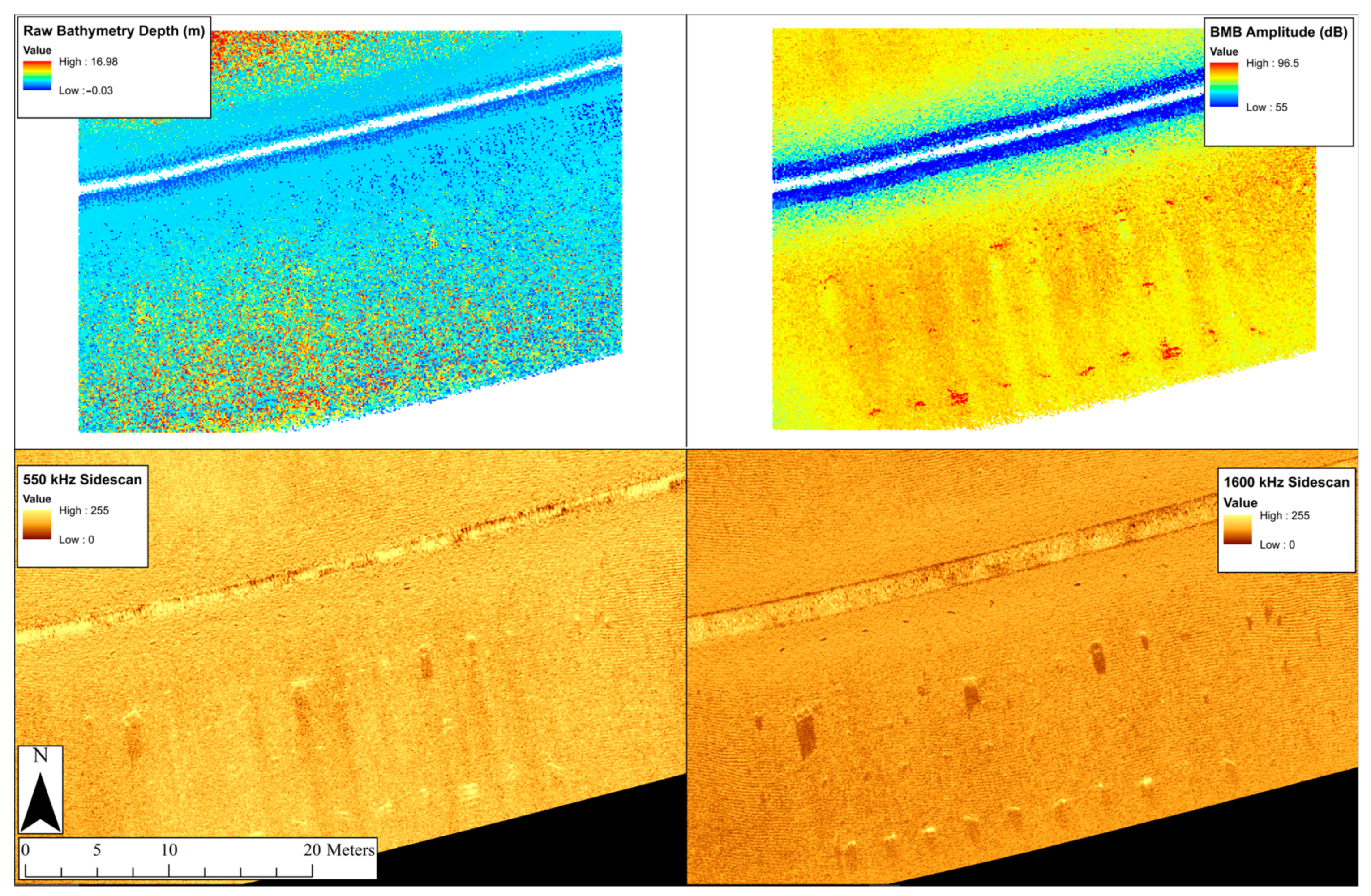
Figure 1). Borrelli et al. (2021) [5] discussed examples of the first two data sets with the instrument used here. This paper discusses the third data set as it is applied to the DCL of UXO for the ongoing project discussed above.
The BMB amplitude used in this study is not the amplitude of a singular returning waveform but a combined intensity value processed through the manufacturer’s proprietary algorithm. The amplitude used in this study is a relative data set, similar to that of sidescan backscatter. The intensity of the returning sound is not calibrated to a known reference or constant across bottom types and will be scaled dynamically throughout the range of intensities received during a specific survey. This is due to the estimation of the angle of arrival from the backscattering acoustic energy inherent with the transducer/receiver array, rather than, for example, the known angle of calibrated multibeam echo sounders (MBES) or single beam echo sounders (SBES) backscatter [22].
The instrument used in this study was an EdgeTech 6205 dual-frequency, phase-measuring sidescan sonar (PMSS). This sonar operates simultaneously collecting two frequencies of sidescan backscatter (550 kHz, 1600 kHz) and one frequency of bathymetry and BMB (550 kHz). Due to the simultaneous collection of these data, they are co-located on the seafloor and allow for increased survey efficiency negating the need for two independent systems and the challenges of combining data from two separate systems [5].
The EdgeTech 6205 is a hard-mounted setup which allows for easier shallow water surveying in water depths less than 5 m when compared to traditionally towed systems. There is a sound velocity sensor within the housing that allows for the correction for the speed of sound in water at the surface during the time of the survey with a stated resolution and accuracy of 0.001 m/s and ± 0.025 m/s, respectively (EdgeTech, 2021, West Wareham, MA, USA). Attached to the lower housing, there are independent port and starboard sonar arrays. Each of these sonar arrays are constructed with 11 piezoelectric elements, of which a single element is used for the transmission of the sound energy (EdgeTech, 2019, West Wareham, MA, USA). For sidescan data, a single transmit element and single receive element are used, allowing for the collection of traditional sidescan backscatter. For bathymetric and BMB data, a single transmit element with 10 separate receive elements for phase differentiation and angle estimation are used. All eleven elements are equally spaced at approximately one half-wavelength of the transmit frequency (EdgeTech, 2019, West Wareham, MA, USA). For this study, the single channel range was set at 20 m (40 m swath), generating a ping frequency of 69.8 Hz yielding a 14.3 ms interval.

2.2. Vessel and Ancillary Equipment

All surveys were conducted using the R/V Marindin, a modified Eastern. The vessel has an overall length of 8.2 m, with a beam of 2.5 m and typical draft of 0.6 m. This vessel is equipped with a custom mounting setup located at the bow of the vessel to allow for the deployment of the sonar, along with a Trimble R10 Real-Time-Kinematic GPS (RTK-GPS), Teledyne DMS05 motion reference unit (MRU), and HemisphereGPS VS100 vector sensors. All of the data streams are time-stamped and recorded through Discover Bathymetric, EdgeTech’s sonar data acquisition software. All electronics are powered via a 2 kW gasoline generator that provides a pure sine wave. Sound velocity profiles (SVP) are created to properly georeference the soundings with the specific speed of sound in water for the time of the survey. This is done with the internal sound velocity sensor within the EdgeTech 6205 for the surface water, as well as with a SonTek CastAway CTD, which is used to collect conductivity, temperature, and depth measurements by conducting a cast of the device through the entirety of the water column.
The objects used for DCL in this study include 60 and 81 mm mortar shells and 105 and 155 mm projectile shells, various clutter objects including, but not limited to, lobster pots, metal cylinders, cinder blocks and tires, and acoustic calibration spheres. The length and width at the widest point of all UXOs, as well as a relative size comparison can be seen in Figure 2. All UXOs in this study were provided by the DoD as inert dummies which have been deactivated with the removal of the explosive ordnance and filled with wax. The calibration spheres used are a solid aluminum alloy sphere roughly 0.09 m in diameter. These spheres can act as highly effective scatterers of sound when ensonified during surveys [3]. This is due in part to some portion of the spherical reflection surface always being perpendicular to the transducer array.

2.3. Study Site

This study focuses on the data collected during three trials from the larger study (MR19-5079)—trials 4, 5, and 6. All three trial sites for this study are on Cape Cod, MA, USA (Figure 3). Trials 4 and 5 take place in Wellfleet, MA, USA and trial 6 in Provincetown, MA, USA. Cape Cod Bay is ideal for these types of investigations due to the variability of intertidal bottom types (mud, sand, and gravel), as well as the mesotidal range (3.07 m) and semidiurnal tidal cycles that occur (NOAA, 2022). The tidal range and cycle allow for the intertidal deployment and surveying during an early morning low tide, a mid-day, high-tide vessel-based survey, and an end-of-day, low tide, re-survey and retrieval of objects within a single day.
Trial 4 at site 1 took place at Chipman’s Cove in Wellfleet Harbor, Wellfleet, MA, USA. Chipman’s Cove is a well-protected, low-energy cove within the harbor. Due to the protected nature of this area, it is able to maintain a layer sediment that behaves cohesively (Figure 4). This fine-grained material is classified here as mud, since that is the predominant bed type that the sonar will interact with. The seafloor in this location also contains many articulate shells and shell fragments, which contrast the softer, fine-grained sediments.
Trial 5 at site 2 took place at Duck Harbor beach in Wellfleet, MA, USA. Duck Harbor beach has a roughly north-to-south orientation and is fully exposed, though fetch-limited, to Cape Cod Bay to the west. This beach is a dynamic system that sees seasonal changes in its bed type, with higher energy waves removing finer-grained sediment to expose gravel beds in the intertidal region of the beachface. The prevalence of cobble-sized material was ideal for testing this method in a mixed sand and gravel setting.
Trial 6 at site 3 took place within Provincetown Harbor in Provincetown, MA, USA. The shoreline of Provincetown Harbor utilized for this study has a roughly east–west orientation. It is protected by the Provincetown Hook but is open to Cape Cod Bay to the south. This area has extensive sandy flats, which were used for this study.

2.4. Data Collection

2.4.1. Site 1, Chipman’s Cove, Wellfleet, MA, USA

Eight UXO objects were used, two of each caliber (60, 82, 105, 155 mm). The mud at the study site prevented safe access on foot; as a result, the UXOs were not precisely placed as at other sites with better access. Four UXOs, one of each size was tied together using the paracord line, with a small buoy on either end of the line for deployment and retrieval, creating two sets of four UXOs. These two lines of UXOs were deployed from the vessel onto the seafloor within the survey area.
Due to the nature of the study site, an RTK-GPS survey was not conducted. An aerial survey was conducted by a Federal Aviation Administration (FAA) licensed pilot using a DJI Phantom 4 Pro to create a high-resolution, georectified aerial mosaic and digital surface model (DSM) of the study site through structure-from-motion photogrammetry techniques. This allowed the locating of the nose and tail of each UXO from the mosaic to allow further analysis; see Borrelli et al. (this volume) for details of UAS survey methods.
Once in place, the acoustic survey team prepared track lines in a grid pattern at 5 m spacing around the study site. The close survey line spacing was designed to ensure an excessively high rate of overlap in the sidescan backscatter and a sufficient overlap for 100% coverage of bathymetric and BMB data.

2.4.2. Site 2, Duck Harbor, Wellfleet, MA, USA

Forty UXOs and nine clutter objects were used at site 2. The 40 UXOs were placed in a single north-to-south line along the gravel bed with each size class of UXO being grouped. The UXOs were aligned north to south as follows: 155 mm, 81 mm, 105 mm, 60 mm and were spaced roughly 3 m apart with varying orientations. This was done as the survey vessel could only safely travel in north-to-south directions, parallel to shore, and thus, the only way to effectively change the angle of ensonification was to change the orientation of the targets. No changes to orientations were made for the nine clutter objects. They were placed shoreward and parallel to the UXO. These clutter objects included two types of lobster pot, two metal cylinders of differing size, a cinder block, an anchor, a car tire, a boat propeller, and a set of diving weights.
Once all the objects were in place, an RTK-GPS survey was conducted using the Trimble R10. A GPS point at the nose and tail of each individual UXO, as well as points for the clutter objects were collected. This site is within the boundaries of the Cape Cod National Seashore and as such no aerial surveys were conducted at this site due to the proximity of nesting piping plovers (Charadrius melodus).
After seeding of the intertidal seafloor was completed, the acoustic surveying team planned survey lines at 5 m spacing over the study site. These survey lines ran roughly north to south along the study site. As stated above, no east-to-west lines were conducted at this site as the slope of the made it unsafe for the vessel to travel in this direction.
Once the tide was sufficiently low, the field team returned to the survey site for object retrieval. This included a repeat RTK-GPS survey of all objects to account for any movement that may have occurred throughout the tidal cycle. Once these data were collected, all objects were removed from the study site.

2.4.3. Site 3, Provincetown Harbor, Provincetown, MA, USA

Forty UXOs, fourteen calibration spheres, and eleven clutter objects were used at site 3. These objects were placed in five separate lines approximately 5 m apart in roughly a shore-parallel orientation. From north to south, 10 individual UXOs of similar caliber (60, 105, 81, and 155 mm) were placed in single lines with different orientations. In between the second and third lines of UXO were 11 clutter objects and 14 calibration spheres, the latter of which were placed in distinct patterned groups of 7 spheres each. The clutter objects used for this site include two cinder blocks, two lobster pots, a bundle of nylon line, two metal cylinders of differing sizes, a car tire, diving weights, a boat propeller, and a metal tube attached to a chain.
At site 2, once all the objects were in place, an RTK-GPS survey was conducted using the Trimble R10. In addition, an aerial survey similar to that conducted at site 1, but with many ground control points collected using the R10 helped to produce a high-resolution, geo-rectified, aerial mosaic and digital surface model (DSM) of site 3.
Once deployment data collection was complete, the acoustic survey team prepared the vessel platform and planned survey lines based on the placement of the UXO. Survey lines were prepared in a grid pattern at 5 m spacing running parallel and perpendicular to the object lines. Once the tide was sufficiently low, the field team returned to the survey site for retrieval and re-survey in the same manner as site 2.

2.5. Data Processing

The acoustic data were collected using EdgeTech’s Discover Bathymetric ver. 10.x in the JSF (.jsf) format. Data processing occurred through EdgeTech’s Discover Bathymetric ver. 10.x, Chesapeake Technology’s SonarWiz v.7 (SW7), Microsoft Excel, ESRI’s ArcMap ver. 10.8, R ver. 4.2.0, and RStudio ver. 2022.02.2. All packages in RStudio were downloaded through the Comprehensive R Archive Network (CRAN) and include mosaic, nnet, sjPlot, and readr.
Six lines of collected data from each site were used to conduct statistical analyses discussed below. The JSF data from all sites were collected in stave, or raw, format, which records the backscattering acoustic energy that return to the sonar within the given swath width for the survey, regardless of quality or filtering parameters. This allows for the reprocessing of the JSF data with variations in binning type and resolution, as well as filtering parameters within EdgeTech’s Discover Bathymetric software. Data processing methodology was first developed using site 3 data, then similar processing methods were implemented for data from sites 1 and 2 for analysis. For the purposes of this study, JSF stave data were reprocessed at the same swath range used for collection during the time of survey, 20 m for a 40 m full swath. No binning of the soundings was used to produce data representative of the native resolution of the sonar during the survey. This option allows for the representation of soundings without influence from nearby soundings in the binning process that may be more abundant or weighted more heavily in the bathymetric processing algorithms. Water column and automatic echo strength filtering was applied during the reprocessing of the data to eliminate soundings that are not representative of the seafloor or objects as this study does not aim to examine data within the water column. The signal-to-noise (SNR) filter was set to 20 dB to allow for the filtering of weak soundings. This value was selected due to the suggestion in EdgeTech’s JSF File and message description manual which states, “SNR values greater than 20 dB are excellent in terms of angle estimation quality…” (EdgeTech, 2021, West Wareham, MA, USA). The quality filter was set to 90%, which allows for the filtering of soundings that are not within the highest possible quality bin according to EdgeTech’s bathymetric processing algorithm (EdgeTech, 2021, West Wareham, MA, USA). The Outlier filter was also applied to allow for the removal of points that are deemed as outliers in EdgeTech’s bathymetric processing algorithm. This combination of processing parameters was selected so the soundings used further in the analysis were of the highest possible data quality.
Once the stave data were reprocessed in Discover Bathymetric, the individual JSF line files were imported into SW7. This software package allows for the processing of geolocated soundings and the visualization of these data through a bathymetric engine while accounting for vessel and instrument parameters and the speed of sound throughout the water column during a survey period through a process called merging. The vessel parameters for the R/V Marindin, as well as down-cast sound velocity profiles, attributed to individual survey lines based on the nearest in time, from the survey were used.
Once merged, the BMB data were processed in SW7 with no filtering or manipulation applied to the data to allow for the least altered data set possible. The data in the immediate vicinity of the objects were then exported from SW7 using the Export Bathymetry XYZ function. This function exports a csv file that contains the X, Y, Z, the amplitude of the BMB sounding in dB, the time and date of collection, and the distance from nadir for each sounding within the specified survey area, separated by the collection line number.
These individual line files were imported into ESRI ArcMap where they were consolidated into a single data set. This data set was then exported as a csv and imported into RStudio. Using the favstats function [23] for the amplitude of the six-line subset, the third quartile value of the amplitude was calculated. It was visually observed that the returning amplitude from the BMB was typically higher than the surrounding seafloor for objects. Because of this high amplitude characteristic of the soundings that fall upon objects, soundings with an amplitude lower than the third quartile value for each survey were discarded.
Navigation data from the JSF files were exported from SW7 on a per-ping basis. These navigation data include the ping date, ping time, vessel heading, and vessel attitude (pitch, roll, and heave). These navigation data were linked to the individual soundings based on the data that was nearest in time using the VLOOKUP function in Excel. This yielded a csv file for each survey line with individual soundings with attributed X, Y, Z, amplitude, date, time, distance to nadir, survey line number, vessel heading, pitch, roll, and heave values.
The csv file was reimported into ESRI ArcMap where they were classified based on their relative location to objects. For each UXO at sites 2 and 3, the deployment RTK-GPS points from the nose and tail were used to create a line shapefile representing the UXO. From this line shapefile, a 25 cm buffer was created to represent the area in which soundings would be attributed for each UXO. For calibration spheres in site 3, a 25 cm buffer was created around the deployment RTK-GPS point. Deployment RTK-GPS points for clutter objects were also connected with line shapefiles, from which a 25 cm buffer was created. For site 1, because there were no RTK-GPS points for the objects, the georectified aerial mosaic was used to select points that best represent the nose and tail of the UXO. From these selections, a 25 cm buffer was created to select points that represent the UXO. The buffer size was set at 25 cm as this value visually encompassed soundings that appeared to differ from the surrounding seafloor while also allowing for inaccuracy in the sounding’s geolocation. An analysis of sidescan backscatter data from the same data set showed a geolocation accuracy of 52 to 185 mm, with a mean of 90 mm when comparing calculated target centroids with RTK-GPS centroids [24], confirming the appropriate scale of this buffer.
Once 25 cm buffers were created for all objects, the Select by Location tool was used to select all soundings that fell within the buffers to classify them. There were three classifications used for these points: type, class, and object. This was done for all relevant objects at each site. The type classification indicated whether a point was associated with an object, regardless of what the object was or the surrounding seafloor. The class classification indicated whether a point was a UXO (inclusive of all sizes), calibration sphere, clutter object (inclusive of all clutter), or seafloor. The object classification indicated whether a point was a calibration sphere, clutter object, 155 mm UXO, 105 mm UXO, 81 mm UXO, 60 mm UXO, or the surrounding seafloor. Seafloor classifications were labeled as mud, gravel, and sand for sites 1, 2, and 3, respectively.
For all UXOs throughout the three sites, the line shapefiles from RTK-GPS points were used to calculate the heading of the UXO from nose to tail. This was done using the COGO toolkit in ArcMap. This UXO orientation was attributed to the respective soundings within the 25 cm buffer based on the individual classification. For soundings that were associated with calibration spheres, the heading was set to match that of the vessel heading taken from the navigational data. All clutter object and seafloor soundings were given an object heading of 0 as a place holder. An orientation offset between the vessel heading and orientation of objects was then calculated by subtracting the value of the object orientation from the vessel heading.
The final product of this data processing is a csv file for each survey containing BMB soundings from six lines of acoustic data, which have been filtered to just the third quartile value of the amplitude and higher. Each sounding has an associated X, Y, Z, the amplitude of the BMB sounding in dB, the time and date of collection, the distance from nadir in meters, collection line number, the per-ping vessel heading in degrees, pitch in degrees, roll in degrees, heave in meters, the type, class, and object classifications, an object orientation in degrees, and finally an object orientation offset from the vessel heading in degrees. From these data, the localization of objects can occur from the X, Y, and Z data. The detection and classification of objects will be attempted using statistical methods.

2.6. Statistical Analysis

Binomial logistic regression (BLR) and multinomial logistic regressions (MLR) were used for statistical differentiation between the seafloor types and the various objects, as well as between the objects themselves. These statistical modeling techniques are used to find the odds of an outcome variable occurring versus a baseline outcome based on selected attribute variables [25]. BLR is a type of generalized linear model which uses the logit link function to fit the maximum likelihood outcome, which will yield the odds of selecting one outcome variable over a baseline outcome variable [25].
log p X 1 p X = β 0 + β 1 X 1 + + β p X p
MLR functions similarly to BLR but allows for more than two dependent variables to be tested by using the multinomial logit link function [25].
log P r ( Y = k | X = x ) P r Y = K | X = x = β k 0 + β k 1 x 1 + + β k p x p
where X = (X1, …, Xp) are p predictors, β are model coefficients, with k categories and K being a reference category. In the case of this work, predictors would include variables BMB amplitude, distance from nadir, roll, and the orientation offset. Categories (k) would be those created with type, class, and object classifications, with the reference category (K) being specified for each test. Once selected, the predictors and all combinations of predictors for each category are analyzed by creating generalized linear models to find the best fit combinations that represent each category, and subsequently compared to the baseline category to find an odds ratio of selection to the respective category.
These statistical tests were chosen based on their ability to model probability outcomes, which in the case of this study, will give the probability of a sounding being associated with a particular object or seafloor type based on the attribute variables. The attribute variables used in the analysis were BMB amplitude (Amplitude), distance from nadir (Distance_t), roll (Roll), and the orientation offset (Offset). For all sites, the testing data were partitioned into two groups with 70% of the data being used for building the statistical models. The remaining 30% of the data was used for testing the models. These tests were run using the multinom function from the nnet package, which allows for logistic regression of two or more outcome classes. Interaction between these terms was allowed in each model so that every combination of these variables was tested. Each model was allowed to run for a maximum of 300 iterations or until convergence.
There are assumptions around data sets used with these statistical models [26], which were adhered to by the data in this study. These assumptions include independence of outcome variables, which in the case of this study means that a singular sounding cannot be both ‘Sand’ and ‘Object’ simultaneously. There is also the assumption that the attribute variables are not perfectly separated based on the outcome variables. Within this study, there is overlap in the values of all attribute variable predictors between the outcome variables, that is to say the full range of values for all attribute variables can be associated with any of the outcome variables. These statistical tests also fit these data well because there is no assumption of linearity, normality, or homoscedasticity within the data set for these tests [26].
For site 1, a single BLR model was created to differentiate between the ‘Class’ classification since only UXO were used at this site. A single MLR was created to attempt a more refined classification of soundings using the ‘Object’ designation. Due to the sample size of soundings that fall under the ‘Mud’ bed type designation being several orders of magnitude higher than ‘Object’ soundings, an additional MLR model was run excluding all soundings that were designated as ‘Mud’. This model was used to characterize ‘Object’ classifications.
For sites 2 and 3, a single BLR model was created to differentiate between the ‘Type’ classification. Two MLR models were created to attempt a more refined classification of soundings using the ‘Class’ and ‘Object’ designations described previously. For all three of these models for each site, the respective bed type was used as the reference category. Due to the sample size of soundings that fall under the respective bed type designation being several orders of magnitude higher than ‘Object’ soundings for both sites, an additional two MLR models for site 3 and additional MLR and BLR models for site 2 were run excluding all soundings that were designated as the bed type. These models were used to characterize the ‘Class’ and ‘Object’ classifications. For site 3, calibration spheres were set as the reference category when there was an elimination of ‘Sand’ soundings. For site 2, the 155 mm UXO was used as the reference category when there was an elimination of ‘Gravel’ soundings.
Classification matrices for the testing data that were run through the trained models are presented here, along with correct classification rates. The summary function in R was used to display output log odds ratios and standard errors. Using these data, Z- and P- values were calculated based on methods set forth by Blissett (2017). The log odds ratios were exponentiated to yield odds ratios that can be more easily compared. This function will present the odds ratios an X.XX…:1 output.

3. Result

The full data set from each site contained 3.0 × 10⁶, 10.9 × 10⁶, and 7.5 × 10⁶ soundings for sites 1, 2, and 3, respectively. The third quartile BMB amplitude value for each of the surveys was 83 dB, 87.5 dB, and 88 dB, for sites 1, 2, and 3, respectively. The filtered data sets contained 7.5 × 10⁵, 3.0 × 10⁶, and 2.1 × 10⁶ soundings for sites 1, 2, and 3, respectively. These data sets differ in size due to the different number of targets mapped and site accessibility with regards to possible variability of survey line orientation. The filtered amplitude ranges for each object across sites 1, 2, and 3 are represented in Figure 5, Figure 6 and Figure 7, respectively. For the box plots below, the solid black line represents the median value, with the lower and upper bounds of the gray box representing the first and third quartile value, respectively. The extension lines, or whiskers, from the box show the maximum and minimum of the data within 1.5 times the interquartile range. The small dots outside of this range represent outliers that are outside of this interquartile range.

3.1. Muddy Intertidal

Trial 4 took place on 16 October 2020, at site 1. The acoustic survey commenced at approximately 1140 h EDT and concluded at 1250 h EDT. The high tide for this day occurred at 1118 h EDT. Two casts of the SonTek CastAway CTD were conducted during the survey to measure the speed of sound through the water column during the time of survey. There were 22 sonar files that include soundings of an object collected. Once completed, the acoustic survey team retrieved the objects and returned to the dock. Three bottom grab samples were collected using a 4 L Ponar grab to perform grain size analysis and sieved using a 4 mm screen size (Table 1). The samples were processed through a Beckman Coulter LS 13 320 Particle Size Analyzer. There were no calibration spheres or clutter objects used for this site. For the table below, Table 1, as well as the other tables representing grain size information in this paper, D10, D50, and D90 represents the size of the grains in μm at the 10th percentile, 50th percentile (median), and 90th percentile of the full sample, respectively.
For site 1, when comparing all objects (in this case only UXO) to a muddy seafloor, the model created here was able to correctly classify objects 50.6% of the time (Table 2). When comparing individual UXO to the mud seafloor, the 155 mm UXO had the highest correct classification rate of 52.0% (Table 3). The 105 mm, 81 mm, and 60 mm UXOs had correct classification rates of 0.0%, 2.4%, and 15.5%, respectively, when comparing with a mud seafloor. When eliminating the seafloor soundings from the model in an attempt to differentiate between the objects themselves, the 155 mm, 105 mm, 81 mm, and 60 mm UXOs had correct classification rates of 96.8%, 60.3%, 3.8%, and 18.9%, respectively (Table 4).

3.2. Mixed Sand and Gravel Intertidal

Trial 5 took place on 13 May 2021, at site 2. The survey commenced at approximately 1250 h EDT and concluded at 1445 h EDT. The high tide for this day occurred at 1330 h EDT. Two casts of the SonTek CastAway CTD were conducted during the survey to measure the speed of sound through the water column during the time of survey. Five sediment samples were collected throughout the study site to characterize the seafloor and processed through a CAMSIZER P4 Particle Size Analyzer (Table 5). It is important to note that the sediment samples for site 2 were sieved with a 4 mm screen size to remove the larger particles as to not damage the analyzer. This results in the sediment sample classifying the underlying seafloor but not including the gravel. During the acoustic survey, 43 sonar files that include soundings of an object were collected. There were no calibration spheres used in this site.
For site 2, when comparing all objects to a gravel seafloor, the model created here was able to correctly classify objects 27.4% of the time (Table 6). When comparing all UXOs to the gravel seafloor, there was a 64.1% correct classification rate (Table 7). For individual UXO, the 155 mm UXO had the highest correct classification rate of 61.3% (Table 8). When comparing to the seafloor, clutter objects in site 2 were virtually undetectable. When eliminating gravel soundings from the models, there was a 98.1% correct classification rate for UXOs (Table 9), with the 155 mm UXO being the most distinguishable at a correct classification rate of 75.9% (Table 10). Clutter objects had a correct classification rate of 65.5% when there were no seafloor soundings present in the model.

3.3. Sandy Intertidal

Trial 6 took place on 27 May 2021, at site 3. The survey commenced at approximately 1200 h EDT and concluded at 1430 h EDT. The high tide for this day occurred at 1245 h EDT. Three casts of the SonTek CastAway CTD were conducted throughout the survey to measure the speed of sound through the water column during the time of survey. During the acoustic survey, 65 sonar files that include soundings of an object were collected. Once completed, the acoustic survey team returned to the dock. Four grain size samples were collected throughout the study site to characterize the seafloor (Table 11). During the acoustic survey, 65 sonar files that include incidence of an object were collected. For site 3, when comparing all objects to a sand seafloor, the model created here was able to correctly classify objects 52.1% of the time (Table 12). When comparing all UXOs to the sand seafloor, there was a correct classification rate of 81.2%, with clutter objects only reaching 1.9% correct classification (Table 13). When comparing individual UXO to the sand seafloor, the 81 mm UXO had the highest correct classification rate of 59.9% (Table 14). The 155 mm UXO and 105 mm UXO had rates of 49.8% and 51.0%. When eliminating seafloor soundings from the models, UXO and clutter were correctly classified 96.9% and 87.2% of the time (Table 15). When classifying objects with the removal of seafloor soundings, 155 mm UXOs were correctly classified 66.8% of the time, with calibration spheres only being correctly classified at a rate of 8.3% (Table 16).
Overall, the results from testing the models with 30% of the data will be the primary indicator of DCL for this paper. Detection will be recognized here when comparing objects to the respective seafloors. Classification will be recognized when comparing objects among themselves, both with and without the data representing the seafloor soundings present in the model.
Object detection from the soundings when compared to the surrounding seafloor occurs at an average rate of 43.4% of the time across all sites. When detecting UXO alone from the seafloor across all sites, there was an average correct classification rate of 65.3%. The 155 mm UXO had the highest classification rate, 54.4%, when comparing individual objects to the seafloor across all sites. The 105 mm, 81 mm, and 60 mm UXOs had an average correct classification rate of 17.0%, 21.4%, and 11.2%, respectively, when comparing with the seafloor across all models. Detecting clutter objects versus the seafloor for sites 2 and 3 yielded a correct classification rate of about 1%.
When looking at the models with the surrounding seafloor removed to attempt classification of the soundings, UXOs in sites 2 and 3 had an average correct classification rate of 97.5%. When differentiating between the UXOs themselves for all three sites, the 155 mm, 105 mm, 81 mm, and 60 mm UXOs had correct classification rates of 79.8%, 52.4%, 21.7%, and 16.9%, respectively. This suggests, as with other acoustic methods, that larger UXOs are generally easier to classify, possibly due to the increased number of soundings that can be associated with the objects. This shows that when eliminating the surrounding seafloor from the input data, there was an increase in average correct classification of 29%, 35.4%, 0.3%, and 5.7% for 155 mm, 105 mm, 81 mm, and 60 mm UXOs, respectively.

4. Discussion

The data presented here begin to give insights into the detection, classification, and localization (DCL) of unexploded ordnance (UXO) and other objects on the seafloor through uncalibrated BMB from phase-measuring sidescan sonar systems (PMSS). It is beyond the scope of this study to set a benchmark level at which a classification rate can be used to identify objects on the seafloor. This work was performed with the intention of producing baseline analysis on select attributes of BMB soundings for the purposes of DCL. Given the lack of studies in the peer-reviewed literature, we believe this will lay the foundation for future studies on the application of uncalibrated BMB from these instruments.
The attribute variables used in this study included amplitude, distance from nadir, roll, and the orientation offset between objects and the vessel heading. These attributes were chosen to represent the soundings based on visual observation of how the objects were being ensonified. The amplitude was the initial indicator found from this inspection due to the connection of high-amplitude soundings and objects when compared to the surrounding seafloor. Upon further inspection, this effect became more dramatic with an increase in the distance from nadir, which was then included as an attribute variable.
Overall, the detection of UXO was most effective for the 155 mm UXO, regardless of whether the seafloor was present in the model or not. This is likely because of the increased number of soundings that were associated with the object due to the proportional number of soundings within the 25 cm buffer. Due to the relative increase in size between the objects, the model would have increased sample size with which to better refine the model with larger UXOs. Although this trend could be general, it was shown that 60 mm were more correctly classified when compared to 81 mm across all sites with the seafloor soundings in the model. This could be an artifact of the chosen subset or due to the variation in soundings within the buffer for each of the respective objects. These models seem to be less effective on smaller UXOs (60 mm, 81 mm) when compared to larger UXOs (105 mm, 155 mm), both with and without the seafloor soundings present in the model, meaning these models may not currently be a suitable method of DCL for objects of these sizes.
There was also an abundance of points on objects that had a larger surface area whose long axis was oriented parallel to the sonar when compared to those that had larger surface areas that occurred perpendicular to the sonar. This led to the inclusion of the heading offset used in this study. There also appeared to be a higher abundance of soundings on larger objects that sat higher off of the seafloor. Because of this abundance of points, roll was included to account for any change in the exposed surface area of ensonification.
These results from models with the surrounding seafloor removed suggest that supervising the selection of input data by a sonar technician could improve the DCL of objects. Although Hasan et al. (2012) [27] tested several calibration methods with backscatter from an MBES for the purposes of benthic habitat mapping something similar could be done for these types of data from PMSS. This could occur by selecting areas of interest during the survey or in post processing of the data, which could potentially represent objects on the seafloor. One major benefit of using PMSS for this work is the coincidence of multiple data types which could help inform this supervised processing. This type of supervision of input data selection could also be aided by deep learning techniques, such as the use of image analysis through convolutional neural networks [28].
Along with the supervised processing of model input data, other data types, such as sidescan backscatter, could be used to help refine the models further similar to those using multispectral backscatter from MBES [29,30,31]. We believe in spite of these PMSS reflectivity data being uncalibrated, mutually beneficial research can be conducted with investigators using PMSS data and those working with MBES backscatter, such as the GeoHab working group [32].
The sidescan backscatter amplitude could potentially be correlated with the BMB amplitude to help inform object DCL, although it is important to remember that these are both relative data sets. High-quality bathymetry could be used to infer a correlation between sounding geometry and sounding attributes such as those used in this study. Although this could be done with a combination of other types of sonar arrays (MBES and SSS), the survey efficiency and colocation accuracy would likely not be as precise as with PMSS. Through this work, it was shown that the best indicator of selecting any object versus a seafloor type occurs through a combination of distance from nadir and roll (Distance_t:Roll). The odds ratios for selecting any object when compared to a seafloor type were 2.58:1, 7.16:1, and 1.87:1 for mud, gravel, and sand, respectively. This finding could also yield useful detection methods for other objects that are proud of the seafloor, such as sitting pipelines, shipwrecks, and marine debris that could critically impact surrounding habitats.
This combination of distance from nadir and roll could lead to the speculation that a grazing angle, or the angle at which the ping is interacting with the seafloor or object, could be of importance. Although exemplified in this study, the survey conditions may not be typical for future UXO detection surveys. This survey used UXOs that were proud of the seafloor due to their placement prior to acoustic surveying. However, UXOs are often partially buried, leading to grazing angles that may not reflect those of the objects in this study.
Additional attributes could also be tested with these statistical methods. There are attributes stored within the JSF files for each ping, such as a specific SNR value, that are not brought into programs such as SW7. With that, not all attributes will produce reliable results. The per-ping heave and roll values that were brought into the processed csv files were originally included in the calculation of the BLR and MLR model. The resulting odds ratios were clearly erroneous, with the ratios being orders of magnitude higher than other attributes such as the amplitude.
One issue with additional processing parameters and attributes from the EdgeTech 6205 comes from the proprietary processing and data collection methodology used by EdgeTech. As such, the user does not have full access to their algorithms. This can make the analysis of these data more complex, as well as limit the application of the BMB data and methodology presented here.
It is important to note that the results presented here are only one way of analyzing these data. Other statistical classification techniques, such as random forest or discriminant analysis, could be used with potentially differing results. There is also the possibility of applying deep learning techniques, such as multilayer or convolutional neural networks, which may be able to better recognize patterns that exist between these data [33,34]. These data also have been analyzed on a per-sounding basis, suggesting that each sounding is independent. There is the opportunity to perform clustering, or “hot-spot”, analysis on these data, which may more readily indicate the presence of an object with a cluster of high amplitude BMB soundings.
Along with other statistical measures, other data processing parameters may lead to more definitive results. The processing parameters used in this study attempt to use the highest quality data with the least amount of post-processing manipulation. There is a myriad of options when processing these data that could be explored to yield different results. Options such as empirical gain normalization in SW7 and different binning styles in Discover Bathymetric could have significant effects on the outcomes of these statistical models.
An interesting result of this study comes from the acoustic response modeling of calibration spheres at site 1. Acting as highly effective scatterers of sound, these targets would have been assumed to have had a very distinctive response, and therefore been more readily identified in the modeling process. The models presented here show poor DCL results for these objects, though they were only tested with a single seafloor type, sand. This result could be an artifact of dilution from surrounding soundings due to the size of the selection buffer used. This buffer size is potentially larger than is necessary based on the accuracy of the soundings from the PMSS system used in this study [35].

5. Conclusions

Overall, these analyses show the potential usefulness and effectiveness of phase-measured, bathymetry-mode backscatter from PMSS. It is the belief of the authors that these models yield results that are informative when attempting DCL for objects using BMB from PMSS. Due to the lack of research in current literature, results from statistical models such as these using BMB should be expanded and improved upon before any major conclusions are drawn. The results presented here give a clear indication that DCL is possible from BMB. Along with the BMB, the additional data streams from PMSS systems can help increase the application of DCL as well as address other critical needs in coastal science, such as habitat mapping, navigation, and sedimentology.
If supervised selection, or informed selection through AI techniques, of soundings or areas of interest was to be used to pick apparent objects from the full data set, UXO and clutter objects may be more easily identified than with full data set inspection. It is important to stress that the results presented here cannot definitively show DCL, as significantly more testing is needed to support and confirm the results. These results simply suggest that BMB could be used to aid in DCL efforts that are ongoing.

Author Contributions

Conceptualization, M.B.; Methodology, B.M. and M.B.; Formal analysis, B.M.; Writing—original draft, B.M.; Writing—review & editing, B.M. and M.B.; Visualization, B.M.; Supervision, M.B.; Project administration, M.B.; Funding acquisition, M.B. All authors have read and agreed to the published version of the manuscript.

Funding

This research was funded by United States Department of Defense, grant number MR19-5079.

Data Availability Statement

The data presented in this study are available on request from the corresponding author. The data are not publicly available due to ongoing analysis and publication.

Acknowledgments

We would firstly like to thank Ken Foote, without whom this work would not have been possible. His decades of expertise and experience has enabled the larger study from which this work has spun off from. We would also like to thank the Department of Defense Environmental Security Technology Certification Program (ESTCP) committee as well. Their support and funding of grant MR19-5079 has allowed this research to occur. We would like to thank everyone in the Marine Geology Department at the Center for Coastal Studies, especially Dan Solazzo and Bryan Legare. We would also like to thank Harold Orlinsky, David Finlayson, and the team from Chesapeake Technology for their help accessing and navigating SonarWiz 7 and the changes to the software that allowed this work to be possible. We would also like to thank Eric Maillard, Patrick Nissen, Richard Hill, and Mohammed Sanhaji from EdgeTech for the guidance they provided for this work. Finally, we would like to thank staff at Cape Cod National Seashore as well as the Towns of Wellfleet and Provincetown, MA, USA.

Conflicts of Interest

The authors declare no conflict of interest.

References

  1. Blondel, P. The Handbook of Sidescan Sonar; Springer Science & Business Media: New York, NY, USA, 2010. [Google Scholar]
  2. Christoffersen, J.T. Multi-Detect Algorithm for Multibeam Sonar Data; IEEE Oceans: San Diego, CA, USA, 2013; pp. 1–4. [Google Scholar]
  3. Fish, J.P.; Carr, H.A. Sound Underwater Images: A Guide to the Generation and Interpretation of Side Scan Sonar Data; Lower Cape Pub: Orleans, MA, USA, 1990. [Google Scholar]
  4. Hughes Clarke, J.E. Multibeam echosounders. In Submarine Geomorphology; Springer: Cham, Switzerland, 2018; pp. 25–41. [Google Scholar]
  5. Borrelli, M.; Smith, T.L.; Mague, S.T. Vessel-Based, Shallow Water Mapping with a Phase-Measuring Sidescan Sonar. Estuaries Coasts 2021, 45, 961–979. [Google Scholar] [CrossRef]
  6. Capperucci, R.M.; Kubicki, A.; Holler, P.; Bartholomä, A. Sidescan sonar meets airborne and satellite remote sensing: Challenges of a multi-device seafloor classification in extreme shallow water intertidal environments. Geo-Marine Lett. 2020, 40, 117–133. [Google Scholar] [CrossRef] [Green Version]
  7. LaFrance Bartley, M.; Borrelli, M. Introduction to Special Issue “Shallow Water Mapping in Coastal Environments: Recent Research, Current Technologies, and Multi-modal Approaches”. Estuaries Coasts 2022, 45, 921–922. [Google Scholar] [CrossRef]
  8. Robinson, M.; Alexander, C.; Venherm, C. Shallow Water Estuarine Mapping in High-Tide-Range Environments: A Case Study from Georgia, USA. Estuaries Coasts 2022, 45, 980–999. [Google Scholar] [CrossRef]
  9. Borrelli, M.; Oakley, B.A.; Hubeny, J.B.; Love, H.; Smith, T.L.; Legare, B.J.; Lucas, T. The Use of Multimodal Data to Augment Shallow-Water Benthic Habitat Maps for Pleasant Bay, Cape Cod, Massachusetts: Stratigraphic Data and Seafloor Maps. Northeast. Nat. 2020, 27, 48–75. [Google Scholar] [CrossRef]
  10. Brown, C.J.; Blondel, P. The application of underwater acoustics to seabed habitat mapping. Appl. Acoust. 2009, 70, 1241. [Google Scholar] [CrossRef]
  11. LaFrance Bartley, M.; Curdts, L.; Stevens, S. Procedures and Criteria for Evaluating Benthic Mapping Data: A Northeast Coastal and Barrier Network Methods Document; Natural Resource Report NPS/NCBN/NRR; National Park Service: Fort Collins, CO, USA, 2019; p. 84.
  12. Said, N.M.; Mahmud, M.R.; Hasan, R.C. Satellite-derived bathymetry: Accuracy assessment on depths derivation algorithm for shallow water area. Int. Arch. Photogramm. Remote Sens. Spat. Inf. Sci. 2017, 42, 159–164. [Google Scholar] [CrossRef] [Green Version]
  13. Simons, D.G.; Snellen, M. A Bayesian approach to seafloor classification using multi-beam echo-sounder backscatter data. Appl. Acoust. 2009, 70, 1258–1268. [Google Scholar] [CrossRef]
  14. Richardson, M.D.; Nelson, H.H.; Williams, K.L.; Calantoni, J. SERDP/ESTCP munitions response program: Underwater remediation of unexploded ordnance (UXO). In Proceedings of the Underwater Acoustics Conference and Exhibition (UACE), Hersonissos, Greece, 8–12 July 2019. [Google Scholar]
  15. Etter, D.; Delaney, B. Report of the Defense Science Board Task Force on Unexploded Ordnance; Office of the Under Secretary of Defense for Acquisition, Technology and Logistics: Washington, DC, USA, 2003. [CrossRef]
  16. Strategic Environmental Research and Development Program (SERDP). Environmental Security Technology Certification Program (ESTCP); Munitions in the Underwater Environment, State of the Science and Knowledge Gaps; SERDP: Alexandria, VA, USA, 2010. [Google Scholar]
  17. Bates, M.E.; Keisler, J.M.; Jones, E.; Linkov, I. Risky removal: Developing a holistic understanding of the risks of redeveloping sites contaminated with unexploded ordnance. Environ. Sci. Technol. 2013, 47, 3955–3956. [Google Scholar] [CrossRef] [PubMed]
  18. De Moustier, C. State of the Art in Swath Bathymetry Survey Systems. Int. Hydrogr. Rev. 1988, 65, 25–54. [Google Scholar]
  19. Grall, P.; Kochanska, I.; Marszal, J. Direction-of-Arrival Estimation Methods in Interferometric Echo Sounding. Sensors 2020, 20, 3556. [Google Scholar] [CrossRef] [PubMed]
  20. Lurton, X. Swath bathymetry using phase difference: Theoretical analysis of acoustical measurement precision. IEEE J. Ocean. Eng. 2000, 25, 351–363. [Google Scholar] [CrossRef]
  21. Mohammadloo, T.H.; Geen, M.; Sewada, J.S.; Snellen, M.; Simons, D.G. Assessing the Performance of the Phase Difference Bathymetric Sonar Depth Uncertainty Prediction Model. Remote Sens. 2022, 14, 2011. [Google Scholar] [CrossRef]
  22. Schimel, A.C.G.; Beaudoin, J.; Parnum, I.M.; Le Bas, T.; Schmidt, V.; Keith, G.; Ierodiaconou, D. Multibeam sonar backscatter data processing. Mar. Geophys. Res. 2018, 39, 121–137. [Google Scholar] [CrossRef]
  23. Horton, N.J.; Kaplan, D.T.; Pruim, R. The mosaic Package: Helping Students to ‘Think with Data’ Using, R. R J. 2017, 9, 77–102. [Google Scholar]
  24. Foote, K.G.; Borrelli, M.; Johnson, J.J.; Legare, B.; McCormack, B.; McFarland, S.; Solazzo, D. Quantifying Sidescan Sonar Positioning Accuracy, with Special Reference to Measurement in the Intertidal Zone. In Proceedings of the OCEANS 2022, Hampton Roads, VA, USA, 17–20 October 2022; pp. 1–6. [Google Scholar]
  25. James, G.; Witten, D.; Hastie, T.; Tibshirani, R. An Introduction to Statistical Learning with Applications in R, 2nd ed.; Springer Texts in Statistics: New York, NY, USA, 2021. [Google Scholar]
  26. Starkweather, J.; Moske, A.K. Multinomial Logistic Regression. 2011. Available online: https://it.unt.edu/sites/default/files/mlr_jds_aug2011.pdf (accessed on 10 April 2022).
  27. Hasan, R.C.; Ierodiaconou, D.; Monk, J. Evaluation of Four Supervised Learning Methods for Benthic Habitat Mapping Using Backscatter from Multi-Beam Sonar. Remote Sens. 2012, 4, 3427–3443. [Google Scholar] [CrossRef] [Green Version]
  28. Williams, D.P. On the Use of Tiny Convolutional Neural Networks for Human-Expert-Level Classification Performance in Sonar Imagery. IEEE J. Ocean. Eng. 2020, 46, 236–260. [Google Scholar] [CrossRef]
  29. Brown, C.J.; Beaudoin, J.; Brissette, M.; Gazzola, V. Multispectral Multibeam Echo Sounder Backscatter as a Tool for Improved Seafloor Characterization. Geosciences 2019, 9, 126. [Google Scholar] [CrossRef] [Green Version]
  30. Costa, B. Multispectral Acoustic Backscatter: How Useful Is it for Marine Habitat Mapping and Management? J. Coast. Res. 2019, 35, 1062. [Google Scholar] [CrossRef]
  31. Hughes Clarke, J.E. Multispectral Acoustic Backscatter from Multibeam, Improved Classification Potential. In Proceedings of the United States Hydrographic Conference, National Harbor, MD, USA, 16–19 March 2015; p. 19. [Google Scholar]
  32. Lurton, X.; Lamarche, G.; Brown, C.; Lucieer, V.L.; RIce, G.; Schimel, A.; Weber, T. Backscatter Measurements by Seafloor-Mapping Sonars: Guidelines and Recommendations; A Collective Report by Members of the GeoHab Backscatter Working Group. 2015, pp. 1–200. Available online: https://niwa.co.nz/static/BWSG_REPORT_MAY2015_web.pdf (accessed on 2 April 2022).
  33. Einsidler, D.; Dhanak, M.; Beaujean, P.P. A Deep Learning Approach to Target Recognition in Side-Scan Sonar Imagery. In Proceedings of the OCEANS 2018 MTS/IEEE Charleston, Charleston, SC, USA, 22–25 October 2018; pp. 1–4. [Google Scholar]
  34. Zhu, P.P.; Isaacs, J.; Fu, B.; Ferrari, S. Deep Learning Feature Extraction for Target Recognition and Classification in Underwater Sonar Images. In Proceedings of the 2017 IEEE 56th Annual Conference on Decision and Control (CDC), Melbourne, Australia, 12–15 December 2017. [Google Scholar] [CrossRef]
  35. Borrelli, M.; Legare, B.; McCormack, B.; dos Santos, P.P.G.M.; Solazzo, D. Absolute Localization of Targets Using a Phase-Measuring Sidescan Sonar in Very Shallow Waters. Remote Sens. 2023, 15, 1626. [Google Scholar] [CrossRef]
Figure 1. Comparison of sonar data types from an EdgeTech 6205 PMSS. (Top left): bathymetry. (Top right): phase-measured, bathymetry-mode backscatter (BMB). (Bottom left): sidescan backscatter (550 kHz). (Bottom right): sidescan backscatter (1600 kHz).
Remotesensing 15 01685 g001
Figure 2. Comparative sizes of UXO used throughout the study.
Remotesensing 15 01685 g002
Figure 3. Overview of study sites and their relative positions on Cape Cod (lower left), with site 1 in the (bottom right), site 2 in the (top right), and site 3 in the (top left). (Aerial photograph source: Esri, Maxar, GeoEye, Earthstar Geographics, CNES/Airbus DS, USDA, USGS, AeroGRID, IGN, and the GIS User Community).
Remotesensing 15 01685 g003
Figure 4. Example of cohesive sediments from site 1, Chipman’s Cove, Wellfleet, MA, USA.
Remotesensing 15 01685 g004
Figure 5. Site 1 BMB amplitude per individual object.
Remotesensing 15 01685 g005
Figure 6. Site 2 BMB amplitude per individual object.
Remotesensing 15 01685 g006
Figure 7. Site 3 BMB amplitude per individual object.
Remotesensing 15 01685 g007
Table 1. Site 1 grain size characteristics.
 Sample 1Sample 2Sample 3Average
D10 (μm)9.69013.179.63510.831
D50 (μm)106.0127.397.60110.288
D90 (μm)213.0342.1296.9284.018
SortingPoorly SortedPoorly SortedPoorly SortedN/A
SkewnessVery Fine SkewedVery Fine SkewedVery Fine SkewedN/A
Table 2. Site 1 class BLR with mud testing data classification results.
 Predicted MudPredicted UXO
Actual Mud221,6531309
Actual UXO 131339
% Correct classification 99.993%50.6%
Table 3. Site 1 object MLR with mud testing data classification results.
 Predicted MudPredicted 155 mmPredicted 105 mmPredicted 81 mmPredicted 60 mm
Actual Mud221,656565306293150
Actual 155 mm464282236197
Actual 105 mm30020
Actual 81 mm32201425
Actual 60 mm0514168
% Correct Classification99.995%52.0%0.0%2.4%15.5%
Table 4. Site 1 object MLR without mud testing data classification results.
 Predicted 155 mmPredicted 105 mmPredicted 81 mmPredicted 60 mm
Actual 155 mm1195136354293
Actual 105 mm023413338
Actual 81 mm36122226
Actual 60 mm367783
% Correct Classification96.8%60.3%3.8%18.9%
Table 5. Site 2 grain size characteristics.
 Sample 1Sample 2Sample 3Sample 4Sample 5Sample 6Average
D10 (μm)287.1240.1250.6258.4344.7274.1275.8
D50 (μm)597.7452.7554.1560.5607.6640.8568.9
D90 (μm)1413.6698.01353.31389.91745.31714.81385.8
SortingModerately SortedModerately Well SortedModerately SortedModerately SortedModerately SortedPoorly SortedN/A
SkewnessSymmetricalFine SkewedSymmetricalCoarse SkewedCoarse SkewedCoarse SkewedN/A
Table 6. Site 2 type BLR testing data classification results.
 Predicted GravelPredicted Object
Actual Gravel867,78516,137
Actual Object1066075
% Correct classification 99.988%27.4%
Table 7. Site 2 class MLR with gravel testing data classification results.
 Predicted GravelPredicted UXOPredicted Clutter
Actual Gravel867,79858295963
Actual UXO 9310,4190
Actual Clutter010
% Correct classification 99.989%64.1%0.0%
Table 8. Site 2 object MLR with gravel testing data classification results.
 Predicted GravelPredicted 155 mmPredicted 105 mmPredicted 81 mmPredicted 60 mmPredicted Clutter
Actual Gravel867,81922562397141513045963
Actual 155 mm436481264187815670
Actual 105 mm6200030
Actual 81 mm023176460
Actual 60 mm61901402470
Actual Clutter010000
% Correct Classification99.992%61.3%0.0%1.8%7.9%0.0%
Table 9. Site 2 class BLR without gravel testing data classification results.
 Predicted UXOPredicted Clutter
Actual UXO 15,9342057
Actual Clutter3153906
% Correct classification 98.1%65.5%
Table 10. Site 2 object MLR without gravel testing data classification results.
 Predicted 155 mmPredicted 105 mmPredicted 81 mmPredicted 60 mmPredicted Clutter
Actual 155 mm4516148322891706612
Actual 105 mm3711637550682151
Actual 81 mm19226258
Actual 60 mm1037115331616
Actual Clutter9384654434185176
% Correct Classification75.9%44.5%1.8%10.1%86.8%
Table 11. Site 3 grain size characteristics.
 Sample 1Sample 2Sample 3Sample 4Sample 5Sample 6Average
D10 (μm)521.8530.9512.0558.8559.8531.6535.816
D50 (μm)804.3807.1772.4868.9867.8811.4821.999
D90 (μm)1481.71431.71346.91565.31563.81539.11488.066
SortingModerately Well SortedModerately Well SortedModerately Well SortedModerately Well SortedModerately Well SortedModerately Well SortedN/A
SkewnessCoarse SkewedCoarse SkewedCoarse SkewedCoarse SkewedCoarse SkewedCoarse SkewedN/A
Table 12. Site 3 type BLR testing data classification results.
 Predicted SandPredicted Object
Actual Sand615,40510,860
Actual Object58811,810
% Correct classification 99.905%52.1%
Table 13. Site 3 class MLR with sand testing data classification results.
 Predicted SandPredicted UXOPredicted Calibration SpherePredicted Clutter
Actual Sand615,721268906294
Actual UXO 10911,645187142
Actual Calibration Sphere0000
Actual Clutter16340125
% Correct classification 99.956%81.2%0.0%1.9%
Table 14. Site 3 object MLR with sand testing data classification results.
 Predicted SandPredicted 155 mmPredicted 105 mmPredicted 81 mmPredicted 60 mmPredicted Cal. SpherePredicted Clutter
Actual Sand615,7651261661674664116305
Actual 155 mm52255356150088781031
Actual 105 mm86041705134194140
Actual 81 mm053041919547643960
Actual 60 mm06700265780
Actual Cal. Sphere01120001620
Actual Clutter16800040125
% Correct Classification99.963%49.8%51.0%59.9%10.2%8.7%1.9%
Table 15. Site 3 class MLR without sand testing data classification results.
 Predicted Calibration SpherePredicted UXOPredicted Clutter
Actual Calibration Sphere000
Actual UXO187113,896824
Actual Clutter04425637
% Correct Classification0%96.9%87.2%
Table 16. Site 3 Object MLR without sand testing data classification results.
 Predicted Calibration SpherePredicted 155 mmPredicted 105 mmPredicted 81 mmPredicted 60 mmPredicted Clutter
Actual Calibration Sphere156960000
Actual 155 mm81034239359131092623
Actual 105 mm4086881751136170
Actual 81 mm38349239919457630
Actual 60 mm11425757825620
Actual Clutter01712041861695838
% Correct Classification8.3%66.8%52.3%59.6%21.6%90.4%
Disclaimer/Publisher’s Note: The statements, opinions and data contained in all publications are solely those of the individual author(s) and contributor(s) and not of MDPI and/or the editor(s). MDPI and/or the editor(s) disclaim responsibility for any injury to people or property resulting from any ideas, methods, instructions or products referred to in the content.

