Abstract
Spatial downscaling is an important approach to obtain high-resolution land surface temperature (LST) for thermal environment research. However, existing downscaling methods are unable to sufficiently address both spatial heterogeneity and complex nonlinearity, especially in high-resolution scenes (<120 m), and accordingly limit the representation of regional details and accuracy of temperature inversion. In this study, by integrating normalized difference vegetation index (NDVI), normalized difference building index (NDBI), digital elevation model (DEM), and slope data, a high-resolution surface temperature downscaling method based on geographically neural network weighted regression (GNNWR) was developed to effectively handle the problem of surface temperature downscaling. The results show that the proposed GNNWR model achieved superior downscaling accuracy (maximum R2 of 0.974 and minimum RMSE of 0.896 °C) compared to widely used methods in four test areas with large differences in topography, landforms, and seasons. We also achieved the best extracted and most detailed spatial textures. Our findings suggest that GNNWR is a practical method for surface temperature downscaling considering its high accuracy and model performance.
1. Introduction
High-resolution land surface temperature (LST) products play a crucial role in various types of environmental research. The existing applications mainly include urban heat island effect research [1], climate change monitoring [2], soil moisture estimation [3], surface flux estimation [4], forest fire monitoring [5], drought monitoring [6], surface carbon inversion [7], and geological resource exploration [8]. The acquisition of high-quality high-resolution LST data is particularly important for the development of those research areas.
With the development of remote sensing technology, spaceborne thermal infrared sensors are able to obtain data globally [9]. They provide a convenient and effective way to acquire thermal infrared data by remote sensing satellite. However, due to the limitation of thermal infrared sensor performance, it is difficult to obtain high-resolution thermal infrared data for research. As one of the core topics of remote sensing, spatial downscaling can help researchers obtain more high-resolution data, which is widely used in various remote sensing research fields, such as precipitation [10,11], water storage [12,13,14,15,16,17], and LST [18,19]. At present, the downscaling thermal infrared remote sensing image has become the main data source for high-resolution LST and thermal environment research. The methods of obtaining high-resolution LST based on satellite thermal infrared remote sensing data can be roughly divided into two categories: statistical model-based downscaling methods, and image fusion-based downscaling methods [20]. Common image fusion-based methods include the generalized Laplacian pyramid (GLP) method [21], the co-kriging interpolation method [22], and Bayesian methods [23]. Compared to image fusion-based downscaling methods, statistical model-based downscaling methods for LST are easier to operate, and their downscaling results are accurate within an acceptable range, making them the most widely used. Statistics-based methods are based on the assumption of “relationship scale invariance”. The key to successful downscaling is to deal with the spatial non-stationarity and complex nonlinearity in the complex regression relationship of “the LST-surface factors”, and common algorithm models include the DisTrad (disaggregation procedure for radiometric surface temperature) downscaling algorithm [24], the TsHARP (Thermal sHARPening) algorithm [25], the Geographically Weighted Regression (GWR) algorithm [26], and the Multi-scale Geographically Weighted Regression (MGWR) downscaling algorithm [27]. In addition, applications of machine learning algorithms into this area are being developed [28], such as the random forest (RF) algorithm [29]. Although those statistics-based methods are widely used, they each have disadvantages. Traditional statistical models struggle to handle non-linear problems, while machine learning models face challenges in handling local spatial non-stationarity [30], which limits their ability to construct expressions for complex natural phenomena with significant spatiotemporal variability of LST, so that the model accuracy and visual effects are not satisfactory. In high-resolution scenes, due to the increase in the number of pixels and the demand for spatial details, the regression relationship between “the LST-surface factors” will become more complex, and the accuracy of the regression results should also be higher. In addition, “the thermal mixture effect” in hot pixels also makes downscaling more difficult [31]. To obtain high accuracy and reasonable high-resolution surface temperature, it is increasingly urgent to develop new and operational models that can handle spatial non-stationarity and complex nonlinearity in LST regression statistics.
Du et al. [32] recently proposed a Geographically Neural Network Weighted Regression (GNNWR) model, which combines the advantages of the Ordinary Liner Regression (OLR) and Neural Network models. By using the learning ability of neural networks and the local spatial interpretation ability of spatial weight, this model can deal with the spatial heterogeneity and complex nonlinearity of regression relationships, which has better fitting accuracy and prediction performance than the GWR and neural network models, with the potential to solve complex spatial relationships in many fields [33,34,35]. Specifically, the GNNWR model uses a spatially weighted neural network (SWNN) to replace the kernel function of GWR, so that the GNNWR model shows excellent interpretation ability in spatial non-stationary modeling, and its application in the study of LST downscaling can provide a new solution for improving the precision of LST downscaling and strengthening the spatial details of downscaling data.
Therefore, our goal is to construct a high-resolution LST downscaling model based on GNNWR and demonstrate its superiority. In the model, Normalized Differential Vegetation Index (NDVI), Normalized Difference build-up Index (NDBI), DEM, and Slope serve as covariates to achieve accurate fitting of spatial heterogeneity and nonlinear features in the regression relationship between LST and multiple factors so as to obtain high-precision downscaling results of regional LST. Moreover, the downscaling accuracy of TsHARP, RF, GWR, and MGWR algorithms was quantitatively compared, and the universality of the constructed model was evaluated in different spatiotemporal environments. Moreover, Landsat8 Ready Analysis Data (ARD) were added to compare and evaluate the visual effects of downscaling model results. In other words, this study aims to prove from various aspects that the proposed GNNWR model has the best availability and accuracy, with the best reasonability and practicability in LST downscaling.
2. Materials
2.1. Study Area
In this study, Kansas City (study area A) and Phoenix (study area B) were selected as the study areas, the locations of which are shown in Figure 1. Study area A is located in the western part of Missouri, at the confluence of the Missouri River and the Kansas River. It is a typical plain landform with high vegetation coverage, as the mainland is covered by grassland and sparse forest. The climate in this area is temperate continental humid with four distinct seasons, which can represent most temperate areas in the Midwest of the United States. Study area B is located in the middle of Arizona, with a predominant land cover of bare soil. This area features a subtropical desert climate with low rainfall.
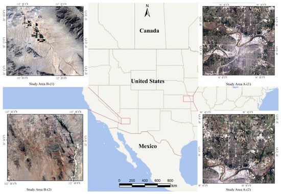
Figure 1.
Location of the study area. The study area A is located in Kansas City, while the study area B is located in Phoenix.
In addition, February was selected as the winter sample and July the summer sample. Details are shown in Table 1 and Table 2. The study areas cover common landform and land cover types, as well as winter and summer seasons, with a large span of surface temperatures, which is conducive to the study of the complex spatiotemporal relationship of downscaling LST.

Table 1.
Basic information of study areas. This table displays the study areas’ code, image acquisition time, and geomorphological features.
Table 2.
Regional average, maximum and minimum LST.
2.2. Data
NDVI has been widely used in the downscaling process of LST [36]. DEM and Slope are the key factors reflecting the differentiation of spatial thermal patterns under altitude differences [37], which indicates that the relationship model with LST can be well constructed by integrating factors such as NDVI, DEM, and Slope. Based on the above three factors, this paper adds NDBI as the independent variable input of the model. NDBI is easily affected by such factors as sparse vegetation and bare soil and can fill the deficiency of the representation of impervious surfaces in NDVI. The main factor data sources in this study were Landsat8 red band (R), near-infrared band (NIR), short-wave infrared band (SWIR1), thermal infrared band 10 (TIRS1), and NASA DEM. The experimental data are shown in Table 3, which mainly includes the data name, variable name, spatial resolution, and data source.
Table 3.
The details and source of all factors.
- (1)
- NDVI is sensitive to vegetation cover, with a value range of [−1, 1], indicating the presence of vegetation cover and increasing with the coverage degree. In this study, it was calculated from the Landsat 8 red band (R) and near-infrared band (NIR). The calculation formula is as follows:
- (2)
- NDBI is sensitive to impervious surfaces and has a value range of [−1, 1]. It can accurately reflect information on built-up land, with higher values indicating higher proportions and densities of built-up land. In this study, NDBI was calculated using Landsat 8 Near Infrared (NIR) and Shortwave Infrared 1 (SWIR1) bands.
- (3)
- DEM. Obtained by clipping NASA DEM data.
- (4)
- Slope. Obtained by using ArcGIS default slope analysis, with DEM data as the input raster.
- (5)
- Land surface temperature. Obtained from Landsat 8 thermal infrared band 10-TIRS using the mono-window algorithm proposed by Qin [38].where T represents LST (°C), Ts represents the brightness temperature (/K) of the sensor, Ta represents the average atmospheric temperature (/K), and a and b are reference coefficients. When the LST is between 0 and 70 °C, the values of a and b are −67.355351 and 0.458606, respectively. C and D are intermediate variables, which are calculated using the following formula:where is the emissivity of the surface, which is obtained according to Qin’s empirical formula, and is the total atmospheric transmittance from the ground to the sensor, provided by NASA.
Based on the above data, this study aimed to obtain spatial downscaling results of LST with a spatial resolution of 30 m. However, due to the different sources of the above data, problems such as inconsistent projection information and different spatial resolution still existed. To establish the relationship between the spatial resolution of LST and surface factors, all factors were uniformly converted into the same projection coordinate system (WGS_1984_UTM). A 100 m grid was used as the spatial resolution to carry out data matching and the nearest resampling, and the spatial connection method was used to integrate all data into the same grid unit. A group of argument variables with a specification grid as the unit was formed.
3. Methods
3.1. Land Surface Temperature Downscaling Model Based on GNNWR
According to the “invariant relationship scale” hypothesis, downscaling of LST generally involves establishing a functional relationship between LST and surface factors at low resolution and then applying this regression function to high-resolution scenarios, along with residual correction, to obtain the predicted results. In this study, the relationship is shown by the following equation:
where represents the functional relationship between LST and surface factors at low resolution, and is the regression residual. Then, the surface factors at high resolution are input into the regression function, and is the desired result.
GNNWR obtains a spatial downscaling model of LST by constructing a functional relationship between LST and physical parameters at low spatial resolutions and then applying it to high spatial resolutions. However, unlike previous methods, GNNWR does not need to interpolate the residuals for model calibration [39].
Based on the geographical weighting idea similar to GWR, the GNNWR model considers the spatial variability of the regression relationship as the fluctuation level of the “OLR regression relationship” due to spatial non-stationarity at different locations. In this study, four factors, namely, NDVI, NDBI, DEM, and slope, were used. Therefore, in the LST downscaling experiment of this study, the GNNWR model structure is defined as follows:
where = represents the spatial coordinates of the i-th sample point; the regression coefficients of the OLR model, denoted by β = (β0, β1, …, β4), signify the overall level of the regression relationship between LST and the covariates across the entire study region.
The estimated matrix of the OLR coefficients is expressed as follows:
where
where n represents the number of samples. So, substituting the OLR estimate into Equation (8), we have :
where W(si) is a (1 + k) × (1 + k) diagonal matrix representing the geographical weights. k is the number of independent variables and can be expressed as:
To capture the intricate interplay between spatial distance and spatial weight with precision, GNNWR devises a spatially weighted neural network that expresses the weight kernel function. More specifically, the SWNN leverages the estimated spatial distance between the prediction point and all modeling sample points as its input layer and generates the spatial weight matrix as the output layer, while flexibly adapting to the modeling requirements by selecting an appropriate number of hidden layers. Ultimately, the spatial weight of the prediction point i can be computed through the following formula:
where is the Euclidean spatial distance from the point to the set of samples. Therefore, the LST downscaling model based on GNNWR is defined as shown in Figure 2.
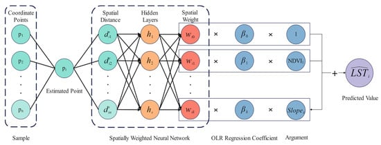
Figure 2.
Definition of the GNNWR land surface temperature downscaling model.
3.2. Model Design and Implementation
To improve the optimization efficiency and solution capability of the spatially weighted neural network in the GNNWR model, a neural network architecture and implementation strategy was designed, as shown in Figure 3.
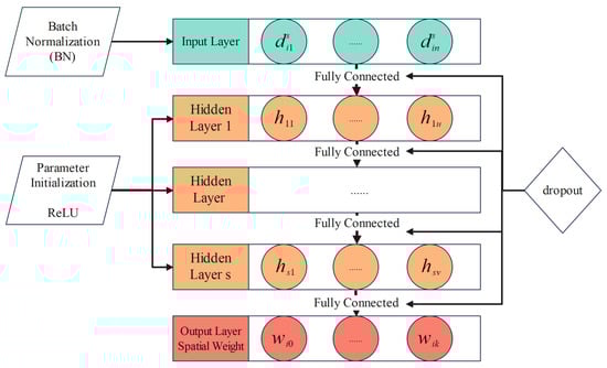
Figure 3.
GNNWR neural network architecture and implementation strategy.
The spatial weighted neural network uses fully connected networks between each layer and applies the dropout technique proposed by Srivastava [40] to improve the model’s generalization ability. In addition, each hidden layer uses the parameter initialization method proposed by He et al. [41] and the rectified linear unit (ReLU) activation function to improve the model’s optimization efficiency. At the same time, to reduce the influence of internal covariate shifts, batch normalization technology is introduced into the hidden layer to further improve the calculation ability of the GNNWR model [42]. Regarding the number of neurons in each layer, this study utilized a neural network architecture comprised of seven layers, including one input layer, five hidden layers, and one output layer. The specific parameters used in this architecture are detailed in Table 4.
Table 4.
Details of neural network parameter settings.
Figure 4 illustrates the training and validation process of the GNNWR model in which the dataset is partitioned into three subsets in an 8:1:1 ratio, namely, the training set, validation set, and test set, through random selection. The random division of data should make the three data subsets cover the whole research area, thereby minimizing the estimation bias arising from sample selection differences and enhancing the robustness and reliability of the model. Notably, the OLR regression coefficient denoting the average relationship is computed from the training set, which is primarily used to optimize the network weights and biases of the SWNN during the model training process. Moreover, the validation set is employed to monitor the overfitting of the model after each training epoch, whereas the test set is employed to evaluate the predictive performance of the model, both of which are excluded from the model training process [43].
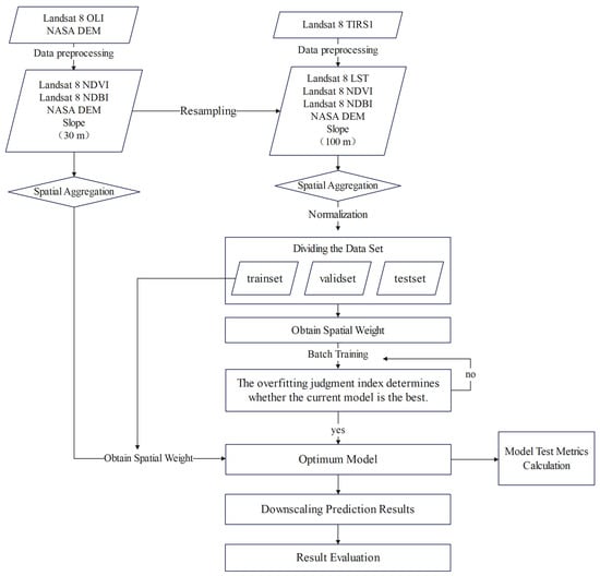
Figure 4.
Implementation process of the GNNWR model.
In this study, MSE was adopted as the loss function of the GNNWR model, and the MSE of the verification set was used as the overfitting evaluation index [33]. If the overfitting metric exhibits a persistent increasing or plateauing trend and exceeds the predetermined EarlyStop threshold, the model is deemed overfitting and the training process is terminated.
3.3. Model Evaluation
This study compared several representative downscaling algorithms for LST, including RF, TsHARP, GWR, and MGWR. Except for TsHARP using single-factor NDVI as the regression kernel, all other algorithms use the same factors as GNNWR.
This study applied five commonly used indicators, including the coefficient of determination (R2), root mean square error (RMSE), peak signal-to-noise ratio (PSNR), mean absolute error (MAE), and mean absolute percentage error (MAPE), in evaluating and comparing the spatial downscaling model accuracy of LST.
where represents the observed value, represents the predicted value, and represents the mean value of the observed values.
4. Results
4.1. Comparison and Analysis of Model Performance
This study used five performance evaluation metrics, namely, R2, RMSE, MAPE, PSNR, and MAE, to quantitatively evaluate the regression accuracy and fitting effect of the model and to compare the performance of the five models. Table 5 illustrates the specific regression evaluation indicators of the five downscaling algorithm models.
Table 5.
Regression evaluation metrics for different downscaling models.
Among the four study areas, the GNNWR model showed higher accuracy, followed by the GWR and MGWR models, but with slight variations. In Area A, GWR performed better than MGWR, while in Area B, MGWR was superior to GWR. The GNNWR model demonstrated improved regression accuracy compared to both the MGWR and GWR models. For instance, compared to the best-performing models in each study area, the R2 of the GNNWR model respectively increased by 0.025, 0.029, 0.009, and 0.012, and the RMSE respectively decreased by 2.33%, 4.91%, 4.49%, and 9.31%. The R2 was above 0.9 in all three study areas, and the RMSE was mostly around 1 °C, with values less than 1 °C in three areas. Among them, the best-performing Area B-(2) had the highest R2 and the smallest RMSE, which were, respectively, 0.974 and 0.896. Additionally, the GNNWR model showed average reductions of 5.73% and 5.34% in MAPE and MAE, respectively, and an increase of 2.445% in PSNR. These three models were superior to the RF and TsHARP models in terms of evaluation metrics. Figure 5 demonstrates the regression evaluation indexes of the GNNWR model, the MGWR model, and the GWR model in detail.
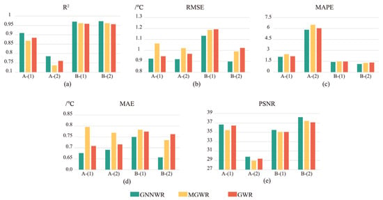
Figure 5.
Comparison of performance metrics of different downscaling models. (a–e) show R2, RMSE, MAPE, MAE, PSNR indicators of the GNNWR model, the MGWR model, and the GWR model respectively.
As seen in Figure 5, the GNNWR model had good performance in three areas, namely, A-(1), B-(1), and B-(2), with good R2 and error metric evaluations. However, all models’ R2 values in the A-(2) region were slightly lower, which may be related to the heterogeneity of the region itself. Similarly, the models in the A region performed worse than those in the B region, indicating that the interpretation of spatial non-stationarity in complex terrains requires the consideration of more factors than in simpler terrains. This also indirectly indicates that the models’ ability requirements are higher in complex terrains. Overall, the GNNWR model had the best performance in all indicators, and its performance was less affected by perturbations in different study areas, indicating good stability and an excellent capturing ability for spatial non-stationarity and complex nonlinearity.
In terms of computation time, the order of models from fastest to slowest was TsHARP < RF < GWR < GNNWR << MGWR. However, except for GNNWR, all other models still required residual transformation interpolation to complete the downscaling process. Therefore, the total downscaling time for GNNWR was much shorter than that for the other models.
The 30 m GNNWR model regression results were resampled to 100 m and compared with the inverted LST data to analyze the absolute errors in each region. The error pixels were classified into 5 levels, namely, 0–1 °C, 1–2 °C, 2–3 °C, 3–4 °C, and >4 °C, and the proportion of pixels in each error level was calculated. The results are shown in Figure 6.
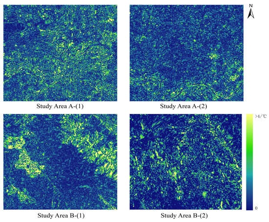
Figure 6.
The result of GNNWR absolute error visualization.
From Table 6, it can be seen that around 60% of the pixels in the four study areas had errors within the 0–1 °C range, indicating that GNNWR had good accuracy in downscaling the surface temperature in different topographic regions and seasons. Errors >2 °C accounted for 12.66%, 5.29%, 3.44%, and 14.54% of the total pixels in the four study areas and were mainly distributed in areas with intensive human activities, such as urban and riverside regions, as well as mountainous regions where the model algorithm’s outliers were mainly located on the mountain ridges and valleys due to differences in elevation. In addition, the overall proportion of absolute error pixels in study area A-(2) was relatively good. However, combined with Figure 5, it can be seen that this area had a relatively large MAPE, indicating a significant level of error. The main reason is that the explanatory power of the independent variables in study area A-(2) was insufficient, such as the NDVI values not showing significant differences in winter, and trees being not as lush as in summer. Therefore, it may be necessary to replace or add more reasonable regression covariates to the model.
Table 6.
Proportion of GNNWR results’ absolute error pixels.
4.2. Spatial Distribution of High-Resolution Land Surface Temperature
To better analyze the downscaling results, this study compared the visual effects of Landsat8 ARD surface temperature product data, GNNWR downscaling results, and other models that performed well in each region in the four selected study areas. The Landsat 8 ARD surface temperature product is a high-resolution dataset (30 m) generated by the USGS through the reanalysis of Landsat 8 thermal infrared data applying georeferencing, atmospheric correction, and resampling techniques. Figure 7 shows the overall comparison of surface temperature in the four main study areas.
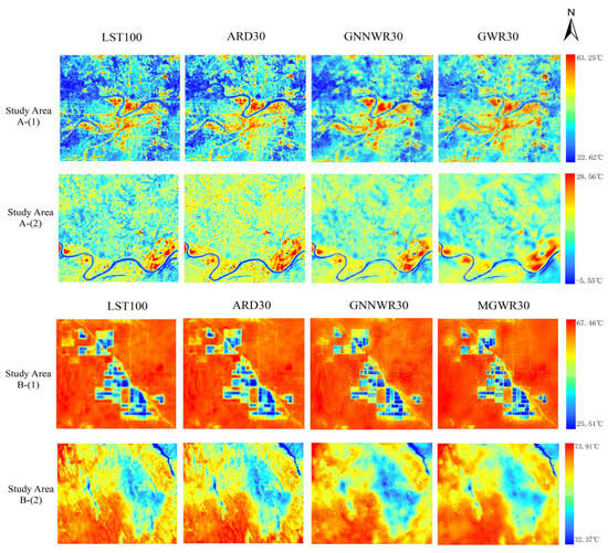
Figure 7.
Overall comparison of downscaling results for main study areas.
It can be seen from Figure 7 that the GNNWR downscaling results were in line with the original information of most LST, with more detailed and richer spatial textures. This indicates that while the model method achieved good results, it also maintained the consistency of the thermal characteristics distribution before and after downscaling. Especially in the B-(1) research area with flat and single topography in summer and the B-(2) research area with high altitude difference and single topography in summer, the regression results of the GNNWR downscaling model had good and reasonable visual detail effects. Compared with the ARD LST product, the GNNWR downscaling results had better spatial details, and the ARD LST product was an obvious resampled product. Compared with the better models in each study area, the LST distribution of the GNNWR downscaling results was more reasonable. For example, in the B-(1) and B-(2) regions, GNNWR did not have errors as did the MGWR model, which presented a large-scale data overestimation. In addition, GNNWR’s results showed that in study area A, high-temperature areas are mainly concentrated in urban areas and higher than surrounding areas, indicating obvious urban heat island effects, while in study area B, due to the characteristics of desert areas, low temperatures are mainly concentrated around urban or high-altitude areas, which, in these areas mentioned above, shows that the LST obtained from GNNWR was basically consistent with satellite-retrieved LST.
5. Discussion
5.1. Availability and Advantages of the GNNWR Model
Considerable progress has been made in satellite data downscaling. However, the current methods based on statistical models cannot simultaneously deal with the spatial non-stationarity and complex nonlinearity of the LST-surface factors relationship, which makes it difficult to obtain reasonable and accurate downscaling results, especially in the region of complex topography. Therefore, a GNNWR-based LST downscaling method was developed in this study to obtain high-precision and reasonable LST data.
It can be seen from Table 5 that the GNNWR model has the best performance, followed by the GWR and MGWR model, which have their advantages in each region and are far superior to the TsHARP and RF models. In particular, the bandwidth of each factor in the results of the MGWR model in study area A is equal, indicating that MGWR degenerates into GWR in complex landforms, which is not fully applicable to downscaling applications in this case because of its instability. At the same time, GNNWR has higher index accuracy than GWR and MGWR. For example, RMSE, MAPE, and MAE of the GNNWR model decreased by 5.26%, 5.73%, 5.34%, respectively, and PSNR increased by 2.445% on average, and the maximum R2 reached 0.974. All these indicate that GNNWR has superior performance in constructing the LST and surface factors relationship. This also shows that the SWNN weight matrix of GNNWR is superior to the kernel function of GWR in space non-stationarity expression. In addition, in the comparison of image vision, the GNNWR model has a more accurate description and better expression of spatial details in the expression of ground object features and is more reasonable locally, which further proves the applicability of GNNWR in LST downscaling.
Using the GNNWR model for downscaling, reasonable design of deep learning model parameters can achieve excellent results, and it is more operational and theoretical, not only expressing the ability to cope with complex spatial non-stationarity but also compatible with the powerful computing power of deep learning. Therefore, it can be used for further research and testing of multi-region, multi-factor, and multi-data sets for common surface temperature downscaling scenarios based on “relationship scale invariance” to improve the universality and accuracy of model methods.
5.2. Veracity and Reasonability of LST Mappings
To better display the experimental results and assess the accuracy and reasonability of LST mappings of GNNWR, Figure 8 shows the comparison details in each area.
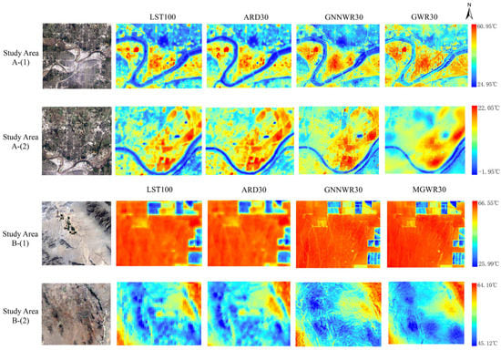
Figure 8.
Detailed comparison of downscaling results.
Upon examining the details in each study area, the thermal spatial distribution of each model or product is basically consistent. However, it is evident that the GNNWR model exhibits more reasonable and detailed temperature distributions for most land surfaces compared to other high-performing downscaling models. The GNNWR model outperforms other high-performing downscaling models in terms of not producing unrealistic temperature distributions, smooth color patterns, overall numerical abnormalities, or failing to express the geographic features of roads, buildings, and dense forest areas in complex terrain, such as rivers in region A-(1) and ridges in region B-(2). Although the high-performing GWR and MGWR models have achieved downscaling effects, they sometimes exhibit indistinctive and overly smooth land features, lack of details, and large-scale temperature estimation deviations. Specifically, in A-(1) and B-(1) regions, the regression results of the GWR model and the MGWR model show obvious “overestimation” in the river part and the plain part, respectively, while the regression results of the MGWR model show obvious “underestimation” in the hillside part in B-(2). Moreover, in the A-(2) region, a large colorful glossy area appears. At the same time, these unreasonable distributions also illustrate GNNWR’s excellent regression prediction ability and high estimation accuracy. Figure 9 visualizes the absolute errors of the regression results of the GNNWR model and the model with better performance in each study area at a spatial scale of 100 m.
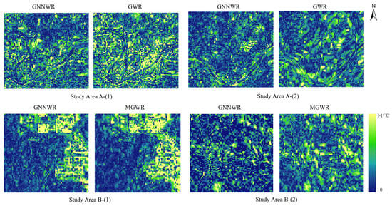
Figure 9.
At a resolution of 100 m, absolute error visualizations of the GNNWR and well-performing model in each detail area of Figure 8 compared with the retrieved LST.
From Figure 9, it can be observed that the errors of each model are mainly concentrated in densely populated areas such as cities and riverbanks, as well as in mountainous areas such as ridges, and the error proportions are relatively high in the GWR and MGWR models, which are consistent with our previous findings. In addition, the PSNR index of GNNWR in Table 5 is mainly between 30 and 40 and has the highest level, indicating that the GNNWR model also performs better in terms of quantitative visual accuracy. In summary, compared to other models, GNNWR results are more reasonable and accurate.
5.3. Model Applicability of Different Factors and Sensors
It can be seen from Table 5 that in the winter complex landform, the effect of NDVI weakens, and the regression fitting accuracy of the model decreases, which indicates that the effectiveness and selection of regression factors may lead to changes in the model’s ability to explain the real LST. After eliminating the interference of the autocorrelation among the factors, the model’s expressive power can be enhanced by adding suitable surface factors for complex terrain. In areas with dense vegetation, NDVI has a greater impact on the results during the downscaling process. In urban areas, NDBI plays a greater role in reflecting the surface dryness index. After canceling the NDBI factor, this study also conducted GNNWR downscaling analysis on the study area A-(1), as shown in Figure 10. Comparing the downscaling temperature prediction results in Table 5, it can be seen that, in addition to the commonly used factors of elevation and slope, the model’s accuracy using the combined NDBI + NDVI is higher than that using only NDVI. Similarly, for different complex terrains and seasons, using surface factors that can represent distinct features of the area, such as slope direction, the normalized difference water index (NDWI), and the normalized difference bare soil index (NDBSI), endows the model with better interpretability for specific regions.
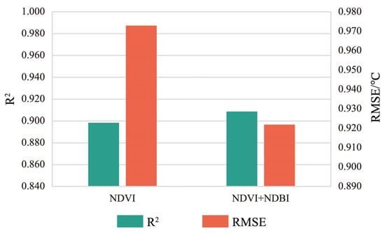
Figure 10.
Comparison of R2 and RMSE of GNNWR downscaling results using different combinations of covariates.
As for data sources, currently, data from different satellite sensors are commonly used to obtain high temporal and spatial resolution surface temperatures. The imaging time and imaging methods of different sensors differ, resulting in differences in the produced surface temperature. Therefore, when establishing a regression relationship at a lower resolution, it will inevitably be affected by different variables. For example, when downscaling using MODIS data, the LST values are derived from the Terra/MODIS sensor, while the NDVI values are obtained from the OLI sensor of Landsat 8. As the two sensors have significant differences in various aspects, such discrepancies will result in errors in the final downscaling products. However, from the perspective of the regression model alone, the accuracy of the GNNWR model is still higher than traditional downscaling methods and machine learning methods. The next step is to apply the model to downscaling between different sensors.
6. Conclusions
By integrating four land surface factors as the independent variables in different seasons, elevations, and land cover types in the research area, this study proposes a high-resolution (<120 m) LST downscaling method based on GNNWR, which can well represent spatial heterogeneity and complex nonlinearity. The modeling accuracy is compared with four commonly used downscaling methods, and the visual effect is compared with the Landsat 8 ARD surface temperature product.
The results show that based on the comparison of visual effects and five evaluation metrics, the prediction results of the GNNWR model showed significant improvement in all metrics, and the mapping accuracy was also the highest with best spatial details in the thermal pattern distribution, especially in the summer season and under a single land cover type (maximum R2 of 0.974 and minimum RMSE of 0.896 °C). This suggests that the GNNWR model, which combines the advantages of traditional geographical models for spatial interpretation and machine learning models for non-linear fitting, performs well in high-resolution downscaling applications. Different seasons, land cover types, elevations, and the random mechanism of the training set have certain impacts on the GNNWR model construction accuracy, but its overall effect is better than that of the widely used models, which means that the GNNWR model has good stability. On the other hand, in the selection of land surface factors, NDVI is still the main factor that affects the spatial distribution of surface temperature inversion results. After excluding the interference of autocorrelation between each factor, different regression factors can be used according to various research areas, such as adding the slope direction factor in mountainous areas and adding NDWI in areas with more water bodies, which improves the model fitting degree. In the future, we will continue to explore the impact of specific land cover types on the model.
Overall, the GNNWR-based downscaling method proposed in this study can improve the downscaling accuracy and spatial texture information of the original low spatial resolution surface temperature while ensuring spatial consistency. For the relevant research fields involved, it can provide researchers with a more convenient, fast, and accurate way to obtain high-resolution surface temperature.
Author Contributions
Conceptualization, M.L. and S.W.; Funding acquisition, S.W. and Z.D. (Zhenhong Du); Investigation, M.L., Z.D. (Zhen Dai) and J.Q.; Methodology, M.L.; Project administration, S.W. and Z.D. (Zhenhong Du); Resources, M.L., L.Z. and Y.C.; Software, M.L. and Z.D. (Zhen Dai); Supervision, S.W. and Y.W.; Validation, M.L. and L.Z.; Writing—original draft, M.L.; Writing—review and editing, Y.Z. All authors have read and agreed to the published version of the manuscript.
Funding
This work was funded by the National Natural Science Foundation of China (No. 42001323, No. 42225605), National Key Research and Development Program of China (No. 2021YFB3900902), Provincial Key R&D Program of Zhejiang (No. 2021C01031).
Data Availability Statement
Not applicable.
Conflicts of Interest
The authors declare no conflict of interest.
References
- Voogt, J.A.; Oke, T.R. Thermal remote sensing of urban climates. Remote Sens. Environ. 2003, 86, 370–384. [Google Scholar] [CrossRef]
- Eleftheriou, D.; Kiachidis, K.; Kalmintzis, G.; Kalea, A.; Bantasis, C.; Koumadoraki, P.; Spathara, M.E.; Tsolaki, A.; Tzampazidou, M.I.; Gemitzi, A. Determination of annual and seasonal daytime and nighttime trends of MODIS LST over Greece—Climate change implications. Sci. Total Environ. 2018, 616, 937–947. [Google Scholar] [CrossRef] [PubMed]
- Gillies, R.R.; Carlson, T.N. Thermal remote-sensing of surface soil-water content with partial vegetation cover for incorporation into climate-models. J. Appl. Meteorol. 1995, 34, 745–756. [Google Scholar] [CrossRef]
- Bastiaanssen, W.G.M.; Menenti, M.; Feddes, R.A.; Holtslag, A.A.M. A remote sensing surface energy balance algorithm for land (SEBAL)—1. Formulation. J. Hydrol. 1998, 212, 198–212. [Google Scholar] [CrossRef]
- Jimenez-Munoz, J.C.; Mattar, C.; Sobrino, J.A.; Malhi, Y. Digital thermal monitoring of the Amazon forest: An intercomparison of satellite and reanalysis products. Int. J. Digit. Earth 2016, 9, 477–498. [Google Scholar] [CrossRef]
- Karnieli, A.; Agam, N.; Pinker, R.T.; Anderson, M.; Imhoff, M.L.; Gutman, G.G.; Panov, N.; Goldberg, A. Use of NDVI and Land Surface Temperature for Drought Assessment: Merits and Limitations. J. Clim. 2010, 23, 618–633. [Google Scholar] [CrossRef]
- Anderson, M.C.; Allen, R.G.; Morse, A.; Kustas, W.P. Use of Landsat thermal imagery in monitoring evapotranspiration and managing water resources. Remote Sens. Environ. 2012, 122, 50–65. [Google Scholar] [CrossRef]
- Christensen, P.R.; Bandfield, J.L.; Hamilton, V.E.; Howard, D.A.; Lane, M.D.; Piatek, J.L.; Ruff, S.W.; Stefanov, W.L. A thermal emission spectral library of rock-forming minerals. J. Geophys. Res. Planets 2000, 105, 9735–9739. [Google Scholar] [CrossRef]
- Li, Z.-L.; Tang, B.-H.; Wu, H.; Ren, H.; Yan, G.; Wan, Z.; Trigo, I.F.; Sobrino, J.A. Satellite-derived land surface temperature: Current status and perspectives. Remote Sens. Environ. 2013, 131, 14–37. [Google Scholar] [CrossRef]
- Arshad, A.; Zhang, W.; Zhang, Z.; Wang, S.; Zhang, B.; Cheema, M.J.M.; Shalamzari, M.J. Reconstructing high-resolution gridded precipitation data using an improved downscaling approach over the high altitude mountain regions of Upper Indus Basin (UIB). Sci. Total Environ. 2021, 784, 147140. [Google Scholar] [CrossRef]
- Noor, R.; Arshad, A.; Shafeeque, M.; Liu, J.; Baig, A.; Ali, S.; Maqsood, A.; Pham, Q.B.; Dilawar, A.; Khan, S.N.; et al. Combining APHRODITE Rain Gauges-Based Precipitation with Downscaled-TRMM Data to Translate High-Resolution Precipitation Estimates in the Indus Basin. Remote Sens. 2023, 15, 318. [Google Scholar] [CrossRef]
- Zhong, D.; Wang, S.; Li, J. A Self-Calibration Variance-Component Model for Spatial Downscaling of GRACE Observations Using Land Surface Model Outputs. Water Resour. Res. 2021, 57, e2020WR028944. [Google Scholar] [CrossRef]
- Ali, S.; Khorrami, B.; Jehanzaib, M.; Tariq, A.; Ajmal, M.; Arshad, A.; Shafeeque, M.; Dilawar, A.; Basit, I.; Zhang, L.; et al. Spatial Downscaling of GRACE Data Based on XGBoost Model for Improved Understanding of Hydrological Droughts in the Indus Basin Irrigation System (IBIS). Remote Sens. 2023, 15, 873. [Google Scholar] [CrossRef]
- Milewski, A.M.; Thomas, M.B.; Seyoum, W.M.; Rasmussen, T.C. Spatial downscaling of GRACE TWSA data to identify spatiotemporal groundwater level trends in the upper Floridan aquifer, Georgia, USA. Remote Sens. 2019, 11, 2756. [Google Scholar] [CrossRef]
- Chen, Z.; Zheng, W.; Yin, W.; Li, X.; Zhang, G.; Zhang, J. Improving the spatial resolution of grace-derived terrestrial water storage changes in small areas using the machine learning spatial downscaling method. Remote Sens. 2021, 13, 4760. [Google Scholar] [CrossRef]
- Arshad, A.; Mirchi, A.; Samimi, M.; Ahmad, B. Combining downscaled-GRACE data with SWAT to improve the estimation of groundwater storage and depletion variations in the Irrigated Indus Basin (IIB). Sci. Total Environ. 2022, 838, R713–R715. [Google Scholar] [CrossRef]
- Ali, S.; Liu, D.; Fu, Q.; Cheema, M.J.M.; Pal, S.C.; Arshad, A.; Pham, Q.B.; Zhang, L. Constructing high-resolution groundwater drought at spatio-temporal scale using GRACE satellite data based on machine learning in the Indus Basin. J. Hydrol. 2022, 612, 128295. [Google Scholar] [CrossRef]
- Li, X.; Zhang, G.; Zhu, S.; Xu, Y. Step-By-Step Downscaling of Land Surface Temperature Considering Urban Spatial Morphological Parameters. Remote Sens. 2022, 14, 3038. [Google Scholar] [CrossRef]
- Xu, S.; Zhao, Q.; Yin, K.; He, G.; Zhang, Z.; Wang, G.; Wen, M.; Zhang, N. Spatial downscaling of land surface temperature based on a multi-factor geographically weighted machine learning model. Remote Sens. 2021, 13, 1186. [Google Scholar] [CrossRef]
- Li, W.; Niu, L.; Chen, H.; Wu, H. Robust Downscaling Method of Land Surface Temperature by Using Random Forest Algorithm. J. Geo-Inf. Sci. 2020, 22, 1666–1678. [Google Scholar]
- Alparone, L.; Aiazzi, B.; Baronti, S.; Garzelli, A. Sharpening of very high resolution images with spectral distortion minimization. In Proceedings of the 23rd International Geoscience and Remote Sensing Symposium (IGARSS 2003), Toulouse, France, 21–25 July 2003; pp. 458–460. [Google Scholar]
- Pardo-Iguzquiza, E.; Chica-Olmo, M.; Atkinson, P.M. Downscaling cokriging for image sharpening. Remote Sens. Environ. 2006, 102, 86–98. [Google Scholar] [CrossRef]
- Fasbender, D.; Tuia, D.; Bogaert, P.; Kanevski, M. Support-Based Implementation of Bayesian Data Fusion for Spatial Enhancement: Applications to ASTER Thermal Images. IEEE Geosci. Remote Sens. Lett. 2008, 5, 598–602. [Google Scholar] [CrossRef]
- Gao, F.; Kustas, W.P.; Anderson, M.C. A Data Mining Approach for Sharpening Thermal Satellite Imagery over Land. Remote Sens. 2012, 4, 3287–3319. [Google Scholar] [CrossRef]
- Agam, N.; Kustas, W.P.; Anderson, M.C.; Li, F.; Neale, C.M.U. A vegetation index based technique for spatial sharpening of thermal imagery. Remote Sens. Environ. 2007, 107, 545–558. [Google Scholar] [CrossRef]
- Duan, S.-B.; Li, Z.-L. Spatial Downscaling of MODIS Land Surface Temperatures Using Geographically Weighted Regression: Case Study in Northern China. IEEE Trans. Geosci. Remote Sens. 2016, 54, 6458–6469. [Google Scholar] [CrossRef]
- Zhu, X.; Song, X.; Leng, P.; Hu, R. Spatial downscaling of land surface temperature with the multi-scale geographically weighted regression. Natl. Remote Sens. Bull. 2021, 25, 1749–1766. [Google Scholar] [CrossRef]
- Kustas, W.P.; Norman, J.M.; Anderson, M.C.; French, A.N. Estimating subpixel surface temperatures and energy fluxes from the vegetation index-radiometric temperature relationship. Remote Sens. Environ. 2003, 85, 429–440. [Google Scholar] [CrossRef]
- Hutengs, C.; Vohland, M. Downscaling land surface temperatures at regional scales with random forest regression. Remote Sens. Environ. 2016, 178, 127–141. [Google Scholar] [CrossRef]
- Li, J.; Jin, M.; Li, H. Exploring Spatial Influence of Remotely Sensed PM2.5 Concentration Using a Developed Deep Convolutional Neural Network Model. Int. J. Environ. Res. Public Health 2019, 16, 454. [Google Scholar] [CrossRef] [PubMed]
- Zhan, W.; Chen, Y.; Zhou, J.; Wang, J.; Liu, W.; Voogt, J.; Zhu, X.; Quan, J.; Li, J. Disaggregation of remotely sensed land surface temperature: Literature survey, taxonomy, issues, and caveats. Remote Sens. Environ. 2013, 131, 119–139. [Google Scholar] [CrossRef]
- Du, Z.; Wang, Z.; Wu, S.; Zhang, F.; Liu, R. Geographically neural network weighted regression for the accurate estimation of spatial non-stationarity. Int. J. Geogr. Inf. Sci. 2020, 34, 1353–1377. [Google Scholar] [CrossRef]
- Du, Z.; Qi, J.; Wu, S.; Zhang, F.; Liu, R. A spatially weighted neural network based water quality assessment method for large-scale coastal areas. Environ. Sci. Technol. 2021, 55, 2553–2563. [Google Scholar] [CrossRef]
- Chen, Y.; Wu, S.; Wang, Y.; Zhang, F.; Liu, R.; Du, Z. Satellite-based mapping of high-resolution ground-level pm2.5 with viirs ip aod in china through spatially neural network weighted regression. Remote Sens. 2021, 13, 1979. [Google Scholar] [CrossRef]
- Wang, Z.; Wang, Y.; Wu, S. House Price Valuation Model Based on Geographically Neural Network Weighted Regression: The Case Study of Shenzhen, China. ISPRS Int. J. Geo-Inf. 2022, 11, 450. [Google Scholar] [CrossRef]
- Jianliang, N.I.E.; Jianjun, W.U.; Xi, Y.; Ming, L.I.U.; Jie, Z.; Lei, Z. Downscaling land surface temperature based on relationship between surface temperature and vegetation index. Acta Ecol. Sin. 2011, 31, 4961–4969. [Google Scholar]
- Wang, S.M.; Luo, X.B.; Peng, Y.D. Spatial Downscaling of MODIS Land Surface Temperature Based on Geographically Weighted Autoregressive Model. IEEE J. Sel. Top. Appl. Earth Obs. Remote Sens. 2020, 13, 2532–2546. [Google Scholar] [CrossRef]
- Qin, Z.; Karnieli, A.; Berliner, P. A mono-window algorithm for retrieving land surface temperature from Landsat TM data and its application to the Israel-Egypt border region. Int. J. Remote Sens. 2001, 22, 3719–3746. [Google Scholar] [CrossRef]
- Dai, Z.; Wu, S.; Wang, Y.; Zhou, H.; Zhang, F.; Huang, B.; Du, Z. Geographically convolutional neural network weighted regression: A method for modeling spatially non-stationary relationships based on a global spatial proximity grid. Int. J. Geogr. Inf. Sci. 2022, 36, 2248–2269. [Google Scholar] [CrossRef]
- Srivastava, N.; Hinton, G.; Krizhevsky, A.; Sutskever, I.; Salakhutdinov, R. Dropout: A Simple Way to Prevent Neural Networks from Overfitting. J. Mach. Learn. Res. 2014, 15, 1929–1958. [Google Scholar]
- He, K.; Zhang, X.; Ren, S.; Sun, J. Delving Deep into Rectifiers: Surpassing Human-Level Performance on ImageNet Classification. In Proceedings of the IEEE International Conference on Computer Vision, Santiago, Chile, 11–18 December 2015; pp. 1026–1034. [Google Scholar]
- Ioffe, S.; Szegedy, C. Batch Normalization: Accelerating Deep Network Training by Reducing Internal Covariate Shift. In Proceedings of the 32nd International Conference on Machine Learning, Lille, France, 7–9 July 2015; pp. 448–456. [Google Scholar]
- Du, Z.; Wu, S.; Wang, Z.; Wang, Y.; Zhang, F.; Liu, R. Estimating Ground-Level PM_(2.5)Concentrations Across China Using Geographically Neural Network Weighted Regression. J. Geo-Inf. Sci. 2020, 22, 122–135. [Google Scholar]


Disclaimer/Publisher’s Note: The statements, opinions and data contained in all publications are solely those of the individual author(s) and contributor(s) and not of MDPI and/or the editor(s). MDPI and/or the editor(s) disclaim responsibility for any injury to people or property resulting from any ideas, methods, instructions or products referred to in the content. |
© 2023 by the authors. Licensee MDPI, Basel, Switzerland. This article is an open access article distributed under the terms and conditions of the Creative Commons Attribution (CC BY) license (https://creativecommons.org/licenses/by/4.0/).