1. Introduction
Interferometric Synthetic Aperture Radar (InSAR) has unique advantages in geographical measurements as a spatial remote sensing technology. It can obtain surface deformation at lower cost, without investing substantial resources and equipment maintenance. In recent decades, time series InSAR represented by Persistent Scatterer Interferometry (PSI) [
1,
2], Small Baseline Subset (SBAS) [
3], and their combinations [
4,
5] is mainly applied in related hidden resource exploitation and geological measurement of natural disasters, making it simple for surface deformation measurement.
InSAR has shown great promise for monitoring large-scale surface deformation, and European institutions have been at the forefront of research on this topic, achieving excellent results. For instance, some researchers [
6,
7,
8] have used SAR image data from ERS between 1992 and 2001 to calculate land subsidence in Italy, whereas others have proposed the NSBAS [
9,
10] method to process Sentinel-1 data and published the measurement results of land surface deformation for the whole of Norway. Feasibility analyses [
11] have also been conducted to obtain subsidence information for Britain using Sentinel-1 data, whereas large-scale interferometric processing of the German area [
12] has evaluated the accuracy of national-scale deformation measurements with Sentinel-1 data. Additionally, a set of Sentinel-1 data automation processing platforms [
13] has been developed to support automatic download, analysis, and identification of deformation anomalies. The national-scale Sentinel-1 interferograms in Norway [
14] was generated with GPS information for atmospheric correction, and the SBAS method has been employed for surface movement analysis.
Although significant strides have been made in large-scale algorithms, they often lack consideration for complexity and parallelization, resulting in their weakness when handling massive SAR data. Additionally, most current InSAR software only allows for serial processing on a single machine, and users must possess sufficient experience in remote sensing data processing. Furthermore, human–computer interaction within the current management flow may serve as a bottleneck for efficient processing. Consequently, researchers often face unreasonable wait time when attempting to obtain computing results for surface subsidence over large-scale areas.
Parallel computing and big data technology offer new opportunities for processing massive SAR data and they can easily solve the challenges in InSAR processing. Researchers are currently focused on parallel optimization of time series InSAR models to make them more practical. Numerous studies have been conducted on specific InSAR algorithms using graphics processing unit (GPU) parallel kernels, including SAR image processing, phase unwrapping, and PS point selection. Moreover, cloud computing has emerged as an effective optimization tool for InSAR data processing. For instance, NASA transplanted the ISCE software to the Amazon Web Services (AWS) platform and tested it with ALOS-2 data. Moreover, some algorithms are utilized in a high-performance computing cluster, making it possible to process COSMO-SkyMed and Sentinel-1 data automatically.
Many studies have focused on large-scale InSAR data processing, which are summarized as follows:
The small baseline set parallel method (P-SBAS) [
15,
16,
17] has been deployed on the ESA’s Grid Processing on Demand (G-POD) environment [
18].
A cloud computing implementation of the differential SAR interferometry (DInSAR) Parallel Small Baseline Subset (P-SBAS) processing chain was developed to allow the processing of large SAR data volumes [
19]. Their proposed solution was tested on both ascending and descending ENVISAT SAR archives, which consist of approximately 400 GB of data. These archives were acquired over a vast region of Southern California (US) covering an area of around 90,000 km
2.
Another study [
20] has proposed a pipeline for continental scale DInSAR deformation time series generation and processed data covering a large portion of Western Europe with information collected from GNSS stations, which successfully retrieve the DInSAR time series relevant to a huge area.
In summary, parallel computing is expert in solving the problems of large-scale InSAR data processing. How to parallelize InSAR processing becomes quite challenging. Besides data parallelism, algorithm parallelism [
21] needs to find independence between calculated pixels, which can be realized by loop decomposition and data segmentation.
In addition to multi-core CPUs, parallel algorithms are also commonly run on GPUs and FPGAs (Field Programmable Gate Arrays). Developers typically use CUDA and VHDL or Verilog to program. With thousands of cores in GPUs, parallel algorithms based on GPUs are usually more efficient than those based on multi-core CPUs. However, GPUs are limited by their caches and cost and lack flexibility when dealing with massive data, as they are often used as acceleration kernels rather than for the entire pipeline. Furthermore, in large-scale computing environments, it is not feasible to require a large number of nodes with GPUs due to their high power consumption and economic expenses [
22,
23]. On the other hand, the parallel efficiency of FPGAs is generally higher than that of GPUs, but so far there have been few studies on time-series InSAR algorithms implementing on FPGAs, mainly because algorithms on FPGA are a fully parallel process, and it is extremely difficult to develop these parallel models. Similarly, FPGAs have high economic cost.
Therefore, multi-thread parallel computing has unique advantages. With multi-core CPUs, parallel computing technology is no longer exclusive to supercomputing. Distributed parallel programming has gradually become the key point to develop application software, numerical computing libraries, and tools. Developing parallel algorithms that offer superior performance and high throughput is a significant challenge. To enhance software processing capabilities, multi-core processors and distributed clusters can be leveraged [
24].
The current common parallel methods are roughly divided into shared memory parallelism and distributed parallelism. These two parallel approaches parallelize the algorithms in different application environments, as follows:
Shared memory parallelism. All control flows can access a common memory address and exchange data through this memory. This approach has low communication costs but requires explicit processing to ensure the algorithm is correct when it comes to shared data. Most multi-core processor parallel environments, such as pthread and OpenMP, are based on shared memory.
Distributed parallelism. It involves a multi-node system interconnected by a network, with memory distributed across different nodes. Each node runs its own operating system and has an independent physical space address. Communication between control flows is achieved through network for data transmission. Since each control flow has its own independent memory address and physical space, there are no access conflicts, but the coordinated communication between multiple nodes is more complex. The Message Passing Interface (MPI) is commonly used in distributed memory parallel programming environments.
OpenMP [
25] is by far one of the most important shared memory parallel programming model, which has a unified address space and can access data directly, and MPI [
26,
27] has been used as a standard for parallel programming [
28,
29,
30] under distributed memory for decades, but it requires parallel execution of control flow through explicit message passing. Meanwhile, it is difficult to use, and cannot fully utilize multiple cores in a single machine. In practice, combining MPI with multi-thread programming technologies such as pthread or OpenMP is necessary to achieve optimal performance in distributed clusters composed of multi-core nodes. However, this approach can be complicated to program and debug, and thread safety in a shared memory environment must be considered. Therefore, for computational and data-intensive tasks, using MPI and OpenMP together can be quite challenging.
It should be noted that InSAR algorithms are characterized by high complexity and intricate task dependencies, making it much harder to optimize and schedule tasks efficiently within the pipeline.
Traditional parallel computing models [
31,
32], for example, a Bulk Synchronous Parallel (BSP) model, have overall synchronization. A BSP program is composed of a series of super steps, where tasks within a super step can be executed in parallel while the super steps are executed sequentially. During a super step, all control flows perform local computations in parallel, communicate with each other, and synchronize at a barrier. This computational model simplifies the design and analysis of parallel algorithms, but it comes at the cost of runtime because overall synchronization causes all control flows to wait for the slowest execution unit before proceeding to the next super step.
The data flow model [
33] overcomes this shortcoming. It is a natural parallel model that does not require centralized control. Any task can start as soon as its input is ready, it can start when there are available resources at runtime. This greatly improves the utilization efficiency of computing resources and can achieve super-large-scale parallelism.
In this paper, we present a parallel pipeline based on multi-thread technology for time series InSAR big data processing, aiming at accelerating the entire process. We design an asynchronous task scheduling system for better scheduling and build a parallel processing platform on a supercomputing system. Then, the surface deformation of China is measured in a few days with our designed system. The rest of paper is structured as follows:
Section 2 discusses the parallel processing for time series InSAR and
Section 3 depicts the task scheduling based on data flow model. The parallel pipeline on the supercomputing system is arranged in
Section 4. In the end of this paper, we give analysis and draw conclusions.
2. Algorithms Optimization
The processing of time-series InSAR data is a complex and multi-step procedure that involves numerous algorithm modules, with interdependencies between them. Based on the functions and features of all algorithms used for Sentinel-1 satellite data, the entire process is typically divided into three main parts (CS-InSAR [
34]): TOPS mode data processing, interference processing, and time-series processing analysis. A diagram illustrating the details of this processing flow can be found in
Figure 1.
2.1. Task Division
For better optimization and parallelization, we have divided the entire processing pipeline into three main sections in computation. Each section comprises a series of computing tasks with distinct purposes, but their main functions are consistent with the previous three parts: TOPS mode data processing, interference processing, and time-series processing analysis. Our focus is primarily on the first two parts, as they account for a significant portion of the overall runtime during computation; see
Section 5.1 for details.
Figure 1.
The pipeline of time-series InSAR processing.
Figure 1.
The pipeline of time-series InSAR processing.
Accurate SAR image registration is essential for generating precise interferograms, particularly for Sentinel-1 TOPS mode data. Due to the antenna’s beam steering in the azimuth direction, the Doppler center frequency of each burst image varies periodically with azimuth time, resulting in a large Doppler frequency difference between adjacent bursts. Consequently, the interferograms are highly sensitive to registration errors. To keep a phase jump error less than 0.05 radians, the TOPS mode SAR image registration must have an accuracy greater than 0.001 pixels. As image registration involves interpolation and resampling of SAR image pairs, it is a critical component of the processing pipeline. For better computing, we have divided this section into several tasks, as depicted in
Figure 2.
The input to this section comprises images acquired at different times, a digital elevation model (DEM), Sentinel-1 (S1) SAR products, and S1 precision orbit data. The modules within this section operate independently and communicate with one another via their input and output files. We execute these tasks in a specific sequence as part of the TOPS processing pipeline. The ultimate objective is to obtain the co-registered SLC images that are essential for interference processing. A brief summary of these tasks is provided below:
Sentinel-1 import. Convert Sentinel-1 data products into binary SAR image (.rmg) and essential information (.ldr) files.
Sentinel-1 POD update. Use the precise orbit data EOF to update the original orbit parameters.
TOPS split. Decompose a single strip image (IW data) into multiple burst files, typically 9 or 10 bursts per IW.
Doppler parameters calculation. Compute parameters related to Doppler for subsequent processing step (deramp in TOPS).
Deramp phase. Calculate the phase of deramp.
Deramping. Multiply the bursts by an appropriate phase screen to cancel the azimuth quadratic phase term.
Geometric registration. Use external DEM data to perform registration processing on each deramping burst and its corresponding deramp phase.
Reramping. Refine the deramping to remove residual phase jumps across burst boundaries with the desired level of accuracy.
Burst splicing. Splice the bursts of each strip.
Subswath merge. Stitch together strip images belonging to the same frame to obtain a time-series registered SAR image set.
Interference processing in time-series InSAR starts from acquisition of the co-registered SLC images generated in the TOPS mode data processing. The first step in this process is to identify suitable interferometric pairs, which are then used to create multi-look interferograms and coherence maps. Depending on the interference combination, various files such as phase diagrams, coherence coefficient maps, and interference parameters (vertical baseline and incident angle and others) are generated.
The tasks involved in interference processing are illustrated in
Figure 3. The input of this step includes the registered sequences of SAR images and their corresponding parameter files. The algorithm automatically selects the best interferometric pairs based on the spatial baseline and coherence of any two images. After removing the topography and flatten phase, we performed multi-temporal interferometric processing using the interferograms of the selected pairs with 20 and 4 looks in range and azimuth, respectively. The output of this step includes difference phase diagrams, coherence coefficient sequences and interference parameter files, which are crucial products for further analysis.
Below is a brief overview of these tasks:
Interferogram pairs selection. The algorithm selects all possible interferogram pairs from the registered image set and computes their average coherence coefficient. Taking the time-space baseline into account, the pairs with coherence coefficients above a certain threshold are selected.
Topography and flatten phase calculation. The external DEM is used to compute the topography and flatten phase of each selected interferogram pair.
Coherence estimation. The complex coherence coefficient is calculated with the registered SAR image set, topography and flatten phase, according to the selected interferogram pairs.
Interference parameter calculation. The corresponding vertical baseline, incident angle and slant distance parameter files are obtained with the selected interferogram pairs.
When the first two stages are completed, the calculation tasks of the third stage can commence. In deformation parameter estimation, high-coherence points are selected from the interferogram, and time-series analysis is performed on their interference phase. To improve the accuracy and stability of the deformation calculation, we use a variety of methods and generate a linear deformation rate product. The next step is to generate the deformation time series, which involves residual phase unwrapping and atmospheric filtering to obtain the non-linear deformation result. After geocoding, the final deformation time-series product is generated, which can be converted into txt, Geotiff, or Shapefile format as output.
In
Figure 4, the tasks in time-series InSAR processing are presented, and it should be noted that each task can potentially impact the final accuracy. The process begins with the analysis of coherent scatters through each pixel’s coherence, followed by the construction of a multilayer Delaunay network with them and local reference points to minimize computational errors. Next, the difference can be estimated based on the deformation rate and DEM error between two adjacent scatterers connected by an arc of the wrapped interference phase, resulting in a linear deformation rate through network adjustment. Finally, we estimated time-series deformations over large-scale regions incrementally, accomplished through phase unwrapping and atmospheric filtering.
The overall process is relatively simple, and the data dependencies are quite obvious, so we do not focus on the algorithm optimization of this part. These tasks are briefly described below. Furthermore, building the network can be time-consuming, but there are many available researches on its optimization. We have utilized an optimization library for triangular network and it greatly improved the efficiency:
Coherent scatter. The first step is to calculate average coherence coefficient, then select coherent point and generate a data structure of coherent target.
Network construction. A triangle network is established for the coherent target points, and the adjacent coherent points connected by the triangular network are subjected to second-difference to estimate the gradient of the deformation rate and DEM error between them.
Integration. The deformation rate integration is computed based on the estimation of adjacent point deformation rate gradient.
Deformation. The time-series phase of the deformation process is estimated in this task.
2.2. Parallel Optimization
Large problems can usually be divided into smaller ones and solved simultaneously. Parallel computing is a type of calculation in which many calculations or processes are carried out simultaneously. Great optimization can be achieved using parallel technology. Multi-core processors can support parallelism by executing multiple instructions per clock cycle from multiple instruction streams. Multiple threads can perform the same operation on the same or different data at the same time to improve the overall performance. To optimize the algorithm in parallel computing, it is quite important to find the independence between algorithms and analyze the dependencies between data blocks, which directly affects the final algorithm performance. Loop unrolling is a common parallel optimization method for algorithms.
Loop unrolling is a loop conversion technique that attempts to optimize the execution speed of programs at the expense of their binary size, which is an approach known as space-time trade-off. The conversion can be performed manually by the programmer or by the optimized compiler. The goal of loop unrolling is to speed up programs by reducing or eliminating instructions to control loops, such as pointer arithmetic and “loop end” tests for each iteration, reducing branch penalties and hidden delay, including the delay of reading data from memory. In order to eliminate this computational cost, the loop can be rewritten as a repetition sequence similar to an independent statement. Statements can be potentially executed in parallel if the statements in the loop are independent of each other (that is, the occurrence of earlier statements in the loop does not affect subsequent statements). That is necessary for algorithms optimization with multi-thread cores.
To speed up the InSAR pipeline, we tested the running time of each module and found that geometric registration in TOPS mode data processing and topography and flatten phase calculation in interference processing were computationally burdensome, leading to long processing times. The reason for this is that these two algorithms require a large number of calculations for each point in each image (burst for geometric registration and SLC image for topography and flatten phase calculation), and there are many images that need to be processed. Typically, it takes 1–1.2 h to register a burst image and 1.5–2 h to calculate topography and flatten phase for one SLC running on a normal server. This poses a significant challenge when dealing with images spanning several years. Fortunately, the two tasks are similar in computing pattern and the calculation of each point on the same image is relatively independent and does not affect the calculation of other points. This gives us an opportunity for parallelism and optimization by using multi-thread instead of only one.
We can unroll the related calculation cycle and ensure variables locality and replace the index of horizontal or vertical coordinate of the image with threads. This approach enables the image to be computed together by rows or columns instead of pixels, and requires careful consideration of data independence. It can greatly improve an algorithm’s performance by dozens of times. Additionally, it should be noticed for some atomic operations with locking and unlocking throughout the whole calculation process to avoid deadlock. We attempted to minimize the frequencies of data exchange between threads, thereby reducing communication time.
Since each point calculation is independent, a thread can complete the calculation without communication. Another optimization trick is to optimize specifically for memory and I/O, which is mainly reflected in two aspects: efficiency and throughput. The more data that can be processed in parallel with the current limited computing resources (CPU, RAM, threads, etc.), the higher the efficiency of these parallel algorithms. Likewise, the throughput and the utilization rate of system memory would significantly increase. In practice, we optimized I/O with shared memory to reduce the number of read and write files on servers between modules.
and
are the serial and parallel running times of the algorithm on the same platform respectively, and the speedup ratio is
When the ratio is large, it means our parallel optimization works well. We can use the ratio to evaluate parallel performance.
2.3. Distributed Computing
Distributed computing is an effective solution for processing large-scale data, as a single node’s computing capability is often insufficient. This technique involves breaking down a large problem into smaller parts and distributing them among multiple computing nodes. The results of these calculations are then combined to generate the final result. In a distributed system, multiple servers and computers are connected via a network using a specific protocol to transmit messages and work together to accomplish their goals. Each node takes on a reasonable computing load and calculates a small portion of the entire data set within its capacity. Large-scale computing tasks could be handled through the distributed network.
The multi-thread parallel algorithms discussed earlier are designed for a single server. However, when it comes to distributed computing, it is crucial to minimize inter-node communication while ensuring load balancing. To achieve this, these algorithms must be modified to fit the programming structure of MPI and OpenMP for multi-node multi-thread computing. Our goal is to distribute the computing load evenly across multiple servers and ensure that each small data piece is calculated independently.
A master image was selected for all other SAR images to be co-registered by combining geometric coregistration in TOPS mode processing.
N is the number of all images to be coregistered (including master image) in the same orbit; thus, the total number of image registrations is
. Assuming that the computing power of each server is almost the same, the task allocation strategy will be more obvious, as follows:
where
k is the node label from 1 to
K,
is the number of assigned small tasks of
kth node,
m is the remainder of
divided by
K, and
is the ceil operation. This strategy tries to balance the load of each node as much as possible. Like Map-Reduce (MR) structure, in our system, distributed computing is more concerned with the reasonable allocation of tasks and the aggregation of results.
3. Simultaneous Task Automatic Runtime
Parallel computing demands careful consideration of synchronization. Although appropriate synchronization is crucial to guarantee the accuracy of data processing logic, excessive and unnecessary synchronization can consume a significant amount of CPU resources and hinder CPU execution efficiency, particularly in a cooperative multi-core system. However, employing a well-designed task-scheduling mechanism can help mitigate these issues.
Simultaneous Task Automatic Runtime (STAR) is a task-scheduling system for parallel computing that employs a data flow model as a diagrammatic representation of information flow and exchange within a system. The system is implemented using thread pool technology and provides effective task scheduling strategies. Tasks with dependencies must wait for their dependent tasks to be completed, whereas independent tasks can be executed asynchronously with adequate resources such as threads and memory.
Our task scheduling system for pipeline parallelization is based on the data flow model, which is different from the traditional fork-join models that require constant thread synchronization during operation. In our system, once the dependent tasks of the current task are ready in the current process, it can be submitted to the thread pool immediately, without waiting for the completion of other tasks. This approach eliminates the need to obtain the working status of other tasks and wait for them to complete, providing a significant advantage over traditional models like OpenMP.
3.1. Architecture
STAR is mainly composed of four modules: thread pool, task queue, scheduler, and worker thread. The thread pool creates a set of threads when the system is initialized and provides services for arranging and recycling threads. It also recycles computing resources when the main process terminates or exits. The task queue is thread-safe and consists of two sub-queues: the ready task queue and the unready task queue. The scheduler is the heart of the scheduling system and supports for inserting tasks, obtaining updated directed acyclic graphs (DAGs), assigning ready tasks to worker threads, and waiting for all tasks to be completed. The worker thread executes the task sent by the scheduler and updates the DAG.
The architecture is presented in
Figure 5. It represents a dynamic task flow system, where the scheduler continuously monitors the ready and unready task queues, and unready tasks can be added to the ready queue as soon as their inputs are satisfied. The scheduler assigns these ready tasks timely to worker threads and updates the DAG by pushing unready tasks that depend on these completed tasks into the ready queue.
The scheduler in our system maintains a total DAG that captures all dependencies between tasks and data. This DAG is determined in advance. Additionally, for each unready task, the scheduler keeps an implicit DAG that mainly includes the dependencies of the current task, as the relationship between the current node and its parent node. The scheduler determines the state of each task by checking whether it contains a parent node in the relationship diagram.
When all tasks are completed, STAR releases resources and the process exits.
3.1.1. Thread Pool
A thread pool manages a group of threads that execute tasks on request. It is generally impractical to create a separate thread for each task that can potentially be operated in parallel with other similar tasks. This is due to the latency introduced by creating and destroying threads frequently, and the potential for too many active threads to preempt resources and cause system blocking. However, it is still advantageous to utilize available concurrency wherever possible. By maintaining a set of threads, the thread pool enhances performance and minimizes latency in execution by avoiding the frequent creation and destruction of threads for short-lived tasks.
The thread pool enables the submission of tasks, which places them in a queue of pending work. One of the worker threads acquires a task in this queue and executes it before looping back to take another from the queue. When creating a thread pool, there are several critical design considerations, including the number of threads that can be used, how to allocate tasks to threads efficiently, and whether to wait for a task to complete.
The number of threads in the pool needs to be set reasonably based on the server and total tasks. Too many threads will waste resources, and too few will reduce parallelism. Typically, a server or computer has multiple physical cores. It is recommended to set the number of threads to be less than the total number of cores to avoid excessive threads preempting system resources. Therefore, we set the thread number to be related to the number of InSAR pipelines that can run simultaneously.
Task allocation should treat each thread fairly, avoiding situations where some threads have more tasks to complete than others. Because tasks can have different runtimes and CPU usage, a useful technique is to merge and split tasks in order to form a new set of tasks with a more balanced load.
In practice, it is common to use multiple threads for parallel optimization but sometimes require them to terminate early if a specific condition is met, such as predetermined results or encountered errors. The thread pool offers a flexible and effective management mechanism, allowing better control over the lifecycles of threads. This is one of the benefits of using a thread pool over direct thread management.
We design the thread pool in singleton pattern, which limits the instantiation of a class to a singular instance, so we do not worry about thread safety when the thread pool allocates tasks.
3.1.2. Task Queue
Tasks are created by packaging functions and their parameters. Each task has its own dependencies that flow in and out of it. The relationships between all tasks create an implicit DAG. A task queue is used to manage tasks and is dynamically allocated. One or more workers will poll the task queue for available tasks. The task queue does not guarantee ordering of tasks. If there is a backlog of tasks, they may remain in the queue for some time.
The task queue is implemented as a thread-safe queue, which uses a mutex to ensure concurrent access and simplifies updating task dependencies. Adding an element to the queue is performed through acquiring the mutex lock, adding the element, and then releasing the lock. There are two ways to perform the pop operation: non-blocking and blocking. Non-blocking pop first acquires the mutex lock of the queue and checks whether it is empty. The return value depends on the state of the queue. If the queue is empty, it returns empty; otherwise, it returns the first element of the queue and dequeues it. Blocking pop, on the other hand, waits until the queue is not empty before acquiring the mutex lock and performing the pop operation.
3.1.3. Scheduler
Schedulers are the processes that carry out the scheduling activity of assigning resources to run tasks. They are usually designed to keep all computer resources busy, for example, in load balance, allowing multiple users to effectively share system resources, or to achieve a target quality-of-service. A scheduler may aim at one or more goals, such as maximizing throughput, minimizing wait time, minimizing latency and maximizing fairness that means equal CPU time to each process, or appropriate time according to the priority and workload of each process. Usually, the scheduler adjusts its strategy to keep system performance depending on actual tasks operation.
Our system’s scheduler is primarily designed for task scheduling. It is responsible for inserting tasks, sending them, updating the DAG, and waiting for the process to exit. Before the task scheduling process begins, all tasks are defined, and the ready and unready task queues are initialized based on their initial status. The scheduler initializes these two queues through its interface for inserting tasks, and then retrieves tasks from the ready queue and sends them to the thread pool for execution. If the ready task queue is empty but the unready queue is not, it indicates that the DAG needs to be updated. Tasks in the unready queue will be modified as their dependencies are completed, and their status will be changed to “ready”, which will then be added to the ready queue. When both the ready and unready task queues are empty, the task scheduling process is complete and waits for all worker threads to complete their current tasks before the main process exits.
3.1.4. Worker Threads
Worker threads are continuous parallel threads that run and accept messages until they are explicitly closed or terminated. They have logic that performs different tasks in a multi-thread parallel environment in a concurrent manner. A worker thread can be created individually or by the thread pool.
The thread pool is utilized to manage worker threads for executing tasks and updating dependencies. There are three states a worker thread can be in: sleep, execution, and update. When no tasks are available, the worker thread goes to sleep. When a task is assigned, the worker thread first retrieves its specific content, which includes functions and parameters, and then runs the task. After the execution, the worker thread updates the dependencies associated with the completed task. For instance, if the current task is a and another task b depends on a, then when a is finished, a can be removed from the dependency set of b. If the dependency set of b becomes empty, then b is considered to be ready, and it is moved into the ready queue by the scheduler to wait for the pop operation.
3.2. Dag Update Strategy
The STAR system defines two states for a task: ready and not ready. The dependencies between tasks could constitute an implicit DAG. As part of task scheduling, the DAG must be continually updated. Unready tasks whose dependencies have been satisfied must become ready as quickly as possible. Slow DAG updates can lead to workers not receiving tasks timely, resulting in reduced performance. Therefore, there is a need to optimize the DAG update strategy to speed up task dependency updates and keep more workers busy with task execution.
STAR follows a master/slave architecture, which can be a performance bottleneck when there are many tasks. This is because the scheduler is responsible for updating the DAG and performing central scheduling to keep all computing resources busy, which can slow down the response time between the master and slave. To update the DAG more efficiently, we have adopted a strategy where worker threads can update the status of individual tasks, in addition to running tasks. When a worker finishes a task, it updates the set of dependencies flowing in and out of the task, thereby updating the status of the task as either ready or not ready. This means that the scheduler just needs to obtain the status of tasks without updating their dependency set. This can significantly reduce waiting time for worker threads while the scheduler is scheduling tasks.
Although the scheduler itself is lightweight, it can lead to increased traffic and concurrent access to task queues due to the distributed features of DAG updates performed by the worker threads. This can potentially cause a performance bottleneck, but it is generally not an issue with a small number of workers (less than 100). Our system employs a thread pool with only 12 worker threads, so we do not anticipate any problems with task queue concurrency.
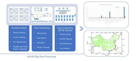
4. Supercomputing InSAR System
Time-series InSAR data processing includes more than a dozen image processing algorithms and several assistant methods. The TIF format images, obtained by Sentinel-1 satellites, are as input of the pipeline and each image has about 1.3 G bytes. In Sentinel-1 TOPS mode, we need remote sensing images of the same region in different time periods. If the surface deformation is calculated within a one-year period, the original images of each small region would have 100G bytes. Only in China there are over 350 similar regions and the original data from Sentinel-1 satellites could have as many as 33 TB to 35 TB. Moreover, the whole InSAR process will produce ten times the amount of intermediate data compared with the original. Therefore, if we want to calculate the nation-scale surface deformation of China in a short time, it is impossible only to rely on parallel algorithms and task scheduling. It is of great significance to develop a distributed system for InSAR big data processing.
Supercomputers are well known for their powerful computing power and high-performance parallel file systems, making them ideal for computation-intensive and data-intensive tasks such as numerical weather forecasting, computational chemistry, molecular modeling, astrophysical simulations, and automotive design simulations. However, there have been few applications of supercomputers for InSAR calculations. To take advantage of supercomputing, we have developed a supercomputing-InSAR system specifically designed to handle big SAR data. This platform consists of dozens of nodes dynamically allocated by the supercomputing system, and supports both single-node and multi-node operations. The high-performance parallel file system enables parallel processing of images from different orbits on the satellite.
The overall architecture of a supercomputing system is depicted in
Figure 6. Users typically log into a login node to connect to the supercomputing system and perform various operations, including configuring the environment and compiling programs. Computing nodes, which are made up of servers, are linked to one another via a network and are primarily used to carry out computational tasks. Additionally, a storage node, comprising data storage servers, is used for big data storage. The supercomputing management system uses a proprietary system to manage the computing cluster. Our supercomputing system is managed by SLURM.
Our supercomputing InSAR system is composed of four subsystems: a preprocessing subsystem, InSAR subsystem, job submission subsystem, and log analysis subsystem.
4.1. Preprocessing Subsystem
The preprocessing system is responsible for preparing the data for the InSAR processing pipeline. This includes data decompression, directory generation, and copying of DEM and track data. Additionally, the system performs environmental configuration and program compilation to ensure that the processing jobs can be executed successfully on the supercomputing platform. To prepare for big data processing on the supercomputing platform, the required image data and parameter files must be selected for unified calculation. Data preparation involves selecting the necessary compressed files from the data pool, which contains a large number of .zip files downloaded from the Sentinel-1 website, as well as preparing the corresponding DEM and orbit files. The main program is compiled into binary executable programs in advance.
Our supercomputing platform includes two main storage paths: and . is a common storage directory with ample space but relatively low reading and writing performance, and it is used primarily for storing data. In contrast, is a high-performance storage directory with limited space but strong reading and writing capabilities, and it is mainly used for data reading and writing during actual operations. Our storage strategy involves storing data initially in the directory, and then decompressing it into the corresponding directory for processing. After the calculation is complete, the final results are copied back to the directory.
All the work mentioned above is implemented through shell scripts and could be executed automatically. The whole data preprocessing process can be divided into the following steps:
Select require data from the data pool and store it in the directory.
Create a matching file structure in the directory as the one in .
Decompress the .zip files and copy their corresponding DEM and orbit files to the directory. This part will use some nodes of supercomputing system by job submission.
Configure the environment and compile the necessary third-party libraries for InSAR on the login nodes. Then, precompile the program into an executable file.
4.2. InSAR Subsystem
InSAR processing is characterized by a large volume of data and high algorithmic complexity. Therefore, load balancing, data dependency, and communication issues must be considered during actual operations. The Sentinel-1 sequential InSAR algorithms consist of multiple complex processing steps, each with a different data structure. Furthermore, there is a strict execution sequence between modules in the pipeline. The InSAR subsystem serves as the core processing section for high-performance time-series InSAR calculations, including parallel algorithms and task schedulers.
The InSAR subsystem optimizes the entire time-series InSAR pipeline to tackle computing-intensive and data-intensive problems. Parallel models improve the efficiency of algorithms and significantly reduce the time required to run the pipeline. Load balancing does not need to be considered when designing parallel models because the bursts in TOPS mode and SLC images in interference processing have the same block size. Our STAR, which is driven by the data flow model, implements data parallelization through task scheduling at a higher granularity. This further improves CPU utilization and data processing efficiency.
InSAR subsystem is the core part with many heavy computing tasks. The details are introduced in
Section 2 and
Section 3, and we will not describe it too much here.
4.3. Job Submission Subsystem
We employ the SLURM scheduling system to manage and maintain our supercomputing resources. SLURM maintains a queue of tasks to be processed and oversees overall resource utilization. It manages available computing nodes, either shared or non-shared, based on resource requirements, allowing users to execute their jobs. SLURM also allocates resources for job queues and monitors them until completion. The
Figure 7 illustrates the general workflow of our supercomputing system.
To execute a large computing task on our supercomputing system, we divide it into multiple subtasks or “jobs” at the login node. These jobs are then submitted to the job scheduling system through the job submission subsystem. The job scheduler automatically allocates resources based on the application’s requirements and releases them once the computation is complete. Therefore, the job submission subsystem is responsible for the automatic submission of all computing tasks on our supercomputing system.
Task submission can be achieved through three types of scripts: InSAR programs script, .sbatch script, and job batch submission scripts. The InSAR programs script automates the entire processing pipeline. The .sbatch script submits the computation tasks to the supercomputing system, and the SLURM management system allocates resources based on the requirements specified in the .sbatch script, such as nodes, memory, and threads. The job batch submission scripts automate the submission of .sbatch scripts to the supercomputing system.
Due to constraints of the supercomputing job scheduling system, a user is limited to a maximum of running jobs (25 jobs). Any additional submitted jobs are queued and processed after some of the running jobs are completed. To automatically submit all subtasks to the SLURM system and avoid job waiting queues, we adopt a job strategy, as shown in
Figure 8. This strategy involves submitting no more than 25 jobs (usually the maximum) and using heartbeat detection to periodically check job states. If more than 25 jobs need to be submitted, we submit the initial 25 and use heartbeat detection to determine the next set of jobs to submit. This process continues until all jobs have been submitted, ensuring a maximum of 25 running jobs on the supercomputing system without a waiting queue.
4.4. Log Analysis Subsystem
The log analysis subsystem is primarily designed to handle the log files generated by the supercomputing InSAR system. For each job, a log file with a size exceeding 300 KB is produced, and a total of 350–370 similar files are generated at national scale. Manually filtering these files to obtain the operation status of each image in each stage would be cumbersome and inefficient. Hence, the log analysis subsystem aims to extract the operational status of all images at each stage to avoid errors caused by complex manual operations.
The log analysis subsystem extracts the runtime for each phase from all log files and creates a .csv file. This file can be opened using Excel 2019 or other similar software to view a clear table that lists the runtime for all stages of each job. This functionality enables users to quickly determine if the data are correct and locate any bugs that may be present.
5. Experiments and Discussion
We use three different programming languages for various purposes in our process. The algorithms of time-series InSAR are implemented with C11/C++11 for high performance: OpenMP for parallel algorithms and MPI for distributed computing. Python 3.6 scripts generate auxiliary files between different modules for simplicity. We write shell scripts to connect all tasks and support the whole supercomputing InSAR system. By defining the relationship between tasks, as well as specifying certain parameters such as multi-look and global reference point in advance, the InSAR pipeline can automatically process data. We conduct experiments and analysis using images obtained from Sentinel-1 satellites.
5.1. Module Optimization
We tested the running time of all modules with 27 scenes of Orbit 142-1 (from July 2017 to June 2018) and provided the result for main modules before and after parallelization and optimization, operated with a server of 64 threads, 256 GB memory and 2.30 GHz Intel(R) Xeon(R) Gold 6129 CPU, as shown in
Figure 9. It should be noted that the total in this figure does not refer to the overall running time of the entire pipeline, but the sum of running time of these modules.
In
Figure 9, it is obvious for the great performance improvement that the two modules, image registration, and topography and flatten phase have been processed in parallel with 64 threads. Others have been mainly optimized in IO and memory so that the optimization result is also considerable. If all images could be calculated according to the execution order of these modules, that is, there is no pipeline parallelism, the total optimized running time is about 22 h. This result already satisfies the requirement of processing 27 scenes of a single orbit track with just one server.
This diagram clearly indicates that two programs in our process are highly demanding in terms of CPU processing time: geometric registration and calculation of the topography and flatten phase. These modules require significant processing power not only due to the complexity of their algorithms, but also because they need to be executed frequently throughout the processing flow. On the other hand, other algorithms, such as network construction and phase unwrapping, which are also highly complex but executed only once, can be accepted without parallel optimization.
5.2. Parallel Computing
5.2.1. Multi-Thread Computing
We used four scenes of Orbit-142, which included a total of 12 images captured between September and October 2018. Among these, we selected three master images, all captured during the same period but distinguishable by date and stripe. Specifically, these master images are labeled as 20180912/IW1, 20180912/IW2, and 20180912/IW3, respectively. The remaining images are considered as slave images and must undergo registration tasks with their corresponding master images. Ultimately, four SLC images were generated using TOPS mode processing for phase calculation of topography and flat-earth, labeled with the dates 20180912, 20180924, 20181006, and 20181018, respectively.
Image registration and topography and flat-earth calculation are the two major computing hotspots in the InSAR pipeline. We tested their parallel algorithms using the images mentioned above and the same operating platform as in the previous experiment. We recorded the running time of these two algorithms with different thread configuration, and the results are presented in
Table 1, where Algorithm 1 denotes the image registration algorithm and Algorithm 2 represents the flat-earth phase removal algorithm.
The impact of the number of threads on running time of both algorithms can be observed, with runtime decreasing as the threads number increases. When the thread number is set to 1, the algorithm is executed serially without any multi-thread acceleration, whereas other thread numbers indicate parallel optimization. However, the speedup ratio is non-linear, i.e., the running time is not proportional to the number of threads, but rather positively related to it within a limited number of threads. Generally, using more threads could reduce the computational burden on each thread, but too many can lead to an overall decrease in performance due to system overhead and communication between threads, compared with the speedup of configurations of 48 and 64 threads in Algorithm 1.
It is worth noting that performance can be affected by different process configurations. For instance, in the configuration where there are two processes and each has 32 threads, and there are four processes and each has 16 threads, 64 threads participate in the calculation in total. For image registration, the benefits of multiple processes are evident since burst data blocks need to be distributed to several processes. For topography and flat-earth calculation, two or four processes share the total calculation task, and there is a slight improvement in performance compared to using a direct configuration of 64 threads.
This table could be regarded as a reference for choosing an appropriate configuration of threads and processes, and other factors should be taken into consideration, such as hardware resources and actual conditions.
5.2.2. Multi-Node Computing
We explore the impact of multi-node multi-thread computing on parallel algorithms with distributed computing to choose suitable parameters for our supercomputing system. In this part, 32 scenes (Orbit 142-0) are collected from September 2018 to February 2020 as source data.
Figure 10 shows the result of operation time for TOPS mode interference processing. Similarly, the node set to 1 means it is the single-node multi-thread computing mode, and others are the multi-node multi-thread mode. The more nodes we used, the more threads involved in parallel computing, and the faster the algorithm runs.
However, it has the same problem with multi-thread computing that when more than three nodes are used for calculation, the performance does not increase linearly. The reason is that the entire process is not completely parallel, and some nodes have more computational tasks than others so that the overall performance would decrease. It is more necessary to evaluate the relationship between speedup and used computing resources. It tells us in parallel computing, more threads and nodes does not mean higher performance.
5.2.3. Parallel Strategy
In addition to several parallel hot-spot models, the whole InSAR processing system has other modules with low parallelism, i.e., the serial execution, especially the time-series processing analysis part. Parallel and serial modules together constitute the whole data processing flow. With the limitation of computing resources, we tested three orbit sets with three servers to run the pipeline. The data used comes from Orbit 142-1, 142-2 and 142-3, which contain 63, 68, and 67 images collected by satellites from 2018 to 2020, respectively. We used three computing nodes with similar performance in the supercomputing system to test the performance on three data sets, respectively.
In
Table 2, scheme 1 refers to the processing mode which calculates the three data sets of 142-1, 142-2, and 142-3 one by one with multi-thread and multi-node parallel computing, whereas scheme 2 means the mode in which three nodes compute with three data sets separately with multi-thread and single-node parallel computing. This means it is different for resources to be invested in computing.
The processing time of scheme 1 for each data set is about half of the one of scheme 2, but the total time is the sum of all processing time of three frames. Although the scheme 2’s performance for each set has declined, the total processing time is the longest runtime of three frames. Compared with the final time of the three frames, scheme 2 is half of the scheme 1. Therefore, in InSAR big data processing with limited computing resources, multi-thread and single-node process scheme might be a better choice.
5.3. Performance of STAR
In this experiment, we test the performance of our task scheduling system STAR for TOPS mode data processing.
Table 3 lists the result of TOPS mode processing with OpenMP and STAR. Sync. is synchronization and Asyn. refers to asynchronization. The main difference between them is the order of writing files and executing tasks. Impr. means percentage of performance improvement of InSAR + STAR in a Sync. or Asyn. situation over InSAR + OpenMP without task scheduling. IW in the table refers to the number of strips processed simultaneously, and InSAR means the runtime of InSAR without STAR. In general, OpenMP could be used to process multiple stripes in parallel to replace task scheduling instead. The data and operation environment are the same as the first experiment and the maximum number of parallel stripes is 12.
From the table, performance with task scheduling is significantly improved. The more strips, the more parallel pipelines, the higher the utilization of threads. In the absence of task scheduling, there is a certain gap in running time of multiple pipelines in the same loop, which leads to the running time of this loop depends on the most time-consuming one, and then the next loop is carried out. This is considered as streams synchronization. STAR breaks this synchronization mechanism. When a workflow is completed, another stream will be directly executed. No synchronization ensures worker threads are at full or near full load. When IW is set to 3, it is just possible to complete the task with four full loops without task scheduling whereas when IW is 6, it needs two full loops. The more loops, the more times it needs stream synchronization. Another factor is the order of reading/writing files and computing, i.e., Sync. and Asyn. in the table. Each thread can be executed in the order of reading files, computing, and writing files (Sync.), or one thread can read and write files, and other threads are responsible for computing (Asyn.). This leads to performance improvement. When IW is 12, there is no stream synchronization and files are written after all calculations are finished without STAR scheduler. The simultaneous operation of writing and computing determines a small improvement in the performance of STAR scheduling.
5.4. Computing in Supercomputing System
5.4.1. Data Transmission
As mentioned in
Section 4, during data preparation, various data files involved in calculation need to be transferred from common storage (
file system) to a high-performance storage (
file system). We record the transfer time of different track data between the two file systems, as shown in
Table 4.
These data are from the central region of China. The transfer speed between these two file systems can be calculated from transmission data size and time. It is not constant but is affected by the state of these two file systems.
Table 4 could be a reference for other data from other orbit.
5.4.2. Memory Usage Test
The strategy we adopt in the supercomputing system is that one frame is calculated by one node. Each frame contains many strips and the size of each stripe is about 1.2 GB. Limited by the node’s memory, there is an upper limitation on the number of stripes that can be processed at the same time.
Table 5 lists the number of stripes processed simultaneously and the peak memory that can be reached.
Since the maximum memory of each node is 256 GB, the actual available memory is about 240 GB. When the number of stripes is set to 18, the peak memory reaches about 221 GB. There is a risk that the program will crash due to insufficient memory. In a single node, we choose 15 stripes to process simultaneously for program safety.
5.4.3. Surface Deformation Map of China
The supercomputing system could support only 25 computing nodes (40 threads per node) for our large-scale time-series InSAR data processing. Due to the limited computing nodes, the multi-node computing scheme is not applied in our supercomputing InSAR system. If we insist on computing an orbit data with multi-node strategy, it will be very inefficient to process more than 11,000 scenes. Therefore, the single-node multi-thread parallel execution strategy was adopted to balance the computational burden and performance with limited kernel and memory.
To obtain the surface deformation of China within a reasonable time, we used our supercomputing InSAR system to process massive InSAR data.
Table 6 lists the total calculation time for several tracks from January to December in 2020. The total amount of processed data exceeds 400 TB including initial images and intermediate data. On average, the processing time of one frame is about 3–4 h.
Figure 11 shows another deformation map of China in 2020. We obtained the nation-wide deformation calculation result in 5 days. It is quite efficient to process massive large-scale InSAR data in a few days with only 25 computing nodes.
Figure 12 shows the surface deformation of China in 2018–2019. It is the first surface movement map of China. The volume of Sentinel-1A/B data covering the whole country from September 2018 to February 2020 we processed is more than 700 TB (33 tracks, 370 frames and 11,922 scenes). Our system processed these scenes in only 7 days.
6. Conclusions
We initially proposed multi-thread parallel time-series InSAR algorithms for Sentinel-1 data to mitigate the long runtime of high-complexity models. Our analysis focused on the sequential algorithms and data structure in different processing stages, including TOPS mode data registration, interference processing and time analysis. By identifying the independence of computation and data in these algorithms, we optimized hot-spot methods with parallel computing by performing calculations in units of image rows or columns instead of pixels. The implementation InSAR algorithms with high parallel efficiency and scalability ensures accuracy and significantly improves the performance of InSAR data processing.
In addition, we have designed an asynchronous task scheduling system based on the data flow model to further improve resource utilization in the InSAR pipeline. Utilizing the STAR parallel computing architecture, we have developed a highly efficient time-series InSAR processing platform that addresses the challenges of module dependencies and task parallelism. By configuring the thread pool appropriately, STAR architecture can execute a single pipeline or multiple pipelines simultaneously. This approach enables dynamic allocation of computing resources and efficient parallelism without the need for synchronization between pipelines.
Finally, we have developed a parallel time-series InSAR big data processing platform in a supercomputing environment to deal with large data amounts. To enhance InSAR big data processing capabilities, we depended on parallel computing based on shared memory, asynchronous task scheduling, and supercomputing job scheduling. This enabled us to achieve algorithm parallelism, task parallelism, and data batch processing. With this supercomputing InSAR system, we processed a large-scale Sentinel-1 data covering the entirety of China, completing a task that would have taken over a year in just several days. We employed this system for deformation measurements of China and acquired two large-scale deformation maps. Our system has solved the problems of high time cost and low efficiency in InSAR surface deformation measurement at a national scale, enabling us to develop large-scale geological disaster warning systems based on InSAR technology.
In the future, we will further improve performance of the algorithms by adopting a heterogeneous computing system. The main processing approach will combine distributed and single-machine processing with load balancing and fault-tolerant mechanism, enabling more efficient and intelligent computing in a large cluster environment.


