Few-Shot PolSAR Ship Detection Based on Polarimetric Features Selection and Improved Contrastive Self-Supervised Learning

Abstract

Deep learning methods have been widely studied in the field of polarimetric synthetic aperture radar (PolSAR) ship detection over the past few years. However, the backscattering of manmade targets, including ships, is sensitive to the relative geometry between target orientation and radar line of sight, which makes the diversity of polarimetric and spatial features of ships. The diversity of scattering leads to a relative increase in the scarcity of PolSAR-labeled samples, which are difficult to obtain. To solve the abovementioned issue and extract the polarimetric and spatial features of PolSAR images better, this paper proposes a few-shot PolSAR ship detection method based on the combination of constructed polarimetric input data selection and improved contrastive self-supervised learning (CSSL) pre-training. Specifically, eight polarimetric feature extraction methods are adopted to construct deep learning network input data with polarimetric features. The backbone is pre-trained with un-labeled PolSAR input data through an improved CSSL method without negative samples, which enhances the representation capability by the multi-scale feature fusion module (MFFM) and implements a regularization strategy by the mix-up auxiliary pathway (MUAP). The pre-trained backbone is applied to the downstream ship detection network; only a few labeled samples are used for fine-tuning and the construction method of polarimetric input data with the best detection effect is studied. The comparison and ablation experiment results on the self-established PolSAR ship detection dataset verify the superiority of the proposed method, especially in the case of few-shot learning.

1. Introduction

As a penetrating active sensor, synthetic aperture radar (SAR) is not limited by time or weather conditions and plays an important role in remote sensing [1]. With the development of sensor technology, SAR imaging mode has been expanded from single-polarization to full-polarization with more available scattering information, and the previous study [2] has proven that the utilization of polarimetric information can significantly improve the performance of polarimetric SAR (PolSAR) target interpretation. Ship detection has been a hot topic of research in SAR/PolSAR applications for many years. It helps to strengthen the management of maritime traffic and has a good application prospect in both civilian and military fields, such as safeguarding maritime rights and interests and improving maritime early warning capabilities.

SAR/PolSAR ship detection approaches can be classified into statistical characteristic-based, polarimetric feature-based, and spatial feature-based methods. The statistical characteristic-based method is based on the assumption that the sea background is relatively dark to ship targets, therefore, ships can be detected by modeling the sea clutter through statistical analysis and searching for outliers. The constant false alarm rate (CFAR) and its variants [3] belong to this kind of method. Gao et al. [4,5,6] studied the statistical modeling and parameter estimation of clutter for ship detection. Tao et al. [7] proposed an adaptive truncation method to estimate the parameter of the statistical model, and Liu et al. [8] extended it to PolSAR images. The polarimetric feature-based method distinguishes the ship from the sea clutter with the help of polarimetric features. Ringrose et al. [9] applied the polarimetric features obtained by Cameron decomposition for ship detection in the ocean. Touzi et al. [10] used the polarization entropy, eigenvalue and average of scattering angles decomposed from the polarimetric covariance matrix to detect ships. Chen et al. [11] proposed polarization cross-entropy and proved the effectiveness of this feature in ship detection on AIRSAR data. Sugimoto et al. [12] utilized the decomposition of the four-component model proposed by Yamaguchi for ship detection. Yang et al. [13,14] proposed the generalized optimization of polarimetric contrast enhancement (GOPCE) to detect ships. Gao et al. [15] combined polarization entropy and backscattered energy to detect ships in PolSAR images, showing the advantages of feature fusion in the energy domain and the polarization domain. Xu et al. [16] proposed a new parameter, surface scanning randomness (SSR), to enhance the contrast between wake and sea. The potential ship wakes can be extracted through the digital axoids transform of SSR, and the ships are detected indirectly by detecting ship wakes. The spatial feature-based method uses artificially designed or automatically learned features extracted in the spatial domain for discriminating ships from sea clutter. Early traditional methods rely on features and detectors designed by experts. Kaplan et al. [17] proposed an extended fractal feature that is sensitive to the target scale and can achieve fast detection. Grandi et al. [18] used the wavelet features for detecting targets in PolSAR images, which explained the dependence of texture measurement on the polarization state. In addition, deep learning is also a method based on spatial features.

At present, deep learning has become the mainstream method in ship detection for its excellent spatial feature extraction ability. Li et al. [19] used the Faster R-CNN architecture, and Lin et al. [20] improved the performance of SAR ship detection by using the squeeze and excitation mechanisms. Wang et al. [21] applied a single-shot multi-box detector (SSD) to target detection in SAR images and boosted the detection precision with data augmentation and transfer learning. Zhang et al. [22] proposed a high-speed SAR ship detection approach by improving you only look once version 3 (YOLOv3) and realized fast detection on a public SAR ship detection dataset (SSDD) by simplifying the network structure. Zhu et al. [23] took fully convolutional one-stage object detection (FCOS) as the baseline and re-designed its feature extraction, classification and regression to detect dim and small ships in large-scale SAR images with higher accuracy. Similarly, they introduced the adaptive training sample selection (ATSS) version of FCOS (FCOS and ATSS) as the baseline and improved it for ship detection in SAR images [24]. Most of the current deep learning-based SAR ship detection research focuses on single-polarization SAR images, which mainly extract the spatial features of SAR ships. However, the studies with regard to deep learning-based ship detection in PolSAR images are few, and the polarimetric features are also not well utilized in these studies. In summary, it is meaningful to explore a PolSAR ship detection method utilizing neural networks to process the polarimetric feature, and which kind of polarimetric feature is more suitable for the network is also worth investigating. How to better extract polarimetric and spatial features in the process of PolSAR ship detection based on deep learning is an urgent problem to be solved, and so this paper aims to put forward a PolSAR ship detection method by better making use of the polarimetric and spatial information.

Another issue that needs to be addressed for PolSAR ship detection based on deep learning is the few-shot problem because of the scarce data. The acquisition of labeled PolSAR ship is not as simple as that of natural images, and the following characteristics of PolSAR targets exacerbate the issue. The scattering characteristic of a PolSAR target is sensitive to the relative geometric relation between target orientation and radar line of sight [25,26]. For the same target, when its orientation relative to the radar line of sight is different, its polarimetric features could be significantly different. For different targets, they may also exhibit very similar polarimetric scattering features under specific orientations. The same issue occurs for the spatial features. To sum up, the scattering diversity of PolSAR targets presents a great challenge for target detection in PolSAR images, especially when there are only a few training samples, since it is extremely hard to learn the effective discriminating features with quite limited samples for the data-driven method. What is more, azimuth ambiguity, reef influence, and high sea conditions also increase the difficulty of PolSAR ship detection with only a few labeled training samples, since the model is prone to overfit the training data and thus lacks generalization ability to the un-seen data. Under the few-shot case, interference objects such as offshore drilling platforms, reefs, lighthouses, buoys, etc. are probably wrongly recognized as ships, and some ships could go un-detected due to the complex background. Few-shot learning in SAR target interpretation has attracted lots of attention. Rostami et al. [27,28] borrowed the knowledge from the panchromatic remote sensing image classification task to the SAR image classification task through transfer learning to mitigate the few-shot issue of SAR data, and the distribution difference of features in the panchromatic domain and the SAR domain is minimized through domain adaptation. Wang et al. [29] used a hybrid inference network combining inductive inference and transductive inference to predict the class of the feature space mapped by the embedded network, and completed the classification of few-shot SAR images by enhancing the interclass separability in the embedding space with a novel loss function named enhanced hybrid loss. Fu et al. [30] proposed a meta-learning framework consisting of a meta-learner and a basic learner that can learn a good initialization as well as a proper update strategy and implement fast adaptation with a few training images on new tasks after training. Each of the aforementioned few-shot learning methods presents certain limitations. Transfer learning typically involves a more intricate design process, necessitating the meticulous selection of transfer schemes that are specifically tailored to the particular problem at hand [31]. The transductive inference method is challenging to integrate into various target detection frameworks, and the meta-learning approach relies on a sequence of similar tasks. Therefore, it is imperative to explore alternative approaches to mitigate these shortcomings. Recently, contrastive self-supervised learning (CSSL) has achieved impressive results for few-shot learning in the field of computer vision, which learns general representations from massive un-labeled data, and can be used in downstream tasks with only a few samples to finetune the pre-trained model. The basic principle of CSSL is to learn the underlying image representations by grouping similar samples (positive pairs) together and pushing diverse samples (negative pairs) away from each other. The representative methods include MOCO [32] and SimCLR [33]. There are other kinds of CSSL methods that only make use of positive pairs, such as BYOL [34] and SimSiam [35]. The reason for taking out negative pairs is that the samples in a negative pair could be very similar, making the training model hard to converge. Another advantage of the CSSL method without negative pairs is its training efficiency. By only processing the positive pairs, many resource consumptions can be saved. The research on the application of CSSL in remote sensing is at an elementary stage [36], and most current studies are conducted for classification tasks. Similarly, Zhang et al. [37] proposed a PolSAR-tailored contrastive learning network (PCLNet), which learns useful representations from un-labeled PolSAR data through an un-supervised pre-training phase. The acquired representations are transferred to the downstream task to achieve few-shot PolSAR classification. Yang et al. [38] proposed a coarse-to-fine CSSL framework, which made the global and local features learned respectively through the pre-training of two stages and realized the land-cover classification in SAR images with limited labeled data. How to apply CSSL on the PolSAR ship detection task for coping with the few-shot issue needs to be investigated, and this is another purpose of this study.

In this paper, we propose a few-shot PolSAR ship detection method based on polarimetric feature selection and improved contrastive self-supervised learning. Firstly, eight polarimetric features obtained via various polarization decompositions, polarimetric coherence, and speckle filtering are taken into consideration to serve as the input of the network. Then, taking SimSiam as the baseline, an improved CSSL method with a multi-scale feature fusion module (MFFM) and mix-up auxiliary pathway (MUAP) is proposed to learn the effective representation of PolSAR data. Specifically speaking, MFFM is proposed to replace the common convolution layer in the residual block. The input feature map of MFFM is divided into several groups along the channel dimension. These groups are individually passed through dilated convolution layers with various dilation rates, so multi-scale feature maps can be obtained by the above-mentioned process. The multi-scale feature maps are merged through the concatenation operation along the channel dimension to get the output feature map of MFFM. MFFM can enhance the representation ability of the network by merging multi-scale features and enlarging the receptive field through a dilated convolution operation. MUAP takes the linear combination of the two inputs of the vanilla CSSL as its input and encourages the model to behave linearly in-between training samples. MUAP enriches the diversity of the input and promotes the robustness of the representations learned by CSSL. Finally, the model pre-trained from the improved CSSL is taken as the feature extractor of the Faster R-CNN detector and finetuned with a few PolSAR ships. The main contributions of this paper are summarized as follows:

(1)

To our best knowledge, this is the first study introducing self-supervised learning into PolSAR ship detection. An obvious performance gain is achieved by CSSL, especially when the training samples are few.

(2)

We propose an improved CSSL method with two new modules. The multi-scale feature fusion module enhances the representation capability via multi-scale feature fusion, and the mix-up auxiliary pathway improves the robustness of the features through a mix-up regularization strategy.

(3)

Eight various polarimetric features are extracted by different polarization decomposition, polarimetric coherence, and speckle filtering, and the effect of them with the proposed improved CSSL method is compared to explore which polarimetric feature is more suitable to our contrastive learning framework.

(4)

Comprehensive experiments are conducted to validate the effectiveness of the proposed method, and the results indicate that our method achieves state-of-the-art PolSAR ship detection performance in comparison with recent studies, especially under the few-shot situation. In addition, our method also mitigates the shortcomings of other few-shot learning methods.

The remainder of this paper is organized as follows: The proposed method is detailed in Section 2, followed by experimental results in Section 3. Some discussions are presented in Section 4, and Section 5 concludes the paper.

2. Methods

In this paper, a few-shot PolSAR ship detection method based on polarimetric feature selection and improved contrastive self-supervised learning is proposed. The overall architecture of this method is given in Figure 1. Firstly, polarimetric features are extracted from the input PolSAR image, and the details will be presented in Section 2.1. The effect of eight different kinds of polarimetric features obtained via various polarization decomposition, polarimetric coherence, and speckle filtering is investigated in the experiment parts and sheds light on how to select the polarimetric feature for the PolSAR ship detection task. Secondly, the above polarimetric features obtained by different types of polarization decomposition algorithms are fed to an improved CSSL network in the form of multi-channel images, respectively, and we use this method to pre-train the superior feature extraction backbone network. The improved CSSL network consists of two branches: the contrastive branch and the mixed branch. The contrastive branch is based on the SimSiam network [35], which is composed of two encoders and a predictor. For better feature extraction, we designed a multi-scale feature fusion module (MFFM) to optimize the backbone of the encoder (e.g., ResNet [39]). To go further, we proposed the mixed branch, which is called mix-up auxiliary pathway (MUAP) here and is built up as a regularization term. The two branches of the network share the weights. As a result of these operations, the backbone network’s ability to learn polarimetric and spatial features has been enhanced. All details will be discussed at length in Section 2.2. Finally, the feature extraction backbone pre-trained by the improved CSSL method is applied to the deep learning ship detection network (Faster R-CNN [40]). We then fine-tuned the detection network using only a few labeled ship samples and found that the network achieved excellent ship detection results. This part will be discussed thoroughly in Section 2.3.

2.1. Input Data Construction by Polarimetric Feature Extraction

PolSAR can obtain fully polarimetric information about the target by sending and receiving electromagnetic waves with orthogonal polarization states. By modeling and analyzing the electromagnetic scattering characteristics of the target, various physical parameters of the target can be more accurately retrieved. In this paper, we constructed the data with various practical physical meanings through polarization decomposition, polarimetric coherence and speckle filtering methods, and then fed these data to the subsequent ship detection network. The eight polarimetric feature extraction methods that we use in the construction of the input data phase are Pauli decomposition [41], Cloude decomposition [42], Freeman decomposition [43], Yamaguchi decomposition [44], Cui decomposition [45], polarimetric coherence [46], Refined Lee filter [47] and Adaptive filter [48]. The details of these polarimetric feature extraction methods are described as follows.

2.1.1. Polarization Decomposition

Polarization decomposition theory has been developed continuously in recent years, which is an effective tool to interpret the target scattering mechanism. It decomposes the scattering matrix or covariance matrix into a combination of basic components according to different physical scattering types and can be effectively applied to ship detection in PolSAR images [49]. Polarization decomposition can be divided into coherent decomposition and incoherent decomposition.

Coherent decomposition is based on the polarimetric scattering matrix. As a representative method of coherent decomposition, the Pauli decomposition [41] method is adopted as one of the input data construction methods. Pauli decomposition represents the polarimetric scattering matrix $S$ as the weighted sum of Pauli-basis. The $S$ matrix is represented as:

$$S=\left[\begin{array}{cc}{S}_{HH}& S_{HV}\\ S_{VH}& S_{VV}\end{array}\right]=a\left[S_a\right]+b\left[S_b\right]+c\left[S_c\right]+d\left[S_d\right],$$

(1)

where $a$, $b$, $c$ and $d$ are complex values, representing the weight of each basic scattering matrix. From the scattering vector $k$ under Pauli-basis, which becomes:

$$k=\frac{1}{\sqrt{2}}{\left[\begin{array}{cccc}{S}_{HH}+S_{VV}& S_{HH}-S_{VV}& S_{HV}+S_{VH}& i\left(S_{HV}-S_{VH}\right)\end{array}\right]}^T,$$

(2)

where ${\left(\cdot \right)}^T$ means the transpose. It can be obtained that the calculation method of $a$, $b$, $c$, $d$ as:

$$\begin{array}{ll}a=\frac{1}{\sqrt{2}}\left(S_{HH}+S_{VV}\right),& b=\frac{1}{\sqrt{2}}\left(S_{HH}-S_{VV}\right)\\ c=\frac{1}{\sqrt{2}}\left(S_{HV}+S_{VH}\right),& d=\frac{1}{\sqrt{2}}\left(i\left(S_{VH}-S_{HV}\right)\right)\end{array}.$$

(3)

${\left|a\right|}^2$, ${\left|b\right|}^2$ and ${\left|c\right|}^2$ can respectively construct single channel input data with polarimetric features. ${\left|a\right|}^2$ represents odd-bounce scattering energy, ${\left|b\right|}^2$ represents 0° dihedral angle scattering energy, and ${\left|c\right|}^2$ represents 45° dihedral angle scattering energy.

Incoherent decomposition is based on the polarimetric coherence matrix and the polarimetric covariance matrix, which includes polarimetric target decomposition based on eigenvalues and polarimetric target decomposition based on scattering models. The former refers to the eigenvalue decomposition of the polarimetric coherence matrix, and its eigenvalues and eigenvectors represent various physical meanings. As a representative method of eigenvalue decomposition, Cloude decomposition [42] is adopted to construct input data, and its expression is:

$$T={\displaystyle \sum _{i=1}^3{\lambda }_i}{u}_i{u}_i^H,$$

(4)

where ${\lambda }_i$ is the eigenvalue of the polarimetric coherence matrix $T$, $u_i$ is the eigenvector of $T$. $u_i$ can be written as:

$$u_i={[\cos {\alpha }_i\hspace{1em}\sin {\alpha }_i\cos {\beta }_i{e}^{j{\delta }_i}\hspace{1em}\sin {\alpha }_i\cos {\beta }_i{e}^{j{\gamma }_i}]}^T,$$

(5)

where angle ${\alpha }_i$ represents the scattering type of the target, $0\le {\alpha }_i\le 90°$. Angle ${\beta }_i$ represents the orientation angle of the target, $-180°\le {\beta }_i\le 180°$. Angles ${\delta }_i$ and ${\gamma }_i$ represent the phase angle of the target. $T$ can be obtained by:

$$T=〈k_p{k}_p^H〉=\left[\begin{array}{ccc}{T}_{11}& T_{12}& T_{13}\\ T_{21}& T_{22}& T_{23}\\ T_{31}& T_{32}& T_{33}\end{array}\right],$$

(6)

where $k_p$ is Pauli scattering vector, the superscript H represents the conjugate transpose operation, and $〈\cdot 〉$ means multi-look average processing. $k_p$ is represented as:

$$k_p=\frac{1}{\sqrt{2}}\left[\begin{array}{ccc}{S}_{HH}+S_{VV}& S_{HH}-S_{VV}& 2S_{HV}\end{array}\right].$$

(7)

The derived polarimetric features include the polarization entropy $H$, the average of scattering angles $\overline{\alpha }$, and the Polarization anti-entropy $A$. $H$ can be formulated as:

$$H=-{\displaystyle \sum _{i=1}^3{p}_i}{\log }_3\left(p_i\right),p_i=\frac{{\lambda }_i}{{\displaystyle \sum _{k=1}^3{\lambda }_k}}.$$

(8)

$H$ describes the statistical randomness of different scatterers in a pixel, and ranges from 0 to 1. $\overline{\alpha }$ is represented as:

$$\overline{\alpha }={\displaystyle \sum _{i=1}^3{p}_i}{\alpha }_i,$$

(9)

when $\overline{\alpha }\to 0$, it corresponds to the surface scattering mechanism; when $\overline{\alpha }\to \frac{\pi }{4}$, it corresponds to the volume scattering mechanism; and when $\overline{\alpha }\to \frac{\pi }{2}$, it corresponds to the double bounce scattering mechanism. $A$ can be written as:

$$A=\frac{{\lambda }_2-{\lambda }_3}{{\lambda }_2+{\lambda }_3}, {\lambda }_1\ge {\lambda }_2\ge {\lambda }_3>0,$$

(10)

$A$ mainly investigates the relative size between two smaller eigenvalue parameters. In addition, we add scattering power SPAN on the basis of Cloude decomposition to construct input data, which is defined as:

$$SPAN={\left|S_{HH}\right|}^2+{\left|S_{HV}\right|}^2+{\left|S_{VH}\right|}^2+{\left|S_{VV}\right|}^2.$$

(11)

Polarization decomposition based on scattering models aims to decompose the scattering mechanism of the target into a combination of basic scattering components such as double-bounce scattering, surface scattering, volume scattering and helix scattering. The scattering mechanism of the target is interpreted by analyzing the energy and other parameters of the basic scattering components. Freeman decomposition [43] and Yamaguchi decomposition [44] are adopted as polarization decompositions based on scattering models to construct input data. Freeman decomposition decomposes the polarimetric covariance matrix into surface scattering, double-bounce scattering, and volume scattering, which can be formulated as:

$$C=f_s{C}_s+f_d{C}_d+f_v{C}_v,$$

(12)

where $C_s$, $C_d$ and $C_v$ denote the surface scattering model, the double-bounce scattering model, and the volume scattering model, respectively, and $f_s$, $f_d$, $f_v$ are the corresponding model coefficients. The polarimetric covariance matrix $C$ can be obtained by:

$$C=\left[\begin{array}{ccc}〈{\left|S_{HH}\right|}^2〉& \sqrt{2}〈S_{HH}{S}_{HV}^{\ast }〉& 〈S_{HH}{S}_{VV}^{\ast }〉\\ \sqrt{2}〈S_{HV}{S}_{HH}^{\ast }〉& 2〈{\left|S_{HV}\right|}^2〉& \sqrt{2}〈S_{HV}{S}_{VV}^{\ast }〉\\ 〈S_{VV}{S}_{HH}^{\ast }〉& \sqrt{2}〈S_{VV}{S}_{HV}^{\ast }〉& 〈{\left|S_{VV}\right|}^2〉\end{array}\right].$$

(13)

The three scattering models can be expressed as follows:

$$C_s=\left[\begin{array}{ccc}{\left|\beta \right|}^2& 0& \beta \\ 0& 0& 0\\ {\beta }^{\ast }& 0& 1\end{array}\right],\hspace{1em}{C}_d=\left[\begin{array}{ccc}{\left|\alpha \right|}^2& 0& \alpha \\ 0& 0& 0\\ {\alpha }^{\ast }& 0& 1\end{array}\right],\hspace{1em}{C}_v=\left[\begin{array}{ccc}1& 0& 1/3\\ 0& 2/3& 0\\ 1/3& 0& 1\end{array}\right],$$

(14)

where $\alpha$ is a complex number and $\beta$ is a real number. Substitute Equation (14) into Equation (12) to obtain that:

$$\begin{array}{l}〈{\left|S_{HH}\right|}^2〉=f_s{\left|\beta \right|}^2+f_d{\left|\alpha \right|}^2+f_v\\ 〈{\left|S_{VV}\right|}^2〉=f_s+f_d+f_v\\ 〈S_{HH}{S}_{VV}^{\ast }〉=f_s\beta +f_d\alpha +f_v/3\\ 〈{\left|S_{HV}\right|}^2〉=f_v/3\end{array},$$

(15)

and this model gives us four equations with five un-known parameters. Freeman made assumptions about $\alpha$ and $\beta$. If $\mathrm{Re}\left\{〈S_{HH}{S}_{VV}^{\ast }〉\right\}$ is positive, fix $\alpha =-1$. If $\mathrm{Re}\left\{〈S_{HH}{S}_{VV}^{\ast }〉\right\}$ is negative, fix $\beta =1$. Then, the contribution of each scattering mechanism to the SPAN are:

$$\begin{array}{l}{P}_s=f_s\left(1+{\left|\beta \right|}^2\right)\\ P_d=f_d\left(1+{\left|\alpha \right|}^2\right)\\ P_v=8f_v/3\end{array},$$

(16)

where $P_s$, $P_d$ and $P_v$ denote the scattering power of the surface scattering model, the double-bounce scattering model, and the volume scattering model, respectively.

Yamaguchi decomposition extends Freeman decomposition and adds the helix scattering component. Cui decomposition [45] is a hybrid decomposition method based on both eigenvalues and scattering models, which is also adopted to construct input data. This method makes the polarimetric coherence matrix $T$ completely decomposed into three components contributed by volume scattering and two single scatterers. Under this scheme, solving for the volumetric scattering power amounts to a generalized eigendecomposition problem, and the nonnegative power constraint uniquely determines the minimum eigenvalue as the volume scattering power. Furthermore, both eigendecomposition and model fitting can discriminate the remaining components.

2.1.2. Polarimetric Coherence

The coherence values between different polarization channels in PolSAR data contain rich target information [46]. For two polarization channels $S_{HH}$ and $S_{HV}$, the polarimetric coherence can be written as:

$$R=〈S_{HH}{S}_{HV}^{\ast }〉,$$

(17)

where $S_{HV}^{\ast }$ is the conjugate of $S_{HV}$, $〈\cdot 〉$ means multi-look average processing, and R is generally a complex number. In order to make the coherence between different objects comparative, we normalize R by the magnitude to obtain the normalized coherence $\rho$. For example, the normalized coherence ${\rho }_{HHHV}$ between $S_{HH}$ and $S_{HV}$ is defined as:

$${\rho }_{HHHV}=\frac{\left|〈S_{HH}{S}_{HV}^{\ast }〉\right|}{\sqrt{〈{\left|S_{HH}\right|}^2〉〈{\left|S_{HV}\right|}^2〉}}.$$

(18)

Other normalized coherences are similarly defined.

2.1.3. Speckle Filtering

When the coherent electromagnetic waves emitted by PolSAR irradiate the surface of an object, if the echo phases are consistent, then a strong signal is received; if the echo phases are inconsistent, then a weak signal is received. Therefore, the echo will have a large random fluctuation, resulting in many similar granular spots on the image, which is called a speckle noise [50]. Speckle noise is an inherent defect of all imaging systems based on the principle of coherence, such as SAR, sonar, laser, etc. It is a system noise and cannot be avoided. Through speckle filtering, the spatial features of the target can be improved, but in general, the polarimetric features will suffer a certain loss after the filtering. In this paper, based on Pauli decomposition, the input data are constructed by the Refined Lee filter [47] and the Adaptive filter [48], respectively.

The Refined Lee filter uses edge-aligned non-square windows and minimum mean square error filtering. A group of edge detection templates is used to find homogeneous regions, and Lee filtering is performed in this region. Refined Lee filter can preserve the texture features of edges, but since it uses the span value to determine homogeneous regions, which does not contain sufficient pixel scattering information, the dominant scattering mechanism of each pixel is not maintained by the Refined Lee filter. The Adaptive filter is an adaptive speckle filtering method based on line edge detector and polarization homogeneity measurement. Small, non-square windows are selected for heterogeneous areas to maintain details, and large square windows are selected for homogeneous areas to filter speckle noise as much as possible.

2.2. Pre-Training of Feature Extraction Network Based on Improved Contrastive Learning

In order to enhance the feature extraction ability of the backbone and make the Faster R-CNN network have better generalization ability in the few-shot PolSAR ship detection task, an improved CSSL method based on SimSiam [35] is proposed to pre-train the backbone. The backbone plays an important role in feature extraction, and various networks can be adopted as the backbone. In this paper, the ResNet [39] serves as the backbone network to extract image representation vectors. We introduce atrous convolution [51] to build a multi-scale feature fusion module (MFFM), which optimizes the backbone so that the backbone has multi-scale feature extraction capability for ship targets of different sizes. The architecture of MFFM will be designed in Section 2.2.1. As shown in Figure 2, the proposed pre-training network consists of two branches. One is the contrastive branch, which will be detailed in Section 2.2.2. The other is the mix branch, which is referred to as the mix-up auxiliary pathway (MUAP), which has the same composition and parameters as the contrastive branch. MUAP will be described in Section 2.2.3. The final total loss of the whole network is the weighted sum of the contrastive branch loss and the mix branch loss, which is written as:

$$L_{final}=\mu L_{con}+(1-\mu )L_{mix}.$$

(19)

2.2.1. Multi-Scale Feature Fusion Module

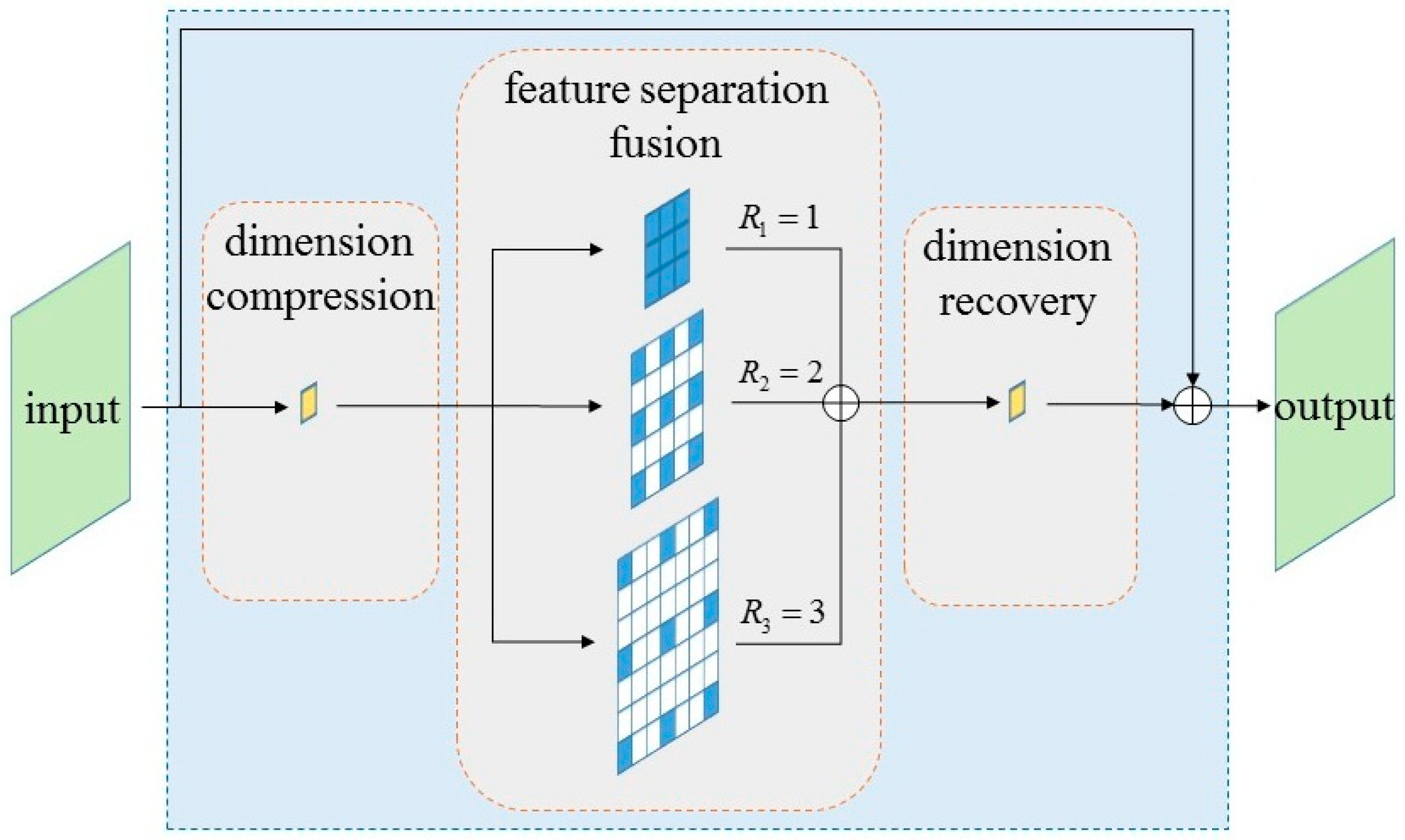
The structure of the MFFM is shown in Figure 3. Specifically, the last residual unit module at the end of the backbone is modified as a MFFM which contains two 1 × 1 convolutional layers and an atrous convolution block, and it is similar to the bottleneck block of the ResNet. Two 1 × 1 convolutional layers are used for compression and recovery of feature dimensions, respectively. The atrous convolution block consists of three atrous convolution layers with different atrous rates $R_1$ = 1, $R_2$ = 2, and $R_3$ = 3 and the same kernel size 3 × 3. The diversity of the atrous rate can ensure multi-scale feature extraction ability, and the choice of three is due to the corresponding constraint relationship between the expanded receptive field and the size of the feature map. Then, after each atrous convolution layer, the batch normalization layer is tightly added, followed by the ReLU layer to ensure the nonlinear mapping of the network. The sum function is adopted for fusing all branches, and the original feature map is merged into the final representation through the residual connection.

2.2.2. Contrastive Learning Framework

For the contrastive branch, two randomly augmented views, $x_1$ and $x_2$, from the un-labeled sample $x$ of the constructed multi-channel images containing polarimetric features are used as the input. The image augmentation methods include amplitude distortion (brightness and contrast), Gaussian blur, and rotation. These two views are processed by an encoder network $f$ to get $z_1$ and $z_2$. The encoder $f$ shares weights between the two views. In order to map the output of the encoder to the space of measuring distance, $z_1$ is output to $p_1$ through a prediction multi-layer perceptron (MLP) head [34].The prediction head, denoted as $h$, transforms the output of one view and matches it with the other view. Denoting the two output vectors as $p_1=h\left(f\left(x_1\right)\right)$ and $z_2=f\left(x_2\right)$, we minimize their negative cosine similarity $D$ as:

$$D\left(p_1,z_2\right)=-\frac{p_1}{{‖p_1‖}_2}\cdot \frac{z_2}{{‖z_2‖}_2},$$

(20)

where ${‖\cdot ‖}_2$ is ${𝓁}_2$-norm. After exchanging and separately feeding the two randomly augmented views $x_2$ and $x_1$ to get $p_2$ and $z_1$, following [34], a symmetrized loss is defined as:

$$L=\frac{1}{2}D\left(p_1,z_2\right)+\frac{1}{2}D\left(p_2,z_1\right).$$

(21)

The above equation gives the loss of one image, and the total loss is averaged over all samples.

A crucial operation for the framework is the stop-gradient operation (Figure 2), consequently the first term of the above loss should be modified as:

$$D\left(p_1,\mathrm{stopgrad}\left(z_2\right)\right).$$

(22)

In this term, $z_2$ is treated as a constant and the gradient does not flow back to the encoder network. The final loss function of contrastive branch is re-written as:

$$L_{con}=\frac{1}{2}D\left(p_1,\mathrm{stopgrad}\left(z_2\right)\right)+\frac{1}{2}D\left(p_2,\mathrm{stopgrad}\left(z_1\right)\right).$$

(23)

The encoder network on $x_2$ receives gradients from $p_1$ and no gradients from $z_2$ in the first term, but it receives gradients from $p_2$ and no gradients from $z_1$ in the second term (and vice versa for $x_1$).

2.2.3. Mix-Up Auxiliary Pathway

For the mix branch, a linear mixed view $x_m$ of the augmented views $x_1$ and $x_2$ is used as the input. Mix-up [52], as a method of data enhancement, is an effective regularization strategy, which improves the generalization ability of the model. $x_m$ is defined as:

$$x_m=\lambda x_1+(1-\lambda )x_2,$$

(24)

where $\lambda ~Beta(\alpha ,\alpha )$ is a mixing coefficient sampled from the beta distribution. The mixed view $x_m$ is fed to the mix branch which is referred to as the mix-up auxiliary pathway (MUAP), and MUAP takes the same composition and parameters as the contrastive branch. This process makes the model as close to the linear function as possible and enriches the latent representation in pre-training network [53].

Through the mix branch, an output feature vector $p_m=h(f\left(x_m\right))$ is obtained. In order to contrast the most discriminate representation, we introduce another feature vector $z_m$ which is obtained by computing the element-wise maximum among $z_1$ and $z_2$, which is formulated as:

$$z_r=\left[z_r^1,\cdots ,z_r^n\right]=\left[\max \left(z_1^1,z_2^1\right),\cdots ,\max \left(z_1^n,z_2^n\right)\right].$$

(25)

The loss of the mix branch is calculated by:

$$L_{mix}=D\left(p_m,\mathrm{stopgrad}\left(z_r\right)\right).$$

(26)

2.3. Few-Shot PolSAR Ship Detection

The classic Faster R-CNN [40] is applied as the ship detector, which uses region proposal network (RPN) to generate multiple regions that may contain targets, and then classifies and regresses each region. The pre-trained feature extraction backbone by the proposed improved CSSL method is plugged into Faster R-CNN instead of training from scratch. Only a few labeled ship samples are used to fine tune the Faster R-CNN network and few-shot PolSAR ship detection task is realized through this scheme.

Figure 4 illustrates the detection pipeline. The input PolSAR ship image is firstly fed into the pre-trained backbone to extract the feature maps. Then, the region proposal network (RPN) of Faster R-CNN is responsible for generating multiple regions that may contain targets. Next, for each candidate region (also called as anchor), the network will compute the loss for training and output whether it contains a target, and the target’s refined location during the inference stage.

The RPN loss function is defined as:

$$L\left(\left\{p_i\right\},\left\{t_i\right\}\right)=\frac{1}{N_{cls}}{\displaystyle \sum _i{L}_{cls}\left(p_i,p_i^{\ast }\right)}+\lambda \frac{1}{N_{reg}}{\displaystyle \sum _i{p}_i^{\ast }{L}_{reg}\left(t_i,t_i^{\ast }\right)},$$

(27)

where $L_{cls}$ is the classification loss which is used to classify whether candidate regions belong to targets or backgrounds, and $L_{reg}$ denotes the regression loss which is used to refine the locations of targets. The $L_{reg}$ is written as:

$$\begin{array}{l}{L}_{reg}\left(t_i,t_i^{\ast }\right)={\displaystyle \sum _{i\in \left\{x,y,w,h\right\}}Smooth}{L}_1(t_i-t_i^{\ast })\\ Smooth{L}_1(x)=\left\{\begin{array}{cc}0.5x^2& if\left|x\right|<1\\ \left|x\right|-0.5& otherwise\end{array}\right.\end{array}.$$

(28)

1.

The meaning of parameters in the above two equations are given as follows:

• $p_i$ represents the probability of the $i$th anchor of the network prediction is a target, and $p_i^{\ast }$ represents the corresponding ground truth;
• $t_i$ represents the offset of the prediction box, and $t_i^{\ast }$ represents the corresponding ground truth;
• $N_{cls}$ is the size of mini-batch, $N_{reg}$ is the number of anchors, and $\lambda$ is used to balance the two losses.

2.

The parameters of anchor regression are defined as follows:

$$t_x=\frac{x-x_a}{w_a}, t_y=\frac{y-y_a}{h_a}, t_w=\log \left(\frac{w}{w_a}\right), t_h=\log \left(\frac{h}{h_a}\right),$$

(29)

where $x_a$, $y_a$, $w_a$ and $h_a$ are the coordinates of the anchor’s center point, width and height, and $t_x$, $t_y$, $t_w$ and $t_h$ are the offsets predicted by the regression. The modified anchor coordinates are calculated by the above equation.

3. Experimental Results

In this section, comprehensive experiments are conducted to validate the effectiveness of the proposed method. Specifically speaking, (1) the effect of input data with polarimetric features constructed by different type of polarimetric feature extraction algorithms are explored, (2) the soundness of the proposed improved CSSL method will be validated by comparing the detection performance of the network with the pre-trained backbone and the network trained from scratch, and (3) the impact of the structure of backbone on the detection accuracy is also discussed.

3.1. Data Description

We use 26 fully PolSAR images from Chinese GF-3 satellite at different locations for experiments, of which 8 PolSAR images are used for the backbone pre-training and 18 PolSAR images are used for the ship detection network training and detection. GF-3 satellite is one of the civilian space-borne SAR systems with 12 imaging modes, such as stripmap, spotlight, scanSAR and so on, and the resolution can reach up to 1 m [54]. The used 26 fully PolSAR images are obtained by the imaging mode of QPSI, and has the spatial resolution of 8 m and the observation swath of 30 km. The product level is L1A, which provides the complex data of images with HH, HV, VH and VV polarizations.

The experiment includes backbone pre-training based on the improved CSSL mthod and fine-tuning based on Faster R-CNN target detection network.

In the improved CSSL pre-training stage, eight GF-3 PolSAR images containing multiple scenes (ocean, port, hill, city, etc.) are selected for making self-supervised PolSAR datasets to train the feature extraction backbone network. These 8 GF-3 PolSAR images range from 3891 pixels to 7834 pixels in width and 5938 pixels to 8072 pixels in height. In order to make full use of the input images with various polarimetric features, according to the 8 polarimetric feature extraction methods, the channel superposition method is used to fuse the images extracted by each method, and a total of 8 × 8 fused images are obtained where 8 is the number of original PolSAR images. Then we cut the 8 original images into small images which are 40 pixels by 40 pixels. After the cutting operation, a total of 225,313 un-labeled PolSAR small size images are obtained by each polarimetric feature extraction method. These images form the un-supervised PolSAR dataset and are used to pre-train the feature extraction backbone network by the improved CSSL method.

In the Faster R-CNN network training stage, 18 PolSAR images with ships in open sea, nearshore and in harbor scenario near the area of Shanghai and Hong Kong are taken to construct the training and the test datasets for ship detection. The datasets also adopts the channel superposition method to obtain 8 × 18 fused images with 8 polarimetric feature extraction methods on the 18 original PolSAR images, and the fused images are cut into multiple 512 pixels × 512 pixels small size images. Furthermore, in order to reduce the useless information in the dataset and improve the learning effect, small size images are filtered based on whether they contain complete ship targets. Then, each polarimetric feature extraction method obtained 283 labeled small size images containing ship targets. Among them, 198 images (70% of the total number of images) are set as the training set and 89 images (30% of the total number of images) are set as the test set. The open source annotation tool Labelme is used for labeling the ships in the COCO format.

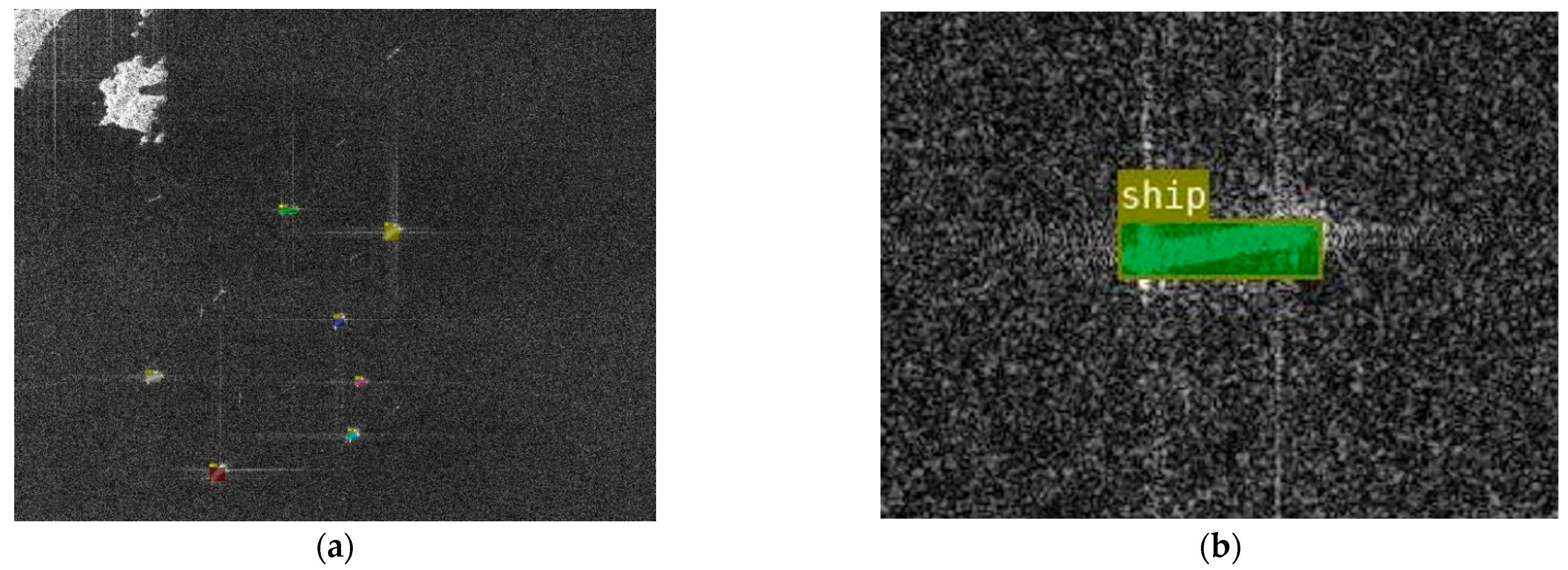
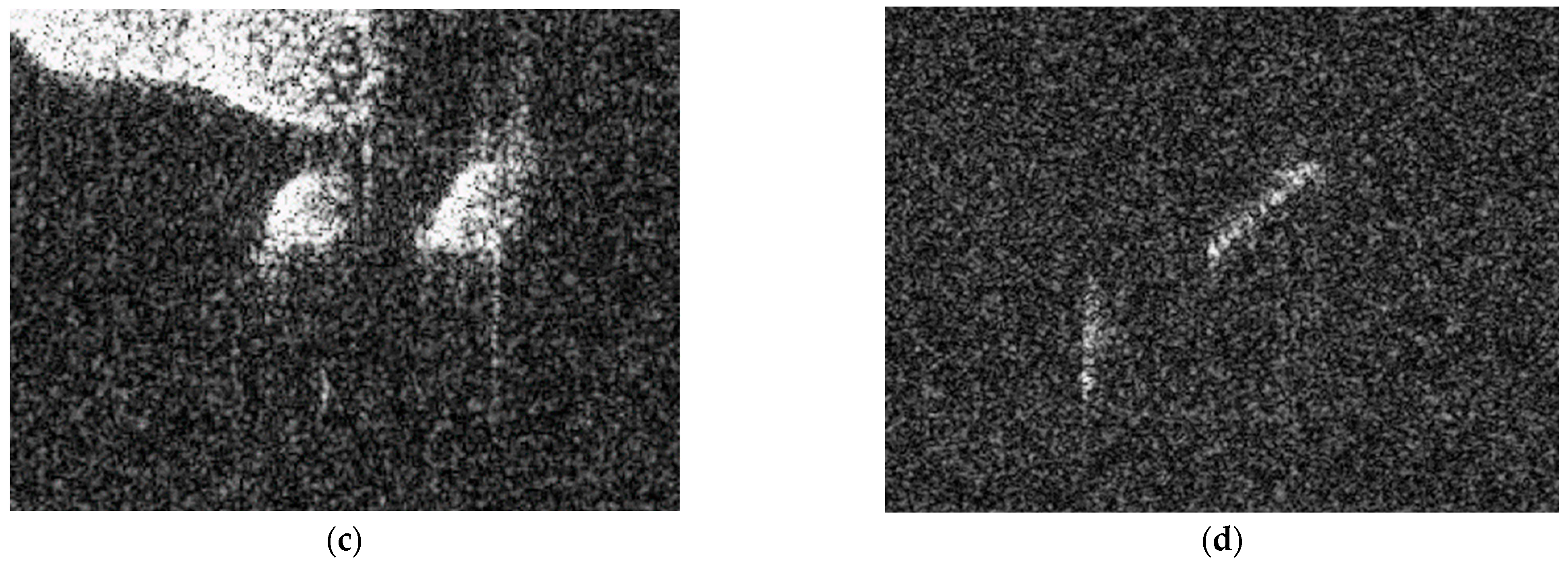
One labeled image is shown in Figure 5a, and Figure 5b–d gives the three local close-ups. Figure 5b shows a patch containing a labeled ship. Figure 5c,d illustrates two patches containing an island and an azimuth ambiguity respectively, which are similar with ships and thus are prone to form false alarms, indicating the challenge of the task.

3.2. Experimental Setup and Evaluation Index

We implement the proposed algorithm through python 3.6 and the open-source deep learning library PyTorch 1.9.0, and execute it on a 64-bit Ubuntu 20.04 workstation with 12 GB memory GeForce RTX3060 GPU. In the improved CSSL pre-training stage, the SGD method is used to train 20 epochs for the proposed network. The batch size is set as 32, the initial learning rate is set as 0.002, and the momentum and weight decay are set as 0.9 and 0.0005, respectively. The argument $\alpha$ for the mixed coefficient resulting from the beta distribution is set as 1.0, $\mu$ in the final loss is set as 0.5. In the Faster R-CNN network training stage, the SGD method is used to train 20 epochs for the Faster R-CNN network. The batch size is set as 8, the initial learning rate is set as 0.005, and the momentum and weight decay are set as 0.9 and 0.0005, respectively. In the first five epochs of training, we freeze the feature extraction network weights, then train the RPN network and the detection network. In the subsequent 15 epochs of training, we un-freeze the feature extraction network weights, and train all network parameters at the same time.

The evaluation indicator is the standard to measure the training effect of the model. In the process of our model’s training and testing, accuracy, precision, recall, and mean average precision (mAP) are mainly selected as the evaluation indicators. The combination of sample real class and model prediction class is divided into four cases: true positive, false positive, true negative and false negative. We denote them by $TP$, $FP$, $TN$ and $FN$ respectively. Obviously, $TP$ + $FP$ + $TN$ + $FN$ = total number of samples.

$Accuracy$ means the ratio of correct prediction made by the model, which is defined as:

$$Accuracy=\frac{TP+TN}{TP+FP+TN+FN}.$$

(30)

$Precision$ means the ratio of actually positive examples in the examples divided into positive examples. In the case of un-balanced positive and negative samples, the $Accuracy$ will have problems in measuring the prediction effect of the model, and the $Precision$ makes up for this defect. $Precision$ is defined as:

$$Precision=\frac{TP}{TP+FP}.$$

(31)

$Recall$ means the ratio of positive samples predicted as positive samples in the total positive samples, reflecting the comprehensiveness of the model’s prediction of positive samples, which is defined as:

$$Recall=\frac{TP}{TP+FN}.$$

(32)

Mean Average Precision (mAP) means the mean value of all classifications’ AP. Since there is only one classification (ship), mAP = AP. AP defined as the area under the precision-recall curve.

3.3. PolSAR Ship Detection Experiments

3.3.1. Ablation Experiments

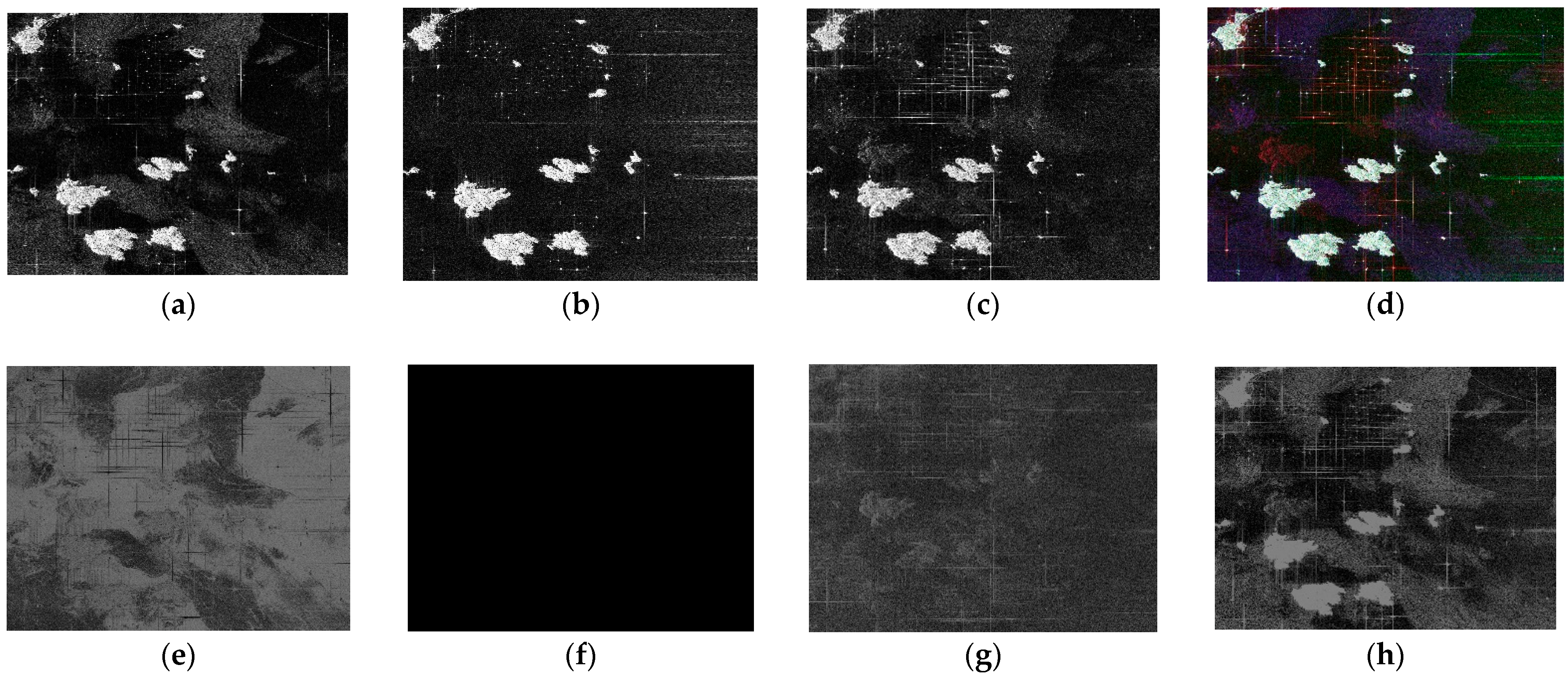
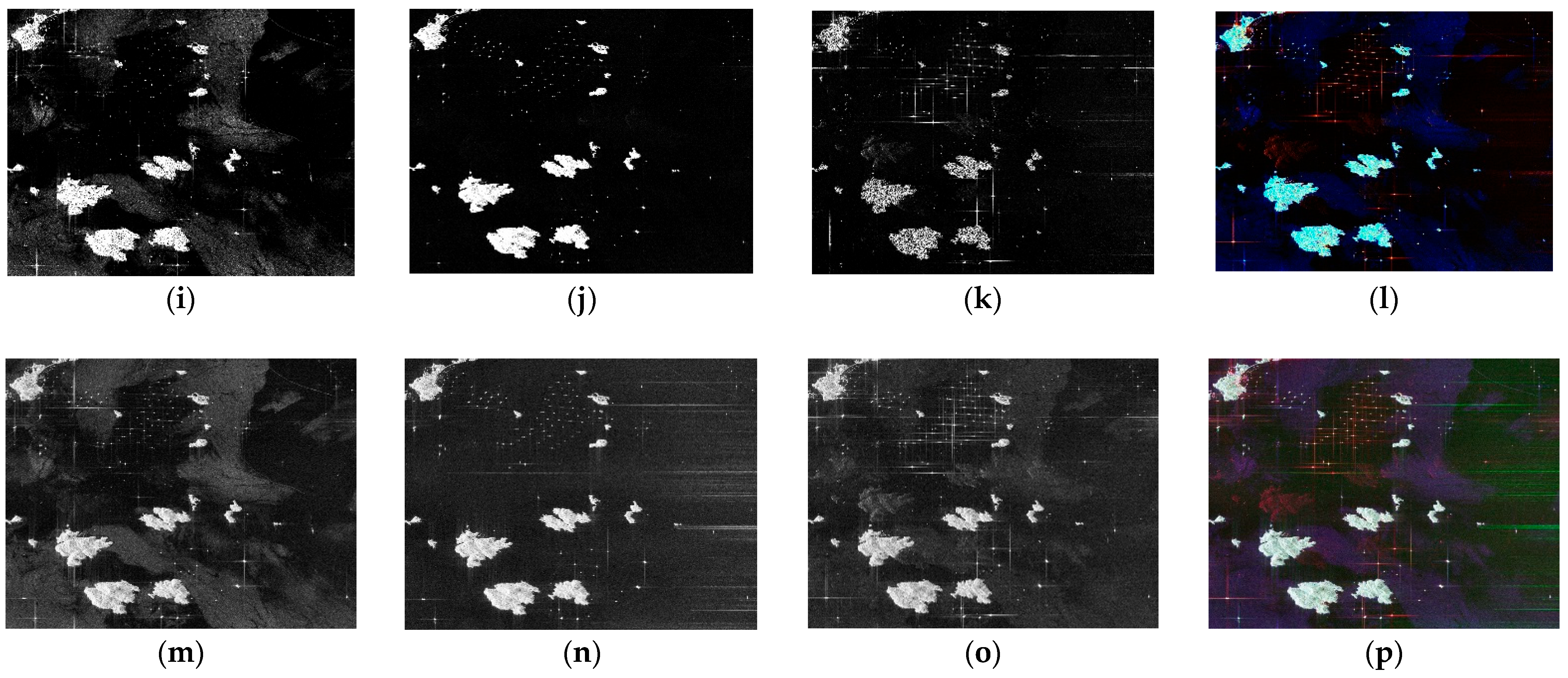
In the experiments, we extracted the polarimetric features of the original PolSAR images and constructed multi-channel input data through Pauli, Cloude, Freeman, Yamaguchi, Cui, Coherence, Refined Lee and Adaptive methods. The constructed input image is shown in Figure 6. The number of channels of the input image obtained by different polarimetric feature extraction methods is different, methods Cloude and Yamaguchi obtaine 4-channel images, and other methods obtaine 3-channel images. As shown in Figure 6a–c, the three images obtained by Pauli decomposition respectively represent: odd-bounce scattering energy, corresponding to channel B; volume scattering energy, corresponding to channel G; and double-bounce scattering energy, corresponding to channel R. Figure 6d is the pseudo-color image of above, that is, the multi-channel input data. Similarly, Figure 6e–h show the polarization entropy, average of scattering angles, polarization anti-entropy, and scattering power SPAN obtained by Cloude decomposition. Figure 6i–k show the surface, volume, and double-bounce scattering obtained by Cui decomposition. Figure 6m–o show the images obtained by Pauli decomposition after Adaptive filtering. The images obtained by Freeman and Yamaguchi are similar in appearance to those obtained by Cui, the images obtained by Refined Lee are similar in appearance to those obtained by Adaptive, and the images obtained by Coherence are very dark because of the value is within [0,1). Therefore, the images of the remaining four methods will not be shown. Input data containing multiple polarimetric features are used in subsequent experiments to study the effect of various factors on the detection results.

Firstly, we explored the effect of the input data constructed by eight polarimetric feature extraction methods on the detection results. Quantitative results comparison is summarized in

Table 1. Ship detection results (AP) with different input factors.

	Train with Our Method				Train from Scratch
	All Data	100-Shot	50-Shot	30-Shot	All Data	100-Shot	50-Shot	30-Shot
Pauli	0.93	0.859	0.594	0.127	0.887	0.801	0.505	0.013
Cloude	0.756	0.594	0.192	0.034	0.634	0.423	0.078	0.01
Freeman	0.83	0.772	0.468	0.035	0.781	0.586	0.382	0.006
Yamaguchi	0.861	0.667	0.296	0.089	0.785	0.631	0.073	0.01
Cui	0.921	0.792	0.673	0.333	0.836	0.679	0.514	0.167
Coherence	0.325	0.142	0.03	0.029	0.093	0.057	0.005	0
Refined Lee	0.931	0.897	0.696	0.267	0.898	0.842	0.634	0.118
Adaptive	0.935	0.877	0.655	0.483	0.901	0.816	0.556	0.11

. As seen from the detection results, after the pre-training of our method under the input of all data which contains 198 labeled samples, the Adaptive method achieves the best detection result of 0.935 (AP). The detection results of the Refined Lee method, which is also a speckle filtering method as same as the Adaptive method, and the Pauli method, which is the basis of the two speckle filtering methods, both exceeding 0.93 together. The Cui method is one of the three polarization decomposition methods based on scattering model, and its detection result exceeding 0.9, reaching 0.921. The above four methods also obtain better detection results than other methods in the case of other input sample numbers and train from scratch [55]. In addition, the detection result of the Coherence method is the worst, which is less than 0.325. The huge difference of the detection results obtained by different polarimetric feature inputs proves that selecting the appropriate polarimetric feature extraction method is helpful to improve the effect of ship detection.

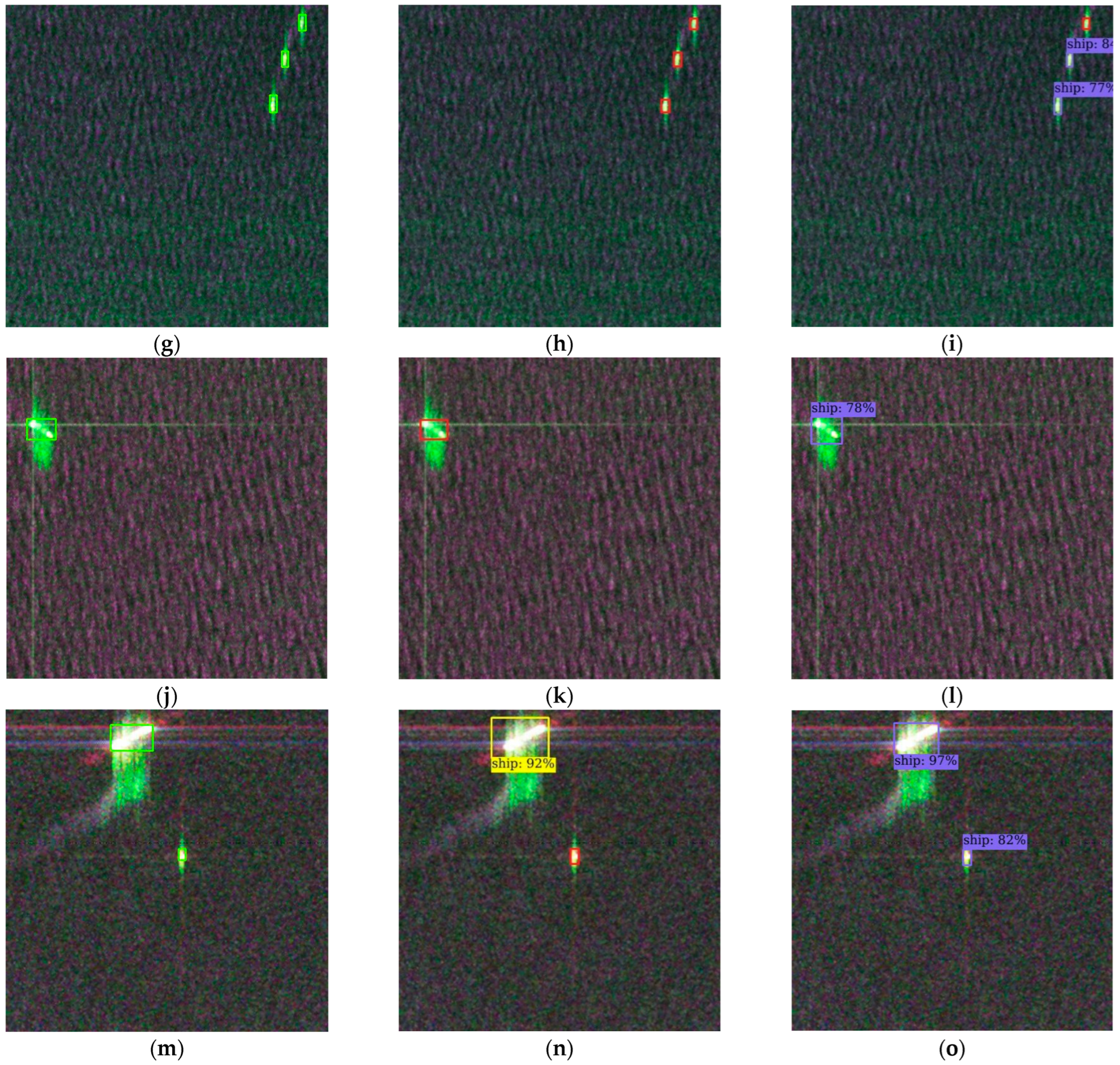
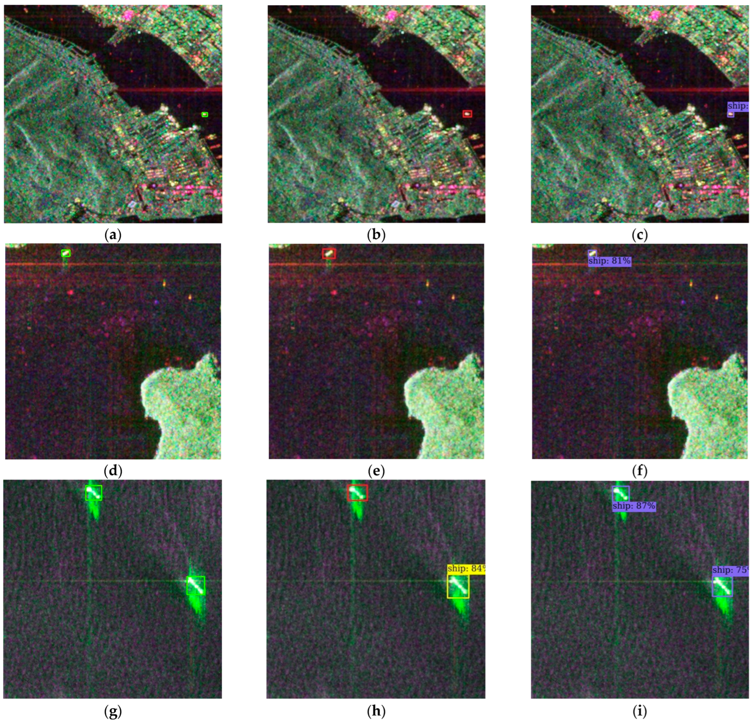
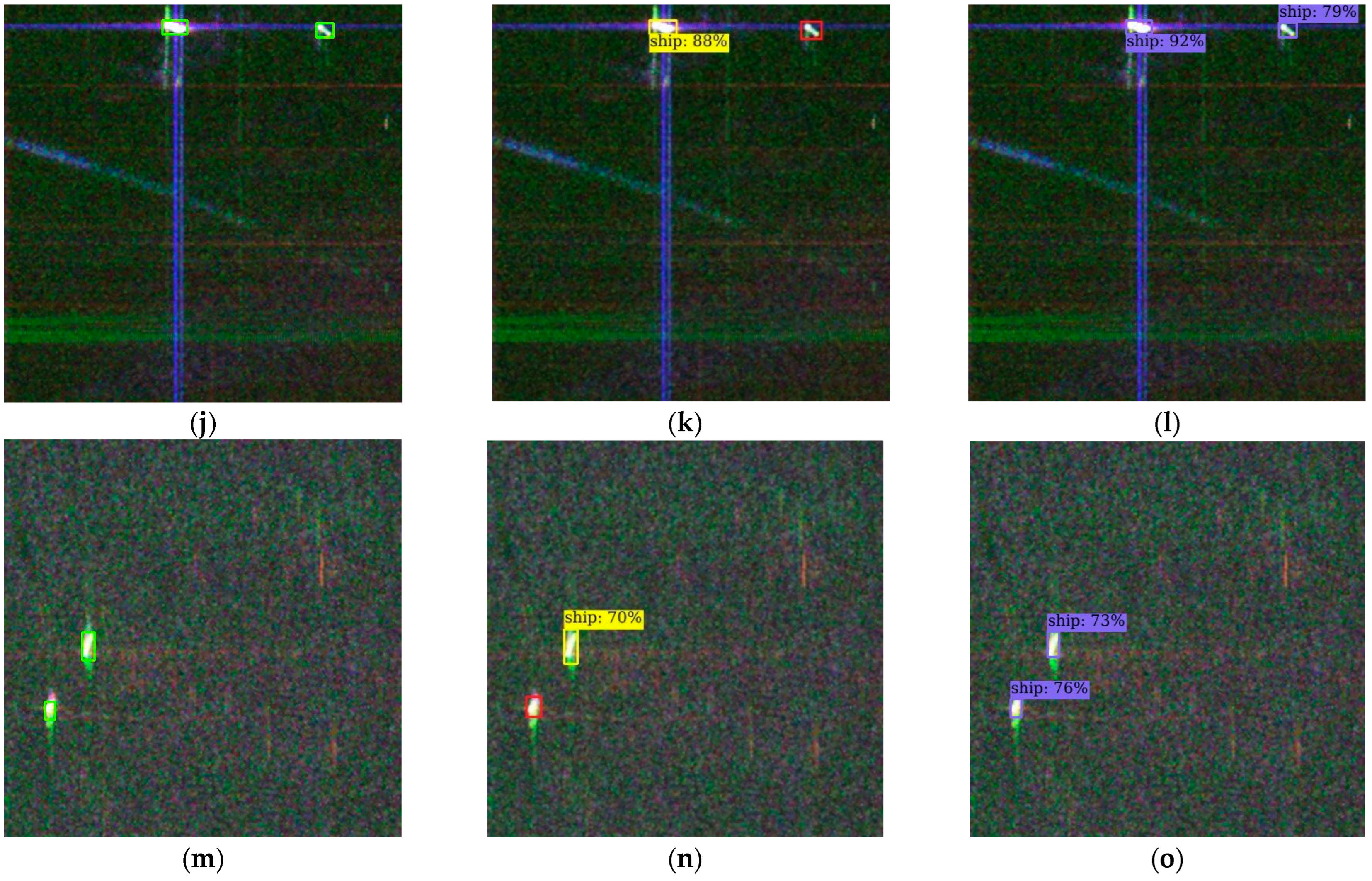
Secondly, we compared the ship detection results with and without pre-training under different training sample numbers. As shown in Table 1, under the factors of 8 polarimetric feature inputs and four kinds of input sample numbers, the detection results have been improved after the pre-training of the proposed method. The visualization of detection results is shown in Figure 7. Specifically, Figure 7a–c show that after pre-training, the false detection caused by near-shore has been avoided, and one of the two near-shore ships has been successfully detected; Figure 7d–f show that the missed detection caused by sidelobe is successfully detected after pre-training; Figure 7g–i show that after pre training, two of the three missed detections caused by dense targets have been successfully detected; Figure 7j–l show that, the missed detection caused by defocusing is successfully detected after pre training; Figure 7m–o show that the missed detection caused by small targets is successfully detected after pre-training. As seen from Figure 8, under some polarimetric feature input factors, when the number of input samples decreases, the detection result will decrease rapidly. For example, when the number of input samples of Cloude method decreases from 100-shot to 50-shot, and when the number of input samples of Pauli, Freeman, and Refined Lee method decreases from 50-shot to 30-shot, the detection results decreases by more than 0.4 (AP). This shows that although pre-training can improve the detection effect on few-shot PolSAR ship detection task, when the number of input samples is reduced to a certain threshold, the generalization ability of the model will be insufficient.

Finally, we compared the original contrastive learning method with the proposed improved CSSL method and presented ablation experiments on each module of the proposed method to understand their effectiveness. The results are shown in

Table 2. Ship detection results (AP) of different pre-training methods.

Method	Average Precision (AP)
Original SimSiam	0.919
SimSiam and MFFM	0.923
SimSiam and MUAP	0.929
Our method	0.935

. The polarimetric feature extraction method of the input data adopts the Adaptive method. After the original SimSiam method is optimized by the MFFM module and the MUAP module, respectively, the ship detection results are improved, which shows that both modules contribute to improving the performance of the pre-training network. We also conducted experiments on the effect of different structures of backbone on the detection results, including ResNet-18, ResNet-34, ResNet-50 and ResNet-101. The polarimetric feature extraction method of the input data is the Adaptive method, and the results are shown in

Table 3. Ship detection results (AP) of different structures of backbone.

	Train with Our Method	Train from Scratch
ResNet-18	0.935	0.901
ResNet-34	0.942	0.923
ResNet-50	0.902	0.854
ResNet-101	0.87	0.739

. When the backbone is ResNet-34, the best detection result is obtained, which is 0.942, followed by ResNet-18, which is reduced by 0.007. Considering the efficiency of pre-training, we chose ResNet-18 as the backbone of our method.

3.3.2. Comparison Experiments

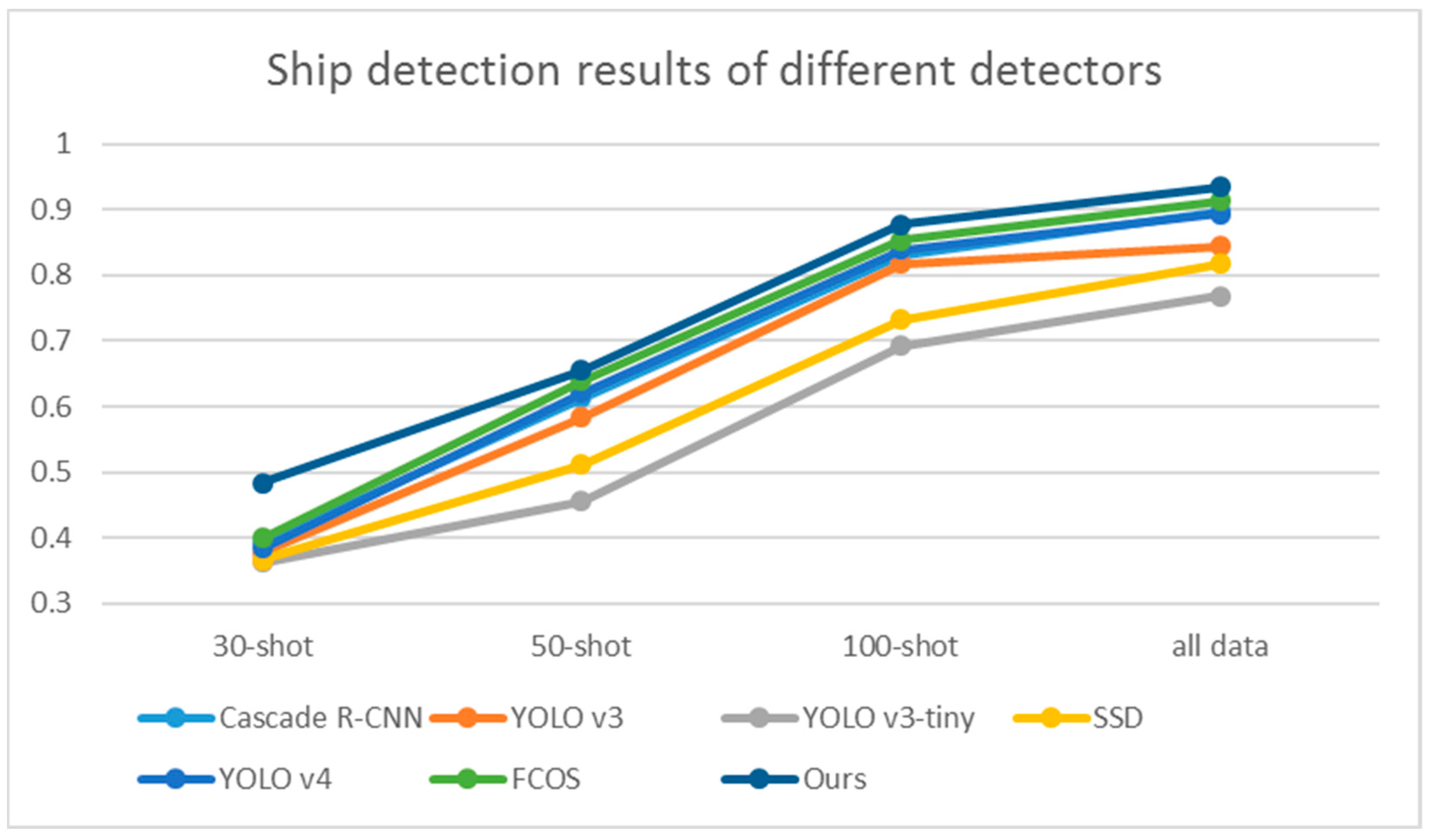
We compared our method with some classic target detectors, including Cascade R-CNN [56], YOLO v3 [57], YOLO v3-tiny [58], SSD [59], YOLO v4 [60] and FCOS [61]. The polarimetric feature extraction method of the input data adopts the Adaptive method, and the backbone adopts ResNet-18. The results are shown in

Table 4. Ship detection results (AP) of different detectors.

	All Data	100-Shot	50-Shot	30-Shot
Cascade R-CNN	0.898	0.831	0.612	0.392
YOLO v3	0.844	0.817	0.583	0.377
YOLO v3-tiny	0.769	0.693	0.456	0.362
SSD	0.818	0.733	0.511	0.366
YOLO v4	0.894	0.839	0.62	0.384
FCOS	0.914	0.853	0.639	0.4
Ours	0.935	0.877	0.655	0.483

. It can be observed that our method has achieved the best detection results under the factors of each input sample number. The test result next to our method is the FCOS method, and the worst detection result is YOLO v3-tiny method. The visualization of detection results is shown in Figure 9. Specifically, Figure 9a–c show that the missed detection caused by complex background and small targets that cannot be detected by all classic detectors has been successfully detected by our method; Figure 9d–f show that the missed detection caused by proximity to edges and small targets that cannot be detected by all classic detectors except SSD has been successfully detected by our method; Figure 9g–i show that the missed detection caused by defocusing that cannot be detected by only SSD method has been successfully detected by our method; Figure 9j–l show that the missed detection caused by proximity to edges and small targets that cannot be detected by YOLO v3, YOLO v3-tiny, and FCOS methods has been successfully detected by our method; Figure 9m–o show that the missed detection caused by small targets that cannot be detected by Cascade R-CNN, SSD, YOLO v3, and YOLO v4 methods has been successfully detected by our method. By comparing the test results with the FCOS method under the factors of different input sample numbers, it can be seen from Figure 10 that our method has made a great improvement in the case of a few numbers of training samples. The comparison with other detectors also confirmed this point. In conclusion, the results of comparison experiments verify the effectiveness of our method in few-shot PolSAR ship detection task.

Our method applies the pre-trained backbone to the downstream target detection network. Only a few labeled samples are used for fine-tuning to achieve the few-shot PolSAR ship detection effect. Therefore, our method does not depend on the target detection framework. To better demonstrate the effectiveness of our proposed methodology and its adaptability to different ship detection frameworks, we replaced the Faster-RCNN baseline with YOLO v5 [62] and FCOS. Specifically, the original backbone networks of YOLO v5 and FCOS will be replaced by our pre-trained ResNet-18 with the FMMF module, while other components, such as the neck module, will be retained. The results are presented in

Table 5. Ship detection results (AP) of different target detection frameworks.

Method	All Data	100-Shot	50-Shot	30-Shot
Faster R-CNN	0.901	0.816	0.556	0.11
Faster R-CNN and pre-training	0.935	0.877	0.655	0.483
YOLO v5	0.887	0.838	0.612	0.389
YOLO v5 and pre-training	0.939	0.894	0.696	0.552
FCOS	0.914	0.853	0.639	0.4
FCOS and pre-training	0.942	0.903	0.717	0.583

. From the table, it is evident that the YOLO v5 and FCOS networks, enhanced through our pre-training methodology, exhibit improved performance compared to their original versions. Therefore, it can be concluded that the effectiveness of our proposed methodology is universally applicable and does not depend on a specific object detection framework.

In order to demonstrate the superiority of our proposed method, we make a comparison with two state-of-the-art few-shot learning methods, including SAMBFS-FSDet [63] and G-FSDet [64]. As for the two methods, Faster R-CNN and TFA [65] are used for the few-shot object detection framework. In the fine-tuning stage, we use the previously labeled ship samples as the novel classes to achieve a few-shot ship detection target. The comparison results are presented in

Table 6. Ship detection results (AP) of different few-shot learning methods.

	All Data	100-Shot	50-Shot	30-Shot
SAMBFS-FSDet	0.893	0.805	0.551	0.433
G-FSDet	0.904	0.824	0.577	0.456
Ours	0.935	0.877	0.655	0.483

. From the table, it can be observed that our proposed method is still competitive compared to the state-of-the-art few-shot learning methods.

4. Discussion

By analyzing the effect of eight polarimetric feature extraction methods in Table 1 on the detection results, we find that the input data constructed by Pauli decomposition, Refined Lee filtering and Adaptive filtering have achieved good detection results, exceeding 0.93 (AP). Since the Refined Lee filtering and Adaptive filtering are speckle filtering methods based on the Pauli decomposition, this shows that the Pauli decomposition method extracts more effective polarimetric and spatial features. Through speckle filtering, the spatial features are further enhanced at the cost of a certain loss of the polarimetric features. The detection results of the two speckle filtering methods are better than those of the original Pauli decomposition method, indicating that our method is more sensitive to the spatial features of the target. Freeman, Yamaguchi and Cui are polarization decomposition methods based on scattering models. Yamaguchi adds a helix component on the basis of Freeman. Cui exactly accounts for every element of the observed coherency matrix compared with Freeman and Yamaguchi. According to the detection results in Table 1, the detection effect of these three methods will increase with the increase in the fineness of the model. This means that extracting better polarimetric features as input will help increase the detection effect of our model. The detection effects of Cloude decomposition and polarimetric coherence are poor, which may be due to the insufficient power features extracted by these methods. Cloude decomposition presents power features as a single channel image SPAN, while polarimetric coherence does not contain power features.

Through the comparison of the effect of whether to use CSSL pre-training and different numbers of input samples on the test results, it can be seen from Table 1 that after pre-training, the detection ability of the model has improved under each case of input samples, with an average improvement of 0.084 in the case of all-data, 0.096 in the case of 100-shot, 0.107 in the case of 50-shot, and 0.12 in the case of 30-shot. It shows that the smaller the number of input samples, the more obvious the improvement in the detection ability. Figure 8 also shows the situation intuitively.

To further study the effect of the depth of ResNet as the backbone network on ship detection results, several typical ResNets are selected for ablation experiments. As shown in Table 3, ResNet-34 was used as the feature extraction backbone and achieved the best ship detection results. With the increase in network layers, the detection effect shows a trend of improving first and then decreasing. This indicates that the network can learn features better when the number of network layers increases, but when the number of network layers is too large, the network cannot be well fitted due to a lack of training samples. Finally, we chose ResNet-18 as the backbone network. The ResNet-18 network is chosen as the feature extraction backbone because of its high training efficiency and ability to maintain good detection results.

Compared with several ship detection methods, our proposed method has improved the feature extraction ability of the network, especially under the few-shot conditions, but further work is still needed to improve the detection performance. In addition, when the number of input samples is too small, the test results will drop significantly. This shows that although pre-training can improve the detection effect on a few-shot PolSAR ship detection task, when the number of input samples is reduced to a certain threshold, the generalization ability of the model will be insufficient. Other factors, such as the number of backbone layers, the input data selection with polarimetric features, and the ship detection framework, also have a certain impact. This is the limitation of our method. The core idea of this work is to find the best combination of input data with polarimetric features and increase detection performance by optimizing the backbone network.

5. Conclusions

In this paper, an improved CSSL-based PolSAR ship detection method is proposed. Based on the contrastive learning framework without negative samples, MFFM and MUAP modules were used to optimize it, and the un-labeled PolSAR data were fully exploited for pre-training to achieve efficient feature extraction capability. In addition, the effect of the input data construction with different polarimetric features, the backbone network selection, and the number of input samples on the detection results was also explored. The ablation and comparison experiments were conducted on the GF-3 dataset. The ablation experiments investigated the effect of each module of the proposed method on detection performance, which validated their effectiveness. The results of the comparison experiments demonstrated the superiority of the proposed method compared with other deep learning methods in few-shot PolSAR ship detection tasks. We will focus on how to better solve the few-shot PolSAR ship detection task in our future work.

References

1. Moreira, A.; Iraola, P.; Younis, M.; Krieger, G.; Hajnsek, I.; Papathanassiou, K.P. A Tutorial on Synthetic Aperture Radar. IEEE Geosci. Remote Sens. Mag. 2013, 1, 6–43. [Google Scholar] [CrossRef] [Green Version]
2. Touzi, R.; Boerner, W.M.; Lee, J.S.; Lueneburg, E. A Review of Polarimetry in the Context of Synthetic Aperture Radar: Concepts and Information Extraction. Can. J. Remote Sens. 2004, 30, 380–407. [Google Scholar] [CrossRef]
3. Leng, X.; Ji, K.; Yang, K.; Zou, H. A Bilateral CFAR Algorithm for Ship Detection in SAR Images. IEEE Geosci. Remote Sens. Lett. 2015, 7, 1536–1540. [Google Scholar] [CrossRef]
4. Gao, G.; Luo, Y.; Ouyang, K.; Zhou, S. Statistical Modeling of PMA Detector for Ship Detection in High-Resolution Dual-Polarization SAR Images. IEEE Trans. Geosci. Remote Sens. 2016, 54, 4302–4313. [Google Scholar] [CrossRef]
5. Gao, G.; Ouyang, K.; Luo, Y.; Liang, S.; Zhou, S. Scheme of Parameter Estimation for Generalized Gamma Distribution and Its Application to Ship Detection in SAR Images. IEEE Trans. Geosci. Remote Sens. 2017, 55, 1812–1832. [Google Scholar] [CrossRef]
6. Gao, G.; Li, G.; Li, Y. Shape Parameter Estimator of the Generalized Gaussian Distribution Based on the MoLC. IEEE Geosci. Remote Sens. Lett. 2018, 15, 350–354. [Google Scholar] [CrossRef]
7. Tao, D.; Anfinsen, S.N.; Brekke, C. Robust CFAR Detector Based on Truncated Statistics in Multiple-Target Situations. IEEE Trans. Geosci. Remote Sens. 2016, 54, 117–134. [Google Scholar] [CrossRef]
8. Liu, T.; Yang, Z.; Marino, A.; Gao, G.; Yang, J. Robust CFAR Detector Based on Truncated Statistics for Polarimetric Synthetic Aperture Radar. IEEE Trans. Geosci. Remote Sens. 2020, 58, 6731–6747. [Google Scholar] [CrossRef]
9. Ringrose, R.; Harris, N. Ship Detection Using Polarimetric SAR Data. In Proceedings of the CEOS SAR Workshop, Toulouse, France, 26–29 October 1999. [Google Scholar]
10. Touzi, R.; Charbonneau, F.; Hawkins, R.K.; Murnaghan, K.; Kavoun, X. Ship-Sea Contrast Optimization When Using Polarimetric SARs. In Proceedings of the IEEE 2001 International Geoscience and Remote Sensing Symposium (IGARSS), Sydney, Australia, 9–13 July 2001. [Google Scholar]
11. Chen, J.; Chen, Y.; Yang, J. Ship Detection Using Polarization Cross-Entropy. IEEE Geosci. Remote Sens. Lett. 2009, 6, 723–727. [Google Scholar] [CrossRef]
12. Sugimoto, M.; Ouchi, K.; Nakamura, Y. On the Novel Use of Model-Based Decomposition in SAR Polarimetry for Target Detection on the Sea. Remote Sens. Lett. 2013, 4, 843–852. [Google Scholar] [CrossRef]
13. Yang, J.; Dong, G.; Peng, Y.; Yamaguchi, Y.; Yamada, H. Generalized Optimization of Polarimetric Contrast Enhancement. IEEE Geosci. Remote Sens. Lett. 2004, 1, 171–174. [Google Scholar] [CrossRef]
14. Yin, J.; Yang, J.; Xie, C.; Zhang, Q.; Li, Y.; Qi, Y. An Improved Generalized Optimization of Polarimetric Contrast Enhancement and Its Application to Ship Detection. IEICE Trans. Commun. 2013, 96, 2005–2013. [Google Scholar] [CrossRef]
15. Gao, G.; Gao, S.; He, J.; Li, G. Ship Detection Using Compact Polarimetric SAR Based on the Notch Filter. IEEE Trans. Geosci. Remote Sens. 2018, 56, 5380–5393. [Google Scholar] [CrossRef]
16. Xu, Z.; Tang, B.; Cheng, S. Faint Ship Wake Detection in PolSAR Images. IEEE Geosci. Remote Sens. Lett. 2018, 15, 1055–1059. [Google Scholar] [CrossRef]
17. Kaplan, L.M. Improved SAR Target Detection via Extended Fractal Features. IEEE Trans. Aeros. Electron. Syst. 2001, 37, 436–451. [Google Scholar] [CrossRef]
18. De Grandi, G.D.; Lee, J.; Schuler, D.L. Target Detection and Texture Segmentation in Polarimetric SAR Images Using a Wavelet Frame: Theoretical Aspects. IEEE Trans. Geosci. Remote Sens. 2007, 45, 3437–3453. [Google Scholar] [CrossRef]
19. Li, J.; Qu, C.; Shao, J. Ship Detection in SAR Images Based on an Improved Faster R-CNN. In Proceedings of the 2017 SAR in Big Data Era: Models, Methods and Applications, Beijing, China, 13–14 November 2017. [Google Scholar]
20. Lin, Z.; Ji, K.; Leng, X.; Kuang, G. Squeeze and Excitation Rank Faster R-CNN for Ship Detection in SAR Images. IEEE Geosci. Remote Sens. Lett. 2019, 16, 751–755. [Google Scholar] [CrossRef]
21. Wang, Z.; Du, L.; Mao, J.; Liu, B.; Yang, D. SAR Target Detection Based on SSD with Data Augmentation and Transfer Learning. IEEE Geosci. Remote Sens. Lett. 2019, 16, 150–154. [Google Scholar] [CrossRef]
22. Zhang, T.; Zhang, X.; Shi, J.; Wei, W. High-Speed Ship Detection in SAR Images by Improved Yolov3. In Proceedings of the 2019 16th International Computer Conference on Wavelet Active Media Technology and Information Processing, Chengdu, China, 14–15 December 2019. [Google Scholar]
23. Zhu, M.; Hu, G.; Zhou, H.; Wang, S.; Feng, Z.; Yue, S. A Ship Detection Method via Redesigned FCOS in Large-Scale SAR Images. Remote Sens. 2022, 14, 1153. [Google Scholar] [CrossRef]
24. Zhu, M.; Hu, G.; Li, S.; Zhou, H.; Wang, S.; Feng, Z. A Novel Anchor-Free Method Based on FCOS + ATSS for Ship Detection in SAR Images. Remote Sens. 2022, 14, 2034. [Google Scholar] [CrossRef]
25. Chen, S.; Li, Y.; Wang, X.; Xiao, S.; Sato, M. Modeling and Interpretation of Scattering Mechanisms in Polarimetric Synthetic Aperture Radar: Advances and perspectives. IEEE Signal Proc. Mag. 2014, 31, 79–89. [Google Scholar] [CrossRef]
26. Chen, S.; Wang, X.; Xiao, S.; Sato, M. Target Scattering Mechanism in Polarimetric Synthetic Aperture Radar: Interpretation and Application; Springer: Singapore, 2018; pp. 1–225. [Google Scholar]
27. Rostami, M.; Kolouri, S.; Eaton, E.; Kim, K. Deep Transfer Learning for Few-Shot SAR Image Classification. Remote Sens. 2019, 11, 1374. [Google Scholar] [CrossRef] [Green Version]
28. Rostami, M.; Kolouri, S.; Eaton, E.; Kim, K. SAR Image Classification Using Few-Shot Cross-Domain Transfer Learning. In Proceedings of the 2019 IEEE Conference on Computer Vision and Pattern Recognition (CVPR), Longbeach, CA, USA, 16–20 June 2019. [Google Scholar]
29. Wang, L.; Bai, X.; Gong, C.; Zhou, F. Hybrid Inference Network for Few-Shot SAR Automatic Target Recognition. IEEE Trans. Geosci. Remote Sens. 2021, 59, 9257–9269. [Google Scholar] [CrossRef]
30. Fu, K.; Zhang, T.; Zhang, Y.; Wang, Z.; Sun, X. Few-Shot SAR Target Classification via Metalearning. IEEE Trans. Geosci. Remote Sens. 2021, 60, 1–14. [Google Scholar] [CrossRef]
31. Huang, Z.; Pan, Z.; Lei, B. What, Where, and How to Transfer in SAR Target Recognition Based on Deep CNNs. IEEE Trans. Geosci. Remote Sens. 2019, 58, 2324–2336. [Google Scholar] [CrossRef] [Green Version]
32. He, K.; Fan, H.; Wu, Y.; Xie, S.; Girshick, R. Momentum Contrast for Unsupervised Visual Representation Learning. In Proceedings of the IEEE/CVF Conference on Computer Vision and Pattern Recognition (CVPR), Seattle, WA, USA, 13–19 June 2020. [Google Scholar]
33. Chen, T.; Kornblith, S.; Norouzi, M.; Hinton, G. A Simple Framework for Contrastive Learning of Visual Representations. In Proceedings of the IEEE Conference on Computer Vision and Pattern Recognition (CVPR), Seattle, WA, USA, 13–19 June 2020. [Google Scholar]
34. Grill, J.B.; Strub, F.; Altché, F.; Tallec, C.; Richemond, P.; Buchatskaya, E.; Doersch, C.; Pires, B.A.; Guo, Z.; Azar, M.G.; et al. Bootstrap Your Own Latent-A New Approach to Self-Supervised Learning. Adv. Neural Inf. Process. Syst. 2020, 33, 21271–21284. [Google Scholar]
35. Chen, X.; He, K. Exploring Simple Siamese Representation Learning. In Proceedings of the IEEE/CVF Conference on Computer Vision and Pattern Recognition (CVPR), Nashville, TN, USA, 20–25 June 2021. [Google Scholar]
36. Wang, D.; Zhang, J.; Du, B.; Xia, G.S.; Tao, D. An Empirical Study of Remote Sensing Pretraining. arXiv 2022, arXiv:2204.02825. [Google Scholar] [CrossRef]
37. Zhang, L.; Zhang, S.; Zou, B.; Dong, H. Unsupervised Deep Representation Learning and Few-Shot Classification of PolSAR Images. IEEE Trans. Geosci. Remote Sens. 2020, 60, 1–16. [Google Scholar] [CrossRef]
38. Yang, M.; Jiao, L.; Liu, F.; Hou, B.; Yang, S.; Zhang, Y.; Wang, J. Coarse-to-Fine Contrastive Self-Supervised Feature Learning for Land-Cover Classification in SAR Images with Limited Labeled Data. IEEE Trans. Image Process. 2022, 31, 6502–6516. [Google Scholar] [CrossRef]
39. He, K.; Zhang, X.; Ren, S.; Sun, J. Deep Residual Learning for Image Recognition. In Proceedings of the IEEE Conference on Computer Vision and Pattern Recognition (CVPR), Las Vegas, NV, USA, 27–30 June 2016. [Google Scholar]
40. Ren, S.; He, K.; Girshick, R.; Sun, J. Faster R-CNN: Towards Real-Time Object Detection with Region Proposal Networks. IEEE Trans. Pattern Anal. Mach. Intell. 2017, 39, 1137–1149. [Google Scholar] [CrossRef] [Green Version]
41. Cloude, S.R. Target Decomposition Theorems in Radar Scattering. Electron. Lett. 2007, 21, 22–24. [Google Scholar] [CrossRef]
42. Cloude, S.R.; Pottier, E. An Entropy Based Classification Scheme for Land Applications of Polarimetric SAR. IEEE Trans. Geosci. Remote Sens. 1997, 35, 68–78. [Google Scholar] [CrossRef]
43. Freeman, A.; Durden, S.L. A Three-Component Scattering Model for Polarimetric SAR Data. IEEE Trans. Geosci. Remote Sens. 1998, 36, 963–973. [Google Scholar] [CrossRef] [Green Version]
44. Yamaguchi, Y.; Moriyama, T.; Ishido, M.; Yamada, H. Four Component Scattering Model for Polarimetric SAR Image Decomposition. IEEE Trans. Geosci. Remote Sens. 2005, 43, 1699–1706. [Google Scholar] [CrossRef]
45. Cui, Y.; Yamaguchi, Y.; Yang, J.; Kobayashi, H.; Park, S.; Singh, G. On Complete Model-Based Decomposition of Polarimetric SAR Coherency Matrix Data. IEEE Trans. Geosci. Remote Sens. 2014, 52, 1991–2001. [Google Scholar] [CrossRef]
46. Touzi, R.; Lopes, A.; Bruniquel, J.; Vachon, P.W. Coherence Estimation for SAR Imagery. IEEE Trans. Geosci. Remote Sens. 1999, 37, 135–149. [Google Scholar] [CrossRef] [Green Version]
47. Lee, J.; Grunes, M.R.; Grandi, G. Polarimetric SAR Speckle Filtering and Its Implication for Cassification. IEEE Trans. Geosci. Remote Sens. 1999, 37, 2363–2373. [Google Scholar]
48. Lang, F.; Yang, J.; Li, D. Adaptive-Window Polarimetric SAR Image Speckle Filtering Based on a Homogeneity Measurement. IEEE Trans. Geosci. Remote Sens. 2015, 53, 5435–5446. [Google Scholar] [CrossRef]
49. Cloude, S.R.; Pottier, E. A Review of Target Decomposition Theorems in Radar Polarimetry. IEEE Trans. Geosci. Remote Sens. 1996, 34, 498–518. [Google Scholar] [CrossRef]
50. Goodman, J.W. Some Fundamental Properties of Speckle. J. Opt. Soc. Am. 1976, 66, 1145–1150. [Google Scholar] [CrossRef]
51. Chen, L.C.; Papandreou, G.; Kokkinos, I.; Murphy, K.; Yuille, A.L. DeepLab: Semantic Image Segmentation with Deep Convolutional Nets, Atrous Convolution, and Fully Connected CRFs. IEEE Trans. Pattern Anal. Mach. Intell. 2018, 40, 834–848. [Google Scholar] [CrossRef] [PubMed] [Green Version]
52. Zhang, H.; Cisse, M.; Dauphin, Y.N.; Lopez-Paz, D. Mixup: Beyond Empirical Risk Minimization. arXiv 2018, arXiv:1710.09412. [Google Scholar]
53. Guo, X.; Zhao, T.; Lin, Y.; Du, B. MixSiam: A Mixture-Based Approach to Self-Supervised Representation Learning. arXiv 2021, arXiv:2111.02679. [Google Scholar]
54. Pang, D.; Pan, C.; Zi, X. GF-3: The Watcher of the Vast Territory. Aerosp. China 2016, 9, 8–12. [Google Scholar]
55. Shen, Z.; Liu, Z.; Li, J.; Jiang, Y.; Chen, Y.; Xue, X. DSOD: Learning Deeply Supervised Object Detectors from Scratch. In Proceedings of the IEEE International Conference on Computer Vision (ICCV), Venice, Italy, 22–29 October 2017. [Google Scholar]
56. Cai, Z.; Vasconcelos, N. Cascade R-CNN: Delving into High Quality Object Detection. In Proceedings of the IEEE Conference on Computer Vision and Pattern Recognition (CVPR), Salt Lake City, UT, USA, 18–22 June 2018. [Google Scholar]
57. Redmon, J.; Farhadi, A. YOLOv3: An Incremental Improvement. arXiv 2018, arXiv:1804.02767. [Google Scholar]
58. Adarsh, P.; Rathi, P.; Kumar, M. YOLO v3-Tiny: Object Detection and Recognition Using One Stage Improved Model. In Proceedings of the 2020 6th International Conference on Advanced Computing and Communication Systems (ICACCS), Coimbatore, India, 6–7 March 2020. [Google Scholar]
59. Liu, W.; Anguelov, D.; Erhan, D.; Szegedy, C.; Reed, S.; Fu, C.; Berg, A.C. SSD: Single Shot Multibox Detector. In Proceedings of the European Conference on Computer Vision, Amsterdam, The Netherlands, 8–16 October 2016; Springer: Cham, Switzerland, 2016; pp. 21–37. [Google Scholar]
60. Bochkovskiy, A.; Wang, C.; Liao, H. YOLOv4: Optimal Speed and Accuracy of Object Detection. arXiv 2020, arXiv:2004.10934. [Google Scholar]
61. Tian, Z.; Shen, C.; Chen, H.; He, T. FCOS: Fully Convolutional One-Stage Object Detection. In Proceedings of the IEEE International Conference on Computer Vision (ICCV), Seoul, Korea, 27 October–2 November 2019. [Google Scholar]
62. Ultralytics. YOLOv5. Available online: https://github.com/ultralytics/yolov5 (accessed on 1 November 2021).
63. Huang, X.; He, B.; Tong, M.; Wang, D.; He, C. Few-Shot Object Detection on Remote Sensing Images via Shared Attention Module and Balanced Fine-Tuning Strategy. Remote Sens. 2021, 13, 3816. [Google Scholar] [CrossRef]
64. Zhang, T.; Zhang, X.; Zhu, P.; Jia, X.; Tang, X.; Jiao, L. Generalized Few-Shot Object Detection in Remote Sensing Images. ISPRS J. Photogramm. Remote Sens. 2023, 195, 353–364. [Google Scholar] [CrossRef]
65. Wang, X.; Huang, T.; Gonzalez, J.; Darrell, T.; Yu, F. Frustratingly Simple Few-Shot Object Detection. In Proceedings of the International Conference on Machine Learning, Virtual Event, 13–18 July 2020. [Google Scholar]
Figure 1. Overall framework of the proposed method.
Remotesensing 15 01874 g001
Figure 2. Backbone pre-training framework based on our improved CSSL method.
Remotesensing 15 01874 g002
Figure 3. Structure of the multi-scale feature fusion module (MFFM).
Remotesensing 15 01874 g003
Figure 4. Few-shot PolSAR ship detection framework based on Faster R-CNN.
Remotesensing 15 01874 g004
Figure 5. The labeled datasets: (a) overall view; (b) an example of the labeled ships; (c) false alarm of islands; (d) false alarm of azimuth ambiguity.
Remotesensing 15 01874 g005aRemotesensing 15 01874 g005b
Figure 6. Extracting polarimetric features to build input data: (ac) Pauli decomposition; (d) pseudo-color image of Pauli, each component of RGB corresponds to (c), (b), and (a); (eh) Cloude decomposition; (ik) Cui decomposition; (l) pseudo-color image of Cui, each component of RGB corresponds to (k), (j), and (i); (mo) Adaptive filtering; (p) pseudo-color image of Adaptive, each component of RGB corresponds to (o), (n), and (m).
Remotesensing 15 01874 g006aRemotesensing 15 01874 g006b
Figure 7. Ship detection results visualization: (a,d,g,j,m) the green rectangle represents the ground truth; (b,e,h,k,n) the yellow rectangle represents the detection results of train from scratch, and the red rectangle represents the missed detection; (c,f,i,l,o) the blue rectangle represents the detection results of train with our method, and the red rectangle represents the missed detection.
Remotesensing 15 01874 g007aRemotesensing 15 01874 g007b
Figure 8. Ship detection results of different numbers of input samples: (a) train with our method; (b) train from scratch.
Remotesensing 15 01874 g008
Figure 9. Ship detection results visualization: (a,d,g,j,m) the green rectangle represents the ground truth; (c,f,i,l,o) the blue rectangle represents the detection results of our proposed method; (b) the yellow rectangle represents the detection results of all classic detectors, the red rectangle represents the missed detection, and the meaning of the rectangle is the same in following detectors; (e) all classic detectors except SSD; (h) SSD; (k) YOLO v3 and YOLO v3-tiny and FCOS; (n) Cascade R-CNN and SSD and YOLO v3 and YOLO v4.
Remotesensing 15 01874 g009aRemotesensing 15 01874 g009b
Figure 10. Ship detection results of different detectors and number of input samples.
Remotesensing 15 01874 g010