Improved Geometric Optics with Topography (IGOT) Model for GNSS-R Delay-Doppler Maps Using Three-Scale Surface Roughness

Abstract

Although multiple efforts have been made to model global navigation satellite system (GNSS)-reflectometry (GNSS-R) delay-Doppler maps (DDMs) over land, there is still a need for models that better represent the signals over land and can enable reliable retrievals of the geophysical variables. Our paper presents improvements to an existing GNSS-R DDM model by accounting for short-wave diffraction due to small-scale ground surface roughness and signal attenuation due to vegetation. This is a step forward in increasing the model fidelity. Our model, called the improved geometric optics with topography (IGOT), predicts GNSS-R DDM over land for the purpose of retrieving geophysical parameters, including soil moisture. Validation of the model is carried out using DDMs from the Cyclone GNSS (CYGNSS) mission over two validation sites with in situ soil moisture sensors: Walnut Gulch, AZ, USA, and the Jornada Experimental Range, NM, USA. Both the peak reflectivity and the DDM shape are studied. The results of the study show that the IGOT model is able to accurately predict CYGNSS DDMs at these two validation sites.

1. Introduction

Monitoring carbon and water cycles is key to understanding changes in the Earth’s ecosystem and climate. Multiple geophysical parameters affect these cycles, including soil moisture, soil freeze/thaw state, snow water equivalent (SWE), snow depth, aboveground biomass, vegetation water content, and permafrost active layer properties. These geophysical parameters also affect the reflections of global navigation satellite system (GNSS) signals and other signals of opportunity (SoOp). Unlike active microwave remote sensing modalities, GNSS-reflectometry (GNSS-R) provides a low-cost solution to observe the geophysical variables. Multiple spaceborne GNSS-R systems have been launched, including the UK Disaster Monitoring Constellation (UK-DMC) [1] satellite, the TechDemoSat-1 (TDS-1) [2] satellite, the Cyclone GNSS (CYGNSS) [3] constellation, the Flexible Microwave Payload (FMPL)-2 instrument on a CubeSat [4], the Spire GNSS-R CubeSats [5], and the BuFeng-1 A/B twin satellites [6]. The use of GNSS-R for remote sensing has proven to be less expensive than active monostatic radar. Thus, with a fraction of the cost of a single active microwave remote sensing satellite, multiple GNSS-R receiver satellites can be launched [7]. Using multiple transmit-receive satellite pairs can also improve the revisit time. Moreover, the same GNSS-R constellation can be used to retrieve multiple geophysical parameters. For instance, CYGNSS was originally designed for ocean wind speed retrieval, but it is now also used for soil moisture retrievals and flood detection, to name a few uses of the data [8,9,10]. However, GNSS-R signal modeling and geophysical parameter retrieval can be more challenging compared to monostatic radar systems.

Estimating geophysical parameters from GNSS-R with high accuracy requires accurate modeling of the reflected signal. Multiple models have been developed for both ocean and land surfaces [11,12,13,14,15,16,17,18,19].

For example, the Soil And VEgetation Reflection Simulator (SAVERS) [12] models scattering from both the Earth land surface and its overlying vegetation. This model is based on the bistatic radar equation integrated over a digital elevation model (DEM). The scattering process is divided into two components: near-specular and incoherent. The near-specular component is derived from a physical optics model that includes wavefront sphericity and a parameter for the effective beamwidth of the DEM surface facets. The incoherent component is based on the advanced integral equation method (AIEM) and is minimal except for very rough surfaces.

Another example is the analytical Kirchhoff solutions (AKS) model, which calculates the scattered signal from the ground surface only [17]. This model is the successor to the fine scale partially coherent patch model (FPCP) [14]. The surface in AKS is modeled as physical patches defined by a DEM with superimposed random roughness. Furthermore, the analytical solutions for coherent and incoherent scattering are expressed in terms of the spectrum of the random roughness. Thus, AKS does not require division of the random roughness into discrete scales.

Finally, the geometric optics with topography (GOT) model [11], which is the basis for the model in this paper, also models the ground surface only. This model is based on the geometrical optics limit of the Kirchhoff integral.

All three models (SAVERS, AKS, and GOT) are based on the Kirchhoff integral equation and use a DEM to parameterize their formulations. Furthermore, they are suitable for spaceborne GNSS-R signals as well as airborne and ground GNSS-R signals. A comparison of these models, presented in [20], was performed on a single CYGNSS track over a Soil moisture Sensing Controller and oPtimal Estimator (SoilSCAPE) site located in the San Luis Valley (SLV), CO, USA [21]. Moreover, the input parameters were unified for all of the models in this intercomparison. For example, all models used the one-arc-second Shuttle Radar Topography Mission (SRTM) DEM. It is worth noting that the model presented in this paper, improved geometric optics with topography (IGOT), was used in the comparison rather than the GOT model of [11].

Another GNSS-R model is the Signals of opportunity Coherent Bistatic scattering model for Vegetated terrains (SCoBi-Veg), which simulates reflectivity from flat vegetated surfaces [18]. The complex received field estimated by the SCoBi-Veg comprises three main contributions: (1) a direct term, which represents the direct signal from the transmitter to the receiver; (2) a specular term, which accounts for the signal reflected from the surface in the specular direction; and (3) a diffuse term, which accounts for the incoherent scattered signal that arrives at the receiver. The diffuse term is calculated through a Monte Carlo simulation. As the effect of topography cannot be neglected in spaceborne GNSS-R modeling, SCoBi-Veg is more suited for airborne systems.

In this paper, we expand the GOT model to include the effects of small-scale roughness of the ground and low-to-moderate vegetation cover. This model, the IGOT model, divides the surface roughness into three regions: (1) large-scale roughness (topography), (2) intermediate-scale roughness, and (3) small-scale roughness, which is on the order of a few electromagnetic wavelengths. The large-scale roughness captures large topographical features, such as hill slopes and plateaus. The intermediate-scale roughness covers the region between the large-scale and the small-scale roughness. Both the intermediate-scale and the small-scale roughness are assumed to be random, while the large-scale roughness is determined and derived from a DEM. The IGOT model is validated against CYGNSS delay-Doppler maps (DDMs) using in situ soil moisture and surface roughness measurements. The validation areas are Walnut Gulch, AZ, USA, and Jornada Experimental Range, NM, USA. These areas contain SoilSCAPE CYGNSS land calibration and validation sites.

The rest of the paper is organized as follows: Section 2 describes the integration of the three-scale roughness concept into the original GOT model. The handling of vegetation in the model is explained in Section 3. An overview of the two validation sites, CYGNSS data, and ancillary data for the model is given in Section 3. The simulation and validation results are presented in Section 4, including four CYGNSS tracks and three individual DDMs. Discussions of the results and future directions are in Section 5. Lastly, conclusions and a summary of findings are given in Section 6.

2. Theoretical Model

The IGOT model is an expansion of the GOT model, developed by Campbell et al. [11], that extends the normalized bistatic radar cross section (BRCS) model to account for attenuation due to short-wave diffraction. The GOT model [11] was developed from first principles for GNSS-R measurements of a bare surface with heterogeneous roughness in the strong diffuse regime. Thus, scattering is modeled as noncoherent. The GOT model uses the geometrical optics limit of the Kirchhoff approximation in deriving the normalized BRCS.

This paper follows the same notations as the original model, Campbell et al. [11], for consistency. The normalized BRCS ${\sigma }_0$ of the original model is given as [11] (Equation (46))

$${\sigma }_0\left(\overrightarrow{\rho }\right)=\frac{\pi {\left|\mathcal{R}\right|}^2{q}^4}{q_z^4}{p}_{\mathrm{rg}}\left(-\frac{{\overrightarrow{q}}_{\perp }}{q_z}-{\nabla }_{\perp }{\zeta }_{\mathrm{dem}}\right)$$

(1)

where $\mathcal{R}$ is the polarization-dependent Fresnel reflection coefficient, and $p_{\mathrm{rg}}$ is the probability density function (pdf) of ${\nabla }_{\perp }{\zeta }_{\mathrm{res}}$ at $\overrightarrow{\rho }$. The 2-D scalar field $\zeta$ denotes the surface height relative to the $x-y$ plane, and the subscripts dem and res denote the DEM and the residual, respectively. The vector $\widehat{z}$ is the outward normal of a planar or a locally planar surface, which can be an earth ellipsoid or a geoid model. The symbol ${\nabla }_{\perp }$ denotes the $\widehat{x}$ and $\widehat{y}$ components of the gradient, which are the components that are perpendicular to the $\widehat{z}$ vector. Thus, ${\nabla }_{\perp }{\zeta }_{\mathrm{dem}}$ is a vector containing the $\widehat{x}$ and $\widehat{y}$ components of the DEM gradient. The quantity q is the norm of $\overrightarrow{q}$, and $q_z$ is the $\widehat{z}$ component of $\overrightarrow{q}$. This $\overrightarrow{q}$ vector is the scattering vector, which is defined as [11] (Equation (19))

$$\overrightarrow{q}=k\left({\widehat{R}}_{\mathrm{rs}}-{\widehat{R}}_{\mathrm{st}}\right)=-{\nabla }_{\mathrm{s}}k\left(R_{\mathrm{rs}}+R_{\mathrm{st}}\right)$$

(2)

where k is the wavenumber and ${\nabla }_{\mathrm{s}}$ denotes the gradient operator with respect to the scattering point. The quantities ${\widehat{R}}_{\mathrm{rs}}$ and $R_{\mathrm{rs}}$ are the unit vector and the magnitude, respectively, of the vector at the scattering point pointing toward the receiver. Furthermore, ${\widehat{R}}_{\mathrm{st}}$ and $R_{\mathrm{st}}$ are the unit vector and the magnitude, respectively, of the vector from the transmitter pointing toward the scattering point.

2.1. Ground Surface Modeling

The geometrical optics limit of the Kirchhoff approximation is a high frequency limit. Thus, it assumes the roughness scale is significantly larger than the electromagnetic wavelength. In other words, the surface is locally smooth. However, this is not always the case on land surfaces. For example, the wavelength of the Global Positioning System (GPS) L1 signal is 19 cm; however, many land surfaces, including our validation sites, are not smooth at this scale. To address this, we propose using two scales for the random roughness. This proposal was discussed by Thompson et al. [22] for GPS scattering for ocean surfaces. Splitting the random roughness into two scales makes the model contain three scales of surface height. These surface height scales are of (1) large deterministic scale ${\zeta }_{\mathrm{dem}}$, (2) intermediate random scale ${\zeta }_{\mathrm{L}}$, which accounts for the long-wave DEM error, and (3) small random scale ${\zeta }_{\mathrm{S}}$, which accounts for the short-wave DEM error. The deterministic scale ${\zeta }_{\mathrm{dem}}$ is the same as in [11].

The normalized BRCS is expressed as [11] (Equation (43))

$$\begin{array}{cc}\hfill {\sigma }_0\left(\overrightarrow{\rho }\right)=\frac{{\left|\mathcal{R}\left(\overrightarrow{\rho }\right)\right|}^2{q}^4\left(\overrightarrow{\rho }\right)}{4\pi q_z^2\left(\overrightarrow{\rho }\right)}& \int exp\left[\mathrm{i}k\left(R_{\mathrm{rs}}^{\prime }+R_{\mathrm{st}}^{\prime }-R_{\mathrm{rs}}^{″}-R_{\mathrm{st}}^{″}\right){|}_{\zeta =0}\right]\hfill \\ \hfill & \times 〈exp\left[-\mathrm{i}{q}_z^{\prime }{\zeta }^{\prime }+\mathrm{i}{q}_z^{″}{\zeta }^{″}\right]〉\mathrm{d}\overrightarrow{\xi }.\hfill \end{array}$$

(3)

The notation of prime and double prime indicates the evaluation at ${\overrightarrow{r}}^{\prime }$ and ${\overrightarrow{r}}^{″}$, respectively, which are two arbitrary vectors on the surface ${\Sigma }_0$. Details of the surface ${\Sigma }_0$ are discussed in [11]. The quantities $q_z$ and ${\overrightarrow{q}}_{\perp }$ are components of $\overrightarrow{q}$ defined in Equation (2). The components are expressed mathematically as

$$\overrightarrow{q}={\overrightarrow{q}}_{\perp }+\widehat{z}{q}_z.$$

(4)

The quantity q is the amplitude of the vector $\overrightarrow{q}$. The vectors $\overrightarrow{\rho }$ and $\overrightarrow{\xi }$ are defined as

$$\overrightarrow{\xi }=\overrightarrow{r}{}^{\prime }-\overrightarrow{r}{}^{″}$$

(5)

$$\overrightarrow{\rho }=(\overrightarrow{r}{}^{\prime }+\overrightarrow{r}{}^{″})/2$$

(6)

The height $\zeta$ is divided into three variables and is expressed as

$$\zeta ={\zeta }_{\mathrm{dem}}+{\zeta }_{\mathrm{L}}+{\zeta }_{\mathrm{S}}.$$

(7)

where ${\zeta }_{\mathrm{dem}}$ is the height given by the DEM. The variables ${\zeta }_{\mathrm{L}}$ and ${\zeta }_{\mathrm{S}}$ are the long-wave and short-wave components, respectively, of the height below the DEM resolution. The quantity ${\zeta }_{\mathrm{dem}}$ is deterministic, whereas ${\zeta }_{\mathrm{L}}$ and ${\zeta }_{\mathrm{S}}$ are stochastic.

Assuming ${\zeta }_{\mathrm{L}}$ and ${\zeta }_{\mathrm{S}}$ are mutually independent spatial random processes, and using Equation (7), we can write Equation (3) as

$$\begin{array}{cc}\hfill {\sigma }_0\left(\overrightarrow{\rho }\right)=\frac{{\left|\mathcal{R}\left(\overrightarrow{\rho }\right)\right|}^2{q}^4\left(\overrightarrow{\rho }\right)}{4\pi q_z^2\left(\overrightarrow{\rho }\right)}& \int exp\left[\mathrm{i}k\left(R_{\mathrm{rs}}^{\prime }+R_{\mathrm{st}}^{\prime }-R_{\mathrm{rs}}^{″}-R_{\mathrm{st}}^{″}\right){|}_{\zeta =0}\right]\hfill \\ \hfill & \times {\mathsf{\Phi }}_{\mathrm{DEM}}(\overrightarrow{\rho },\overrightarrow{\xi }){\mathsf{\Phi }}_{\mathrm{L}}(\overrightarrow{\rho },\overrightarrow{\xi }){\mathsf{\Phi }}_{\mathrm{S}}(\overrightarrow{\rho },\overrightarrow{\xi })\mathrm{d}\overrightarrow{\xi }\hfill \end{array}$$

(8)

where ${\mathsf{\Phi }}_X(\overrightarrow{\rho },\overrightarrow{\xi })$ is the double point characteristic function of of ${\zeta }_X$. The subscript X is defined as $X\in \{\mathrm{DEM},\mathrm{L},\mathrm{S}\}$. Using Equations (5) and (6) and applying the approximation $q_z^{\prime }=q_z^{″}=q_z$, ${\mathsf{\Phi }}_X(\overrightarrow{\rho },\overrightarrow{\xi })$ is given as

$${\mathsf{\Phi }}_X(\overrightarrow{\rho },\overrightarrow{\xi })=〈exp\left[-\mathrm{i}{q}_z\left[{\zeta }_X\left(\overrightarrow{\rho }+\overrightarrow{\xi }/2\right)-{\zeta }_X\left(\overrightarrow{\rho }-\overrightarrow{\xi }/2\right)\right]\right\}〉.$$

(9)

For any infinitely differentiable function f, such as a physical surface, the Taylor series approximation is given by

$$f\left(\overrightarrow{r}{}^{\prime }\right)-f\left(\overrightarrow{r}{}^{″}\right)=f\left(\overrightarrow{\rho }+\overrightarrow{\xi }/2\right)-f\left(\overrightarrow{\rho }-\overrightarrow{\xi }/2\right)={\nabla }_{\perp }f\left(\overrightarrow{\rho }\right)·\overrightarrow{\xi }+O\left({\xi }^3\right).$$

(10)

Assuming both ${\mathsf{\Phi }}_{\mathrm{DEM}}$ and ${\mathsf{\Phi }}_{\mathrm{L}}$ have limited regions of support and ${\zeta }_{\mathrm{DEM}}$ and ${\zeta }_{\mathrm{L}}$ are locally smooth, the Taylor series approximation in Equation (10) can be applied to both ${\mathsf{\Phi }}_{\mathrm{DEM}}$ and ${\mathsf{\Phi }}_{\mathrm{L}}$. However, the approximation cannot be applied to ${\mathsf{\Phi }}_{\mathrm{S}}$ as ${\zeta }_{\mathrm{S}}$ can be non-smooth within the support region of ${\mathsf{\Phi }}_{\mathrm{S}}$. Applying the approximation gives

$${\mathsf{\Phi }}_{\mathrm{DEM}}(\overrightarrow{\rho },\overrightarrow{\xi })=exp\left[-\mathrm{i}{q}_z{\nabla }_{\perp }{\zeta }_{\mathrm{DEM}}\left(\overrightarrow{\rho }\right)·\overrightarrow{\xi }\right]$$

(11)

$${\mathsf{\Phi }}_{\mathrm{L}}(\overrightarrow{\rho },\overrightarrow{\xi })=〈exp\left[-\mathrm{i}{q}_z{\nabla }_{\perp }{\zeta }_{\mathrm{L}}\left(\overrightarrow{\rho }\right)·\overrightarrow{\xi }\right]〉.$$

(12)

To evaluate the characteristic function of the random process ${\zeta }_S$, we assume it is Gaussian. Using the previous assumptions, the expectation of the short-wave component in Equation (8) is the characteristic function of two jointly Gaussian random variables, which can be written as

$${\mathsf{\Phi }}_{\mathrm{S}}(\overrightarrow{\rho },\overrightarrow{\xi })=exp\left\{-q_z^2{\sigma }_{\mathrm{S}}^2\left[1-C\left(\overrightarrow{\xi }\right)\right]\right\}=exp\left[-q_z^2{\sigma }_{\mathrm{S}}^2\right]exp\left[q_z^2{\sigma }_{\mathrm{S}}^{2}C\left(\overrightarrow{\xi }\right)\right]$$

(13)

where ${\sigma }_S$ is the standard deviation of the short-wave process and $C(\overrightarrow{\xi })$ is the normalized covariance function. Assuming ${\left(q_z{\sigma }_{\mathrm{S}}\right)}^2<<1$, Equation (13) can be approximated using the Taylor series as

$${\mathsf{\Phi }}_{\mathrm{S}}(\overrightarrow{\rho },\overrightarrow{\xi })\approx exp\left[-q_z^2{\sigma }_{\mathrm{S}}^2\right]\left[1+q_z^2{\sigma }_{\mathrm{S}}^{2}C\left(\overrightarrow{\xi }\right)\right].$$

(14)

Substituting Equations (11), (12), and (14) into Equation (8) and using the definition of $\overrightarrow{q}$ in Equation (2) gives

$$\begin{array}{cc}\hfill {\sigma }_0\left(\overrightarrow{\rho }\right)=\frac{{\left|\mathcal{R}\right|}^2{q}^4}{4\pi q_z^2}exp\left[-q_z^2{\sigma }_{\mathrm{S}}^2\right]& \int exp\left[-\mathrm{i}{\overrightarrow{q}}_{\perp }·\overrightarrow{\xi }\right]exp\left[-\mathrm{i}{q}_z{\nabla }_{\perp }{\zeta }_{\mathrm{DEM}}·\overrightarrow{\xi }\right]\hfill \\ & \times 〈exp\left[-\mathrm{i}{q}_z{\nabla }_{\perp }{\zeta }_{\mathrm{L}}·\overrightarrow{\xi }\right]〉\left[1+q_z^2{\sigma }_{\mathrm{S}}^{2}C\left(\overrightarrow{\xi }\right)\right]\mathrm{d}\overrightarrow{\xi }.\hfill \end{array}$$

(15)

Then, using Fubini’s theorem to take the expectation outside the integral and Fourier transform properties to evaluate the integral, Equation (15) can be simplified to

$$\begin{array}{cc}\hfill {\sigma }_0\left(\overrightarrow{\rho }\right)=\frac{\pi {\left|\mathcal{R}\right|}^2{q}^4}{q_z^4}exp\left[-q_z^2{\sigma }_{\mathrm{S}}^2\right]& \langle \delta \left({\nabla }_{\perp }{\zeta }_{\mathrm{L}}+\frac{{\overrightarrow{q}}_{\perp }}{q_z}+{\nabla }_{\perp }{\zeta }_{\mathrm{DEM}}\right)+\hfill \\ & q_z^2{\sigma }_{\mathrm{S}}^2{\psi }^{\mathrm{S}}\left({\nabla }_{\perp }{\zeta }_{\mathrm{L}}+\frac{{\overrightarrow{q}}_{\perp }}{q_z}+{\nabla }_{\perp }{\zeta }_{\mathrm{DEM}}\right)\rangle \hfill \end{array}$$

(16)

where $\delta$ is the Dirac delta function and ${\psi }^{\mathrm{S}}$ is the Fourier transform of the normalized covariance function scaled by $1/q_z$ and it is expressed as

$${\psi }^{\mathrm{S}}\left(\overrightarrow{\omega }\right)=\int C(\overrightarrow{\xi }/q_z)exp\left(-\mathrm{i}\overrightarrow{\omega }\overrightarrow{\xi }\right)\mathrm{d}\overrightarrow{\xi }.$$

(17)

Evaluating the expectation in Equation (16) gives

$$\begin{array}{cc}\hfill {\sigma }_0\left(\overrightarrow{\rho }\right)=\frac{\pi {\left|\mathcal{R}\right|}^2{q}^4}{q_z^4}exp\left[-q_z^2{\sigma }_{\mathrm{S}}^2\right]& [p_{\mathrm{L}}\left(-\frac{{\overrightarrow{q}}_{\perp }}{q_z}-{\nabla }_{\perp }{\zeta }_{\mathrm{DEM}}\right)+\hfill \\ & q_z^2{\sigma }_{\mathrm{S}}^2{p}_{\mathrm{L}}\left(-\frac{{\overrightarrow{q}}_{\perp }}{q_z}-{\nabla }_{\perp }{\zeta }_{\mathrm{DEM}}\right)\ast {\psi }^{\mathrm{S}}\left(-\frac{{\overrightarrow{q}}_{\perp }}{q_z}-{\nabla }_{\perp }{\zeta }_{\mathrm{DEM}}\right)]\hfill \end{array}$$

(18)

where ∗ denotes the convolution operation and $p_{\mathrm{L}}$ is the pdf of the long-wave gradient ${\nabla }_{\perp }{\zeta }_{\mathrm{L}}$. Assuming that the correlation length of the short-wave process is sufficiently small and the long-wave gradient has zero mean, the first term of Equation (18) will be more peaked than the second term. Thus, for near-specular scattering, the argument of the two terms is near zero and the first term dominates. For near-specular scattering, then, ${\sigma }_0$ can be approximated by

$${\sigma }_0\left(\overrightarrow{\rho }\right)=\frac{\pi {\left|\mathcal{R}\right|}^2{q}^4}{q_z^4}exp\left[-q_z^2{\sigma }_{\mathrm{S}}^2\right]p_{\mathrm{L}}\left(-\frac{{\overrightarrow{q}}_{\perp }}{q_z}-{\nabla }_{\perp }{\zeta }_{\mathrm{DEM}}\right).$$

(19)

The random part of the surface roughness is divided between the long-scale and the short-scale components in such a way that the long-scale component is smooth, and the short-scale component has a narrow correlation function.

Although $p_{\mathrm{L}}$ was derived for any arbitrary pdf, in the validation of the model, we assumed ${\nabla }_{\perp }{\zeta }_{\mathrm{L}}$ to be a Gaussian random variable with zero mean and ${\sigma }_L$ standard deviation. It is worth noting that ${\sigma }_L$ is a measure of slope, whereas ${\sigma }_S$ is a characterization of height.

2.2. BRCS DDM Modeling

The BRCS DDM is calculated using the method discussed in [11]. Using [11] (Equation (49)), the BRCS DDM is expressed as

$$\langle \sigma (i,j)\rangle =\frac{1}{N}\sum _{n=1}^N{\int }_{{\Sigma }_0}{\sigma }_0〈{\left|\chi (\delta {\tau }_i,\delta f_j)\right|}^2〉\mathrm{d}\overrightarrow{\rho }$$

(20)

where N is the number of coherent integration intervals in a single incoherent averaging of the DDM, $\chi$ is the Woodward ambiguity function (WAF), and ${\Sigma }_0$ is the integration area, which needs to be over a planar or locally planar surface. The quantities i and j denote delay and Doppler indices, respectively. The variable $\delta {\tau }_i$ is the delay of bin i relative to the nominal specular point (SP) delay, and the variable $\delta f_j$ is the Doppler of bin j relative to the nominal SP Doppler.

A good approximation of the GPS L1 C/A WAF is in [11] (Equation (50)). The WAFs of other GNSS waveforms, such as GPS L5, Galileo E1A, and Galileo E6A/B/C, can be calculated using the method presented in [23].

3. Validation Cases

In this work, the model is validated in two validation areas: Walnut Gulch (WG) and Jornada Experimental Range (JER). These sites are part of the CYGNSS calibration and validation sites within the contiguous U.S. Each site has multiple in situ soil moisture sensors at various depths and a small weather station for precipitation monitoring. The sites are part of the SoilSCAPE network [21]. In addition, local surface roughness measurements were collected from all sites at various locations. Details of the validation sites and the roughness measurements are discussed in the following subsections.

3.1. Validation Sites

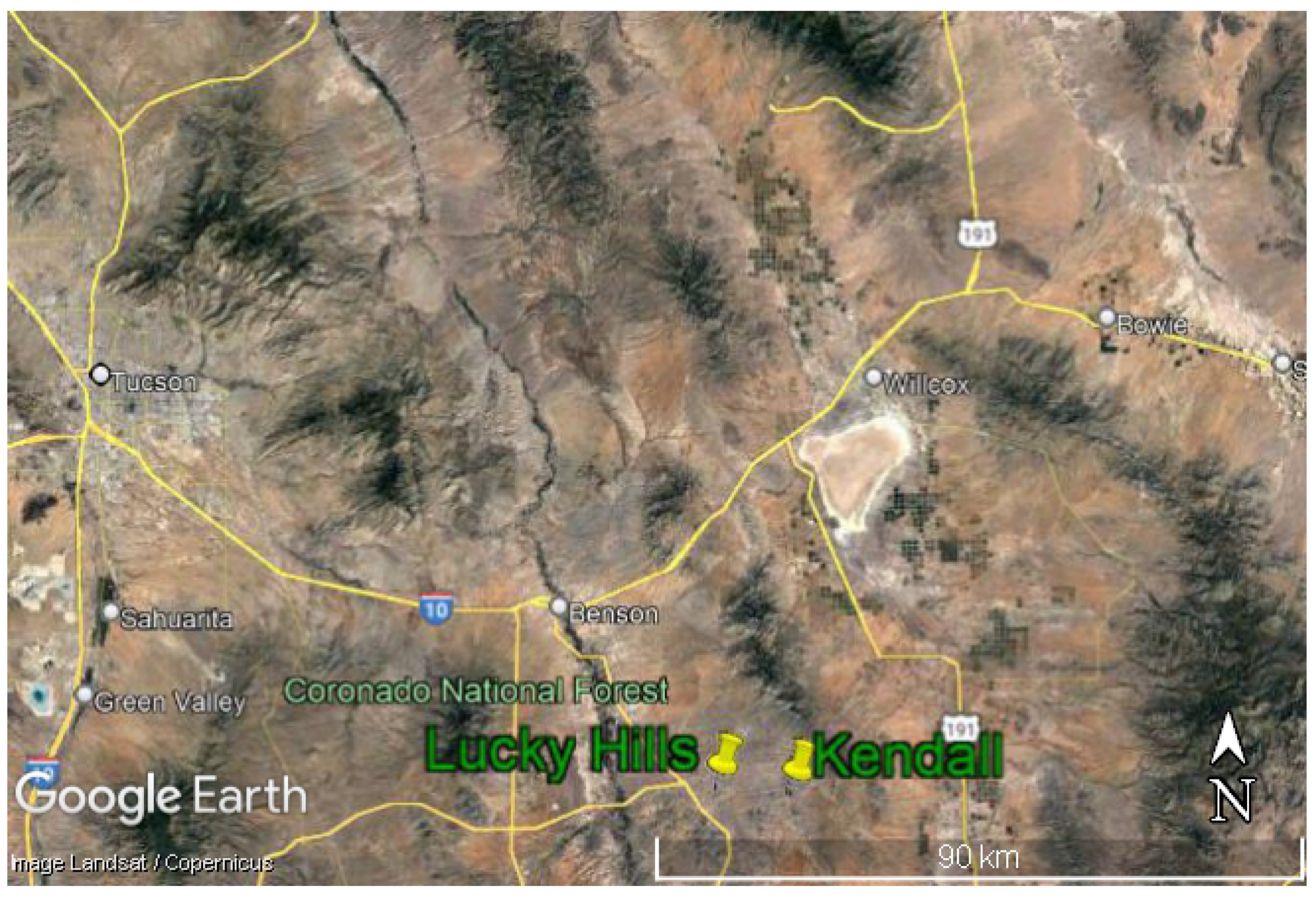
3.1.1. Walnut Gulch (WG)

This area is located near the town of Tombstone in southeastern Arizona, USA. There are two sites in this area: Kendall and Lucky Hills. These sites are within the Walnut Gulch Experimental Watershed [24]. Figure 1 shows the location of the sites. The Kendall site has nine nodes, and the Lucky Hills site has seven nodes. The in situ sensors at each node are installed at depths of 5 cm, 15 cm, 30 cm, and 50 cm. In 2015, the sensors were installed, and the site was operational until Oct 2019. After a hiatus during the COVID-19 pandemic, the site was revived in August 2022.

These sites are relatively dry all year round except in the monsoon season, which is usually in July, August, and the first half of September [25]. Thus, high vegetation water content (VWC) is expected during the monsoon season. Figure 2a,b show photos of the area during the dry season and the monsoon season, respectively, highlighting the presence of green vegetation during the latter.

To account for the presence of vegetation, an attenuation factor was applied to ${\sigma }_0$. This is based on the vegetation model of [26] (Equation (11.4)). The normalized BRCS with vegetation is expressed as

$${\sigma }_{0,\mathrm{VEG}}\left(\overrightarrow{\rho }\right)=exp\left[-{\kappa }^{p}dsec\left({\theta }_{\mathrm{i}}\right)\right]exp\left[-{\kappa }^{q}dsec\left({\theta }_{\mathrm{s}}\right)\right]{\sigma }_0\left(\overrightarrow{\rho }\right)$$

(21)

where ${\kappa }^{p,q}$ is the p,q-polarized extinction coefficient ($p,q\in \{v,h,l,r\}$), d is the vegetation depth, ${\theta }_{\mathrm{i}}$ is the local incidence angle, and ${\theta }_{\mathrm{s}}$ is the local scattering angle. We refer to the model with this feature as IGOT-VEG. It is worth noting that when d or $\kappa$ is zero, the IGOT-VEG reduces to the IGOT model.

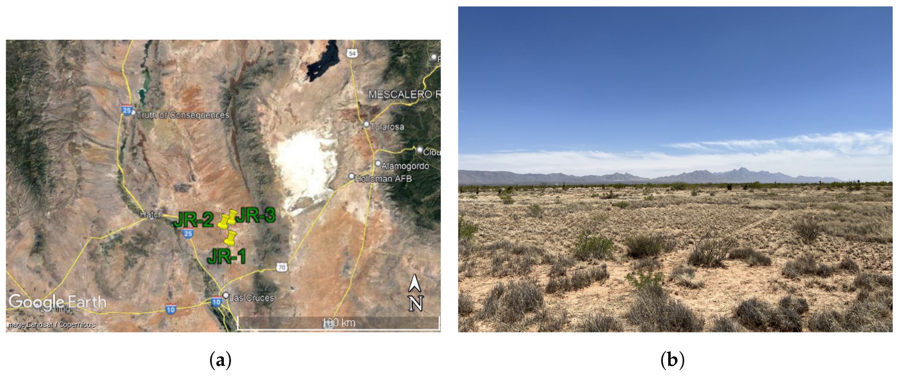
3.1.2. Jornada Experimental Range (JER)

This area is located to the southwest of the White Sands National Park, NM, USA. There are three SoilSCAPE sites in this area, denoted as JR-1, JR-2, and JR-3. Figure 3a shows the location of the sites on a satellite map. The sites are within the Jornada Experimental Range [27].

In each site, four nodes are equipped with four soil moisture sensors installed at 5 cm, 10 cm, 20 cm, and 30 cm depths. Sensors were installed in May 2022. Node JR-3-3 of the JR-3 site is located within 100 m of the US Climate Reference Network (USCRN) Las Cruces station [28]. These sites are mostly dry with minimal vegetation.

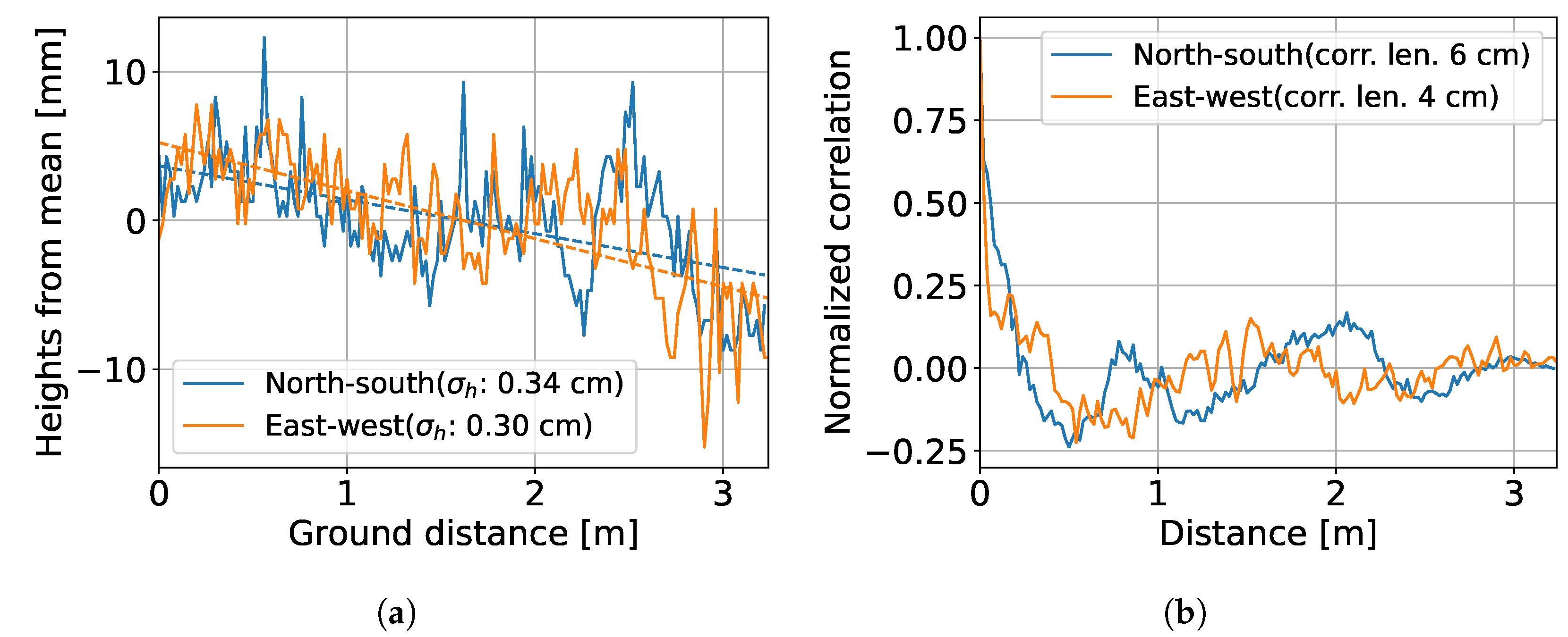
3.2. Surface Roughness Measurements

The small-scale surface roughness ${\sigma }_{\mathrm{S}}$ was estimated using manual in situ measurements. These measurements were performed using a laser range finder mounted on a spirit level supported by two tripods, as shown in Figure 4.

The measurement was made by first leveling the spirit level about both horizontal axes (pitch and roll). Second, the height to the ground surface was measured every 2 cm. The level is about 120 cm long; therefore, the measurement was repeated three times to obtain a larger baseline. This procedure was performed in both the north–south and the east–west direction. During the measurements, special care was taken to avoid measuring vegetation height instead of ground surface height. The surface roughness was calculated by first calculating the height values relative to the surface slope line. Then, the root mean square (RMS) surface roughness was calculated. The slope line was assumed to be captured by the DEM.

A roughness measurement was taken at each site using a baseline close to 3 m. Thus, three roughness measurements were taken in the JER area, and two measurements were taken in the WG area. The roughness measurements at JER were taken in May 2022, and the measurements at WG were taken in August 2022.

The surface height measurements and the surface correlation of the measurement at site JR-1 are shown in Figure 5. The dashed lines in Figure 5a are the surface slope lines. The RMS roughness ${\sigma }_{\mathrm{h}}$ and the surface correlation length of the WG and JER sites are given in

Table 1. Calculated surface roughness and surface correlation lengths for JER and WG sites based on laser range-finder measurements.

Location	Orientation	${\mathit{\sigma }}_{\mathbf{h}}$ [cm]	Correlation Length [cm]	Correlation Length/${\mathit{\sigma }}_{\mathbf{h}}$
JR-1	N-S	0.34	6	17.8
	E-W	0.30	4	13.1
JR-2	N-S	0.56	16	28.7
	E-W	0.56	26	46.7
JR-3	N-S	1.44	26	18.0
	E-W	0.67	6	8.9
KN	N-S	0.73	4	5.5
	E-W	0.46	2	4.3
LH	N-S	0.88	4	4.5
	E-W	0.34	2	5.8

. The roughness measurements at the WG sites were taken in the flat area within the sites. Moreover, the location of the measurements was in an area with lower vegetation to facilitate the measurement. Some data points in the measurement at the Kendall site were skipped due to vegetation. Thus, the roughness measurements of WG sites are believed to be lower than the mean RMS surface roughness.

For the wavelength of the GPS L1 signal, these in situ measurements can be used to estimate the characteristics of the surface height in the spatial domain from a fraction of a wavelength to a few wavelengths. This makes the in situ measurements more suited for estimating the small-scale roughness of the IGOT model. Since the in situ roughness measurements were sparse and did not capture the heterogeneity of the sites, the in situ measurements guided the selection of the small-scale roughness parameter ${\sigma }_{\mathrm{S}}$.

3.3. CYGNSS and Ancillary Data

CYGNSS is a National Aeronautics and Space Administration (NASA) mission consisting of eight low-Earth orbit satellites for GNSS-R [7]. Each satellite has two off-nadir antennas for science measurements and a zenith antenna for navigation and receiving the direct GPS signal. CYGNSS satellites generate DDMs from GPS L1 signals. The mission was originally designed to estimate wind speed over the ocean. However, after launch, it has been utilized for other applications, including soil moisture estimation. In this work, we used the CYGNSS L1 v3.1 product [29].

The one-arc-second SRTM DEM [30] was used in the IGOT model as ${\zeta }_{\mathrm{DEM}}$. Furthermore, the DEM gradient was calculated using the method presented in [31], which calculates the gradient of each pixel in the DEM by fitting a plane using a window of a specific size. This method was used to reduce the noise in the DEM gradient. The window size in this work has units of DEM samples, each of which is approximately 30 m in extent.

4. Validation Results

In this section, the IGOT model is validated using four tracks: the first and second tracks are over the WG area, and the last two are over the JER sites. The peak reflectivity of these tracks is studied, and three full DDMs from the tracks are analyzed. In situ soil moisture measurements at 5 cm depth are used in the IGOT model. Specifically, the spatially averaged soil moisture value from all the available nodes is used.

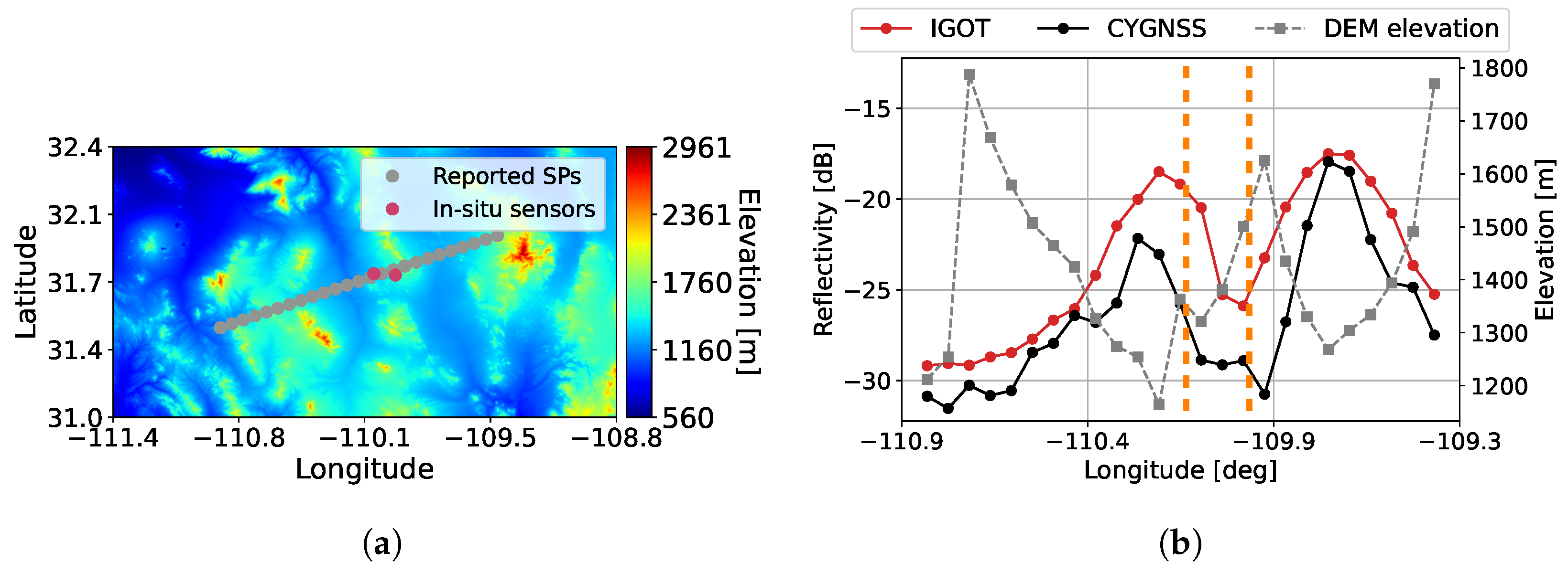
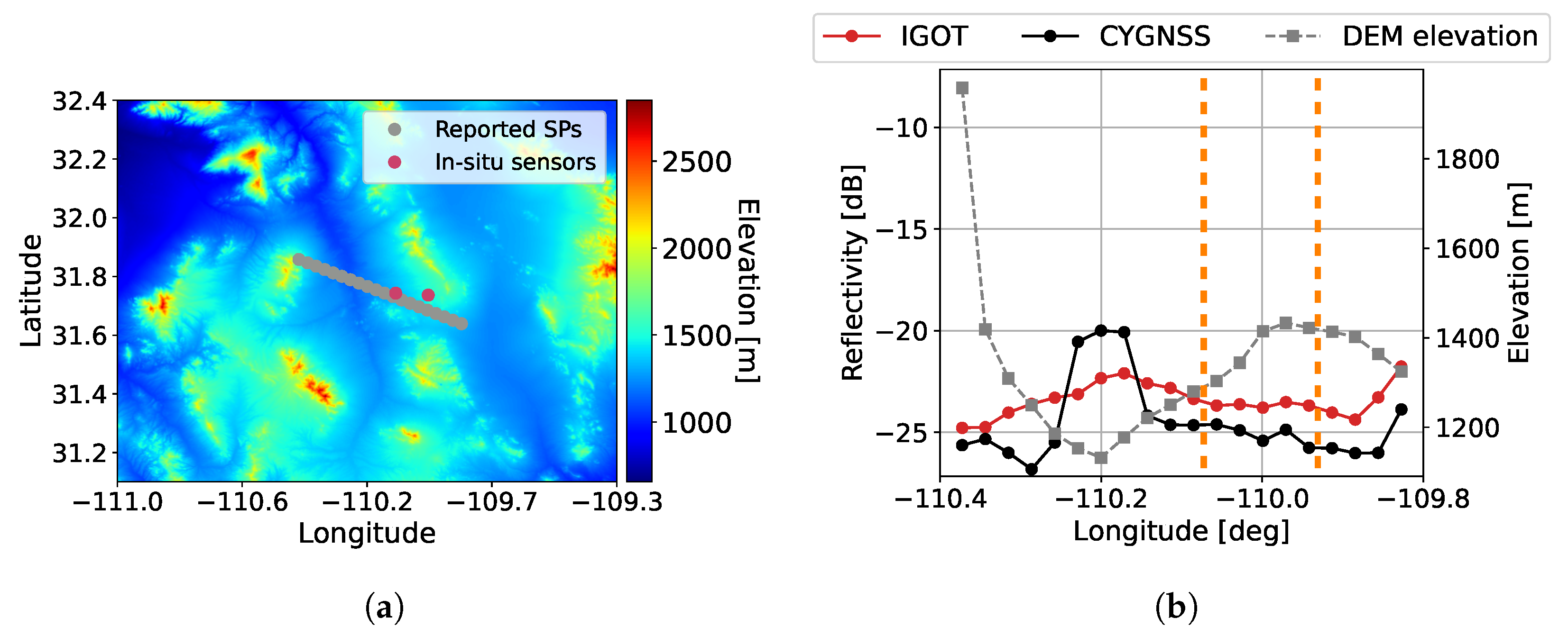
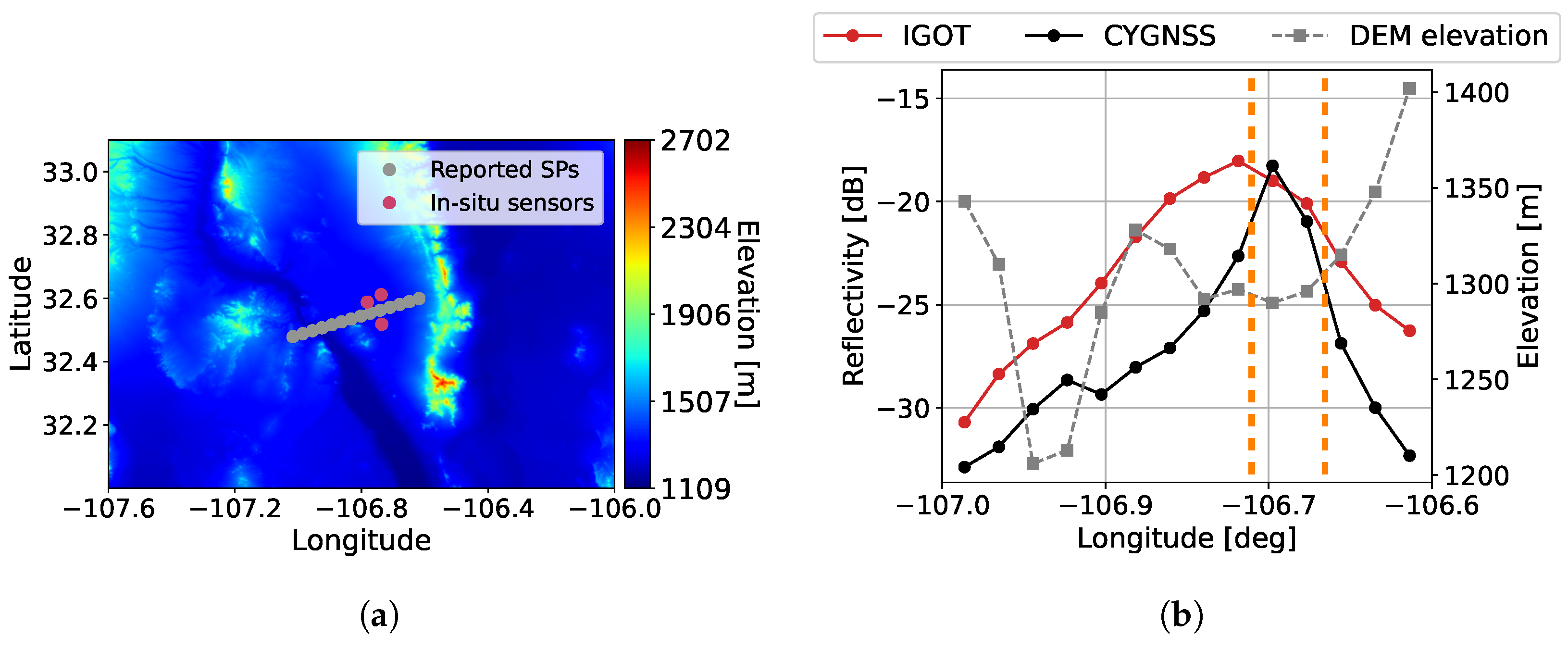
4.1. Along-Track Results

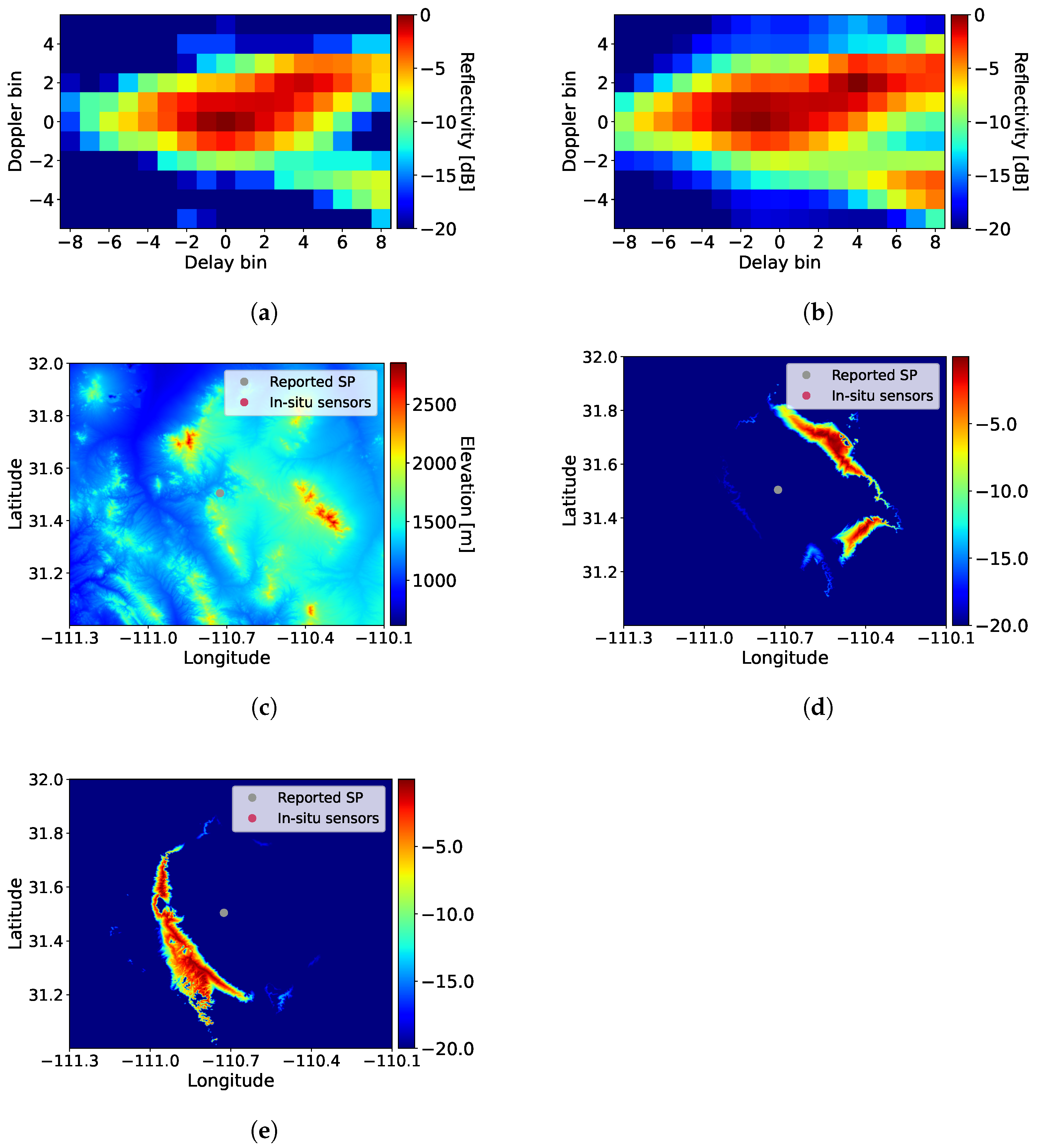
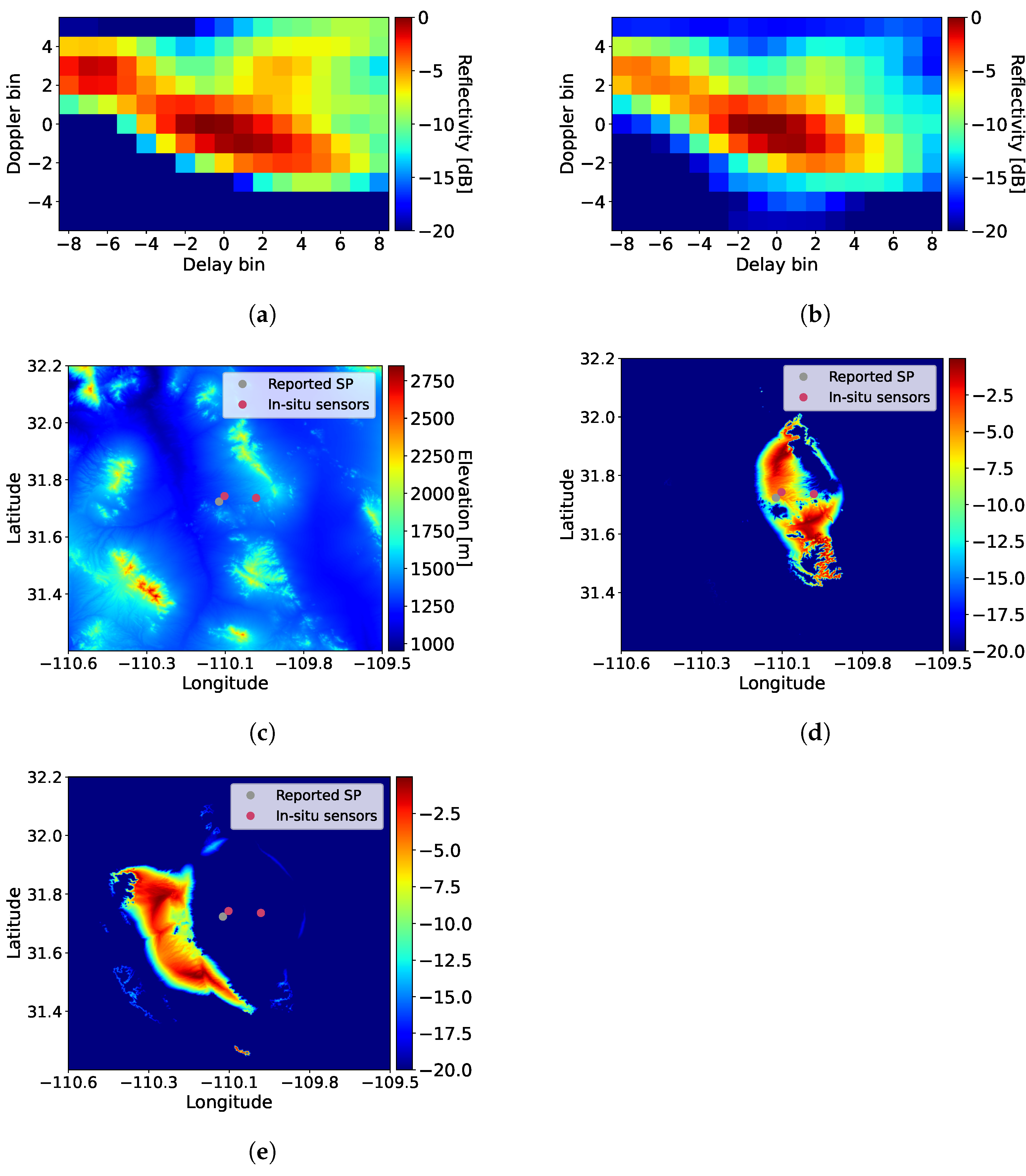
The first and second tracks over the WG area were acquired on 2019-02-05 and 2019-09-15, respectively. The second track was during the monsoon season. Thus, a higher VWC is expected. At the time of the first track, the in situ soil moisture was 0.18 m³ m⁻³. For the second track, the in situ soil moisture was 0.51 m³ m⁻³, which is the saturation level. In the model, the soil clay percentage was set to 20%, and the DEM window size was set to nine samples for both tracks. Furthermore, the parameter ${\sigma }_L$ of Equation (19) was set to 0.4° for both tracks. Selection of the previous two parameters was made empirically and acknowledging the fact that this area has rough topography. Moreover, the small-scale roughness ${\sigma }_S$ was set to 1.25 cm, which is higher than the in situ measurements, but within the IGOT model validity. We expect the surface roughness to be higher than the in situ measurements, as the measurements were taken in a low relief area of the sites. Finally, the vegetation optical depth of the first track was zero, as we expected the vegetation to be dry. On the other hand, the vegetation parameter $\kappa d$ of the second track was set to $0.2$. This value was selected empirically to match CYGNSS reflectivity. All of the model parameters and the track information are summarized in

Table 2. Analyzed track information.

	WG Track 1	WG Track 2	JER Track 1	JER Track 2
Date	5 February 2019	15 September 2019	30 May 2022	30 May 2022
Time [UTC]	19:41	14:31	14:27	17:57
Spacecraft ID	8	6	4	5
Channel number	4	4	3	4
Starting sample ID	70,680	104,540	10,419	128,830
Number of DDM	25	20	14	18
SNR range [dB]	4–13	5–10	2–10	2–10
Soil moisture [m3 m−3]	0.18	0.51 *	0.01	0.01
Soil clay percentage	20%	20%	20%	20%
${\sigma }_L$	0.4°	0.4°	0.1°	0.1°
${\sigma }_S$ [cm]	1.25	1.25	1.25	1.25
DEM window size	9	9	15	15
$\kappa d$	0	0.2	0	0

* Saturated soil moisture.

.

The WG track 1 SP and the in situ sensor locations are shown in Figure 6a. The peak reflectivity of both CYGNSS and IGOT is shown in Figure 6b. In the figure, the points between the two vertical orange lines are between the SoilSCAPE sites. As illustrated in the figure, the IGOT model reflectivity follows the CYGNSS reflectivity for most of the points on the track. Furthermore, the median difference between CYGNSS reflectivity and IGOT reflectivity is about 2.5 dB. An anticorrelation relation between the elevation and peak reflectivity of both the IGOT model and CYGNSS can be observed in Figure 6b. This is mainly due to the fact that the valley basins are smoother than the hills in this region, which results in higher reflectivity in the valleys.

The WG track 2 SP and the in situ sensor locations are shown in Figure 7a. The peak reflectivity is shown in Figure 7b. As illustrated in the figure, the peak reflectivity of the IGOT-VEG model matches the CYGNSS reflectivity with good accuracy except for three DDMs. These DDMs lie between −110.25° and −110.4° longitudes, as shown in Figure 7a. For all peak reflectivity points on the track, the median value of the difference between CYGNSS and IGOT-VEG reflectivity is about 1.8 dB. The three outlier DDMs, which IGOT-VEG underestimated, are over the San Pedro river. This river could be the reason for the high CYGNSS reflectivity, as the high water level of the river during the monsoon season can cause strong coherent reflections and increase the DDM reflectivity, which is not accounted for in the parameterization of the IGOT model.

The two tracks over JER were acquired within four hours of each other on 30 May 2022. Selection of the track length was made such that the DDM signal-to-noise ratio (SNR) is equal to or over 2 dB. All the DDMs in these tracks have an SNR between 2 dB and 10 dB. During these tracks, the in situ soil moisture was about 0.01 m³ m⁻³, which is very dry. In the model, the soil clay percentage was set to 20%, and ${\sigma }_L$ was set to be 0.1°. The latter is lower than the value used for the WG tracks as this area is expected to have less topography, as illustrated in the elevation maps of Figure 8a and Figure 9a. The small-scale roughness ${\sigma }_S$ was set to 1.25 cm, which is close to the highest in situ roughness measurement. In the model, the DEM window size was set to 15 samples, which is larger than the value used for the WG tracks. The DEM window size was increased to reduce the DEM noise, as the JER area is relatively flat compared to the WG area. All of the JER tracks used the same IGOT parameters. A summary of these parameters and the track information is provided in Table 2.

The JER track 1 peak reflectivity of each of CYGNSS and the IGOT model is shown in Figure 8b, which shows that the reflectivity of the IGOT model follows the CYGNSS reflectivity. Furthermore, the median difference of reflectivity between CYGNSS and IGOT is about 4 dB.

For JER track 2, the peak reflectivity of each of CYGNSS and the IGOT model is shown in Figure 9b. The median difference of reflectivity between CYGNSS and IGOT is about 4 dB. For most of the DDMs, the IGOT model reflectivity follows the CYGNSS reflectivity. However, there is a jump in CYGNSS reflectivity of the DDM with a longitude of −107.01° that the IGOT model did not capture. This increase in CYGNSS reflectivity may be due to a vertically variable soil moisture profile that is wetter beneath the surface since the SP of this DDM is located in a valley, as shown in Figure 9.

4.2. DDM Results

In this section, an analysis of three DDMs is presented. Two DDMs are from WG track 1, and the last is from JER track 1. These DDMs were selected based on their proximity to the in situ sensors and distinct features.

The first DDM is sample 70,682 of WG track 1, the third sample from the west. The SP is located at a latitude of 31.505° and longitude of −110.726° which is west of the in situ sensors. Figure 10a,b show the normalized CYGNSS DDM and the normalized DDM estimated by the IGOT model, respectively. Furthermore, the elevation map of the area around the SP is shown in Figure 10c. As shown in Figure 10a, this DDM has a strong positive Doppler tail. Despite the complex shape of this DDM, the IGOT model is able to estimate the CYGNSS DDM with good accuracy, which includes generating the DDM horseshoe shape, as illustrated in Figure 10b. However, the intensity of the horseshoe is not captured fully by the model. The IGOT model has the capability of plotting the WAF projection of a specific DDM cell. Two cells within the horseshoe shape are of interest. The first is (4, 2), where the reflectivity of this cell is close to the SP reflectivity. The WAF projection of this cell is shown in Figure 10d, which illustrates that the majority of the energy of this cell is from the valleys. The second cell is (8, −3), which was selected due to the relative reflectivity discrepancies between CYGNSS and IGOT. As illustrated in Figure 10e, the majority of the cell energy is from a valley.

The second DDM is sample 70,693 of WG track 1, the closest DDM to the Lucky Hills site from the west. This DDM SP is located at 31.724° latitude and −110.072° longitude, with a reported SNR of 5.5 dB. Furthermore, the normalized reflectivities of the CYGNSS DDM and the IGOT model DDM are shown in Figure 11a,b, respectively. Moreover, the elevation map of the area close to the SP location is shown in Figure 11c. This DDM has non-zero cells in the negative delay. In a DDM, no return is expected before the SP. To understand this phenomenon, the WAF projection of cell (−7, 3) was examined, the cell that has the highest reflectivity in the negative delay part of the DDM. The WAF projection of this cell is presented in Figure 11d. It shows that the cell scattering area is around the CYGNSS reported SP location. On the other hand, the WAF projection of the DDM SP (0, 0) shows that its scattering area is on the west side of the reported SP location, as shown in Figure 11e. This DDM has two strong scattering areas, where the DDM is centered on the strongest. The first scattering area is associated with the reported SP location, which contains the valley, as shown in Figure 11d. The other scattering area is associated with the high elevation area and its slope, as shown in Figure 11e.

The third DDM is sample 104,027 of JER track 1. Its SP is located at 32.553° latitude and −106.771° longitude with an SNR of 8.7 dB. This DDM was selected due to its proximity to the in situ sensors and the SP footprint location. Figure 12d shows the elevation map of the area around the SP. Furthermore, the normalized CYGNSS DDM and IGOT model DDM are presented in Figure 12a,b, respectively. These figures show that the DDM of the IGOT model has a similar shape as the CYGNSS DDM. Furthermore, the WAF projection map of the SP matches the expected shape of a flat region, as shown in Figure 12c. A WAF projection map of a SP of a flat area is expected to have an elliptical shape.

5. Discussion and Future Directions

The IGOT model has been validated with CYGNSS data over three areas: WG, JER, and SLV. In Section 4, the results of WG and JER were presented. Furthermore, the results of SLV were discussed in [20]. These sites cover various topographies from rough (WG) to smooth (JER). The results show that this model can estimate CYGNSS DDMs with good accuracy under most conditions. Both the peak reflectivity and the DDM shape of the IGOT model were close to that of CYGNSS with discrepancies in some of the points that are discussed in this section. The performance assessment criteria we follow are that (1) the shape of the modeled DDM should track the observed one, and (2) the values of reflectivity should be within a few dB of the measured ones. Some of the latter may be accounted for based on the calibration accuracy of CYGNSS land DDMs, and some of it can be accounted for based on the uncertainties of input parameters.

The discrepancies of some of the points in the tracks can be attributed to the SRTM noise and vertical resolution, as the model is sensitive to DEMs. In generating the IGOT DDMs, we assumed that both ${\sigma }_L$ and ${\sigma }_S$ are fixed for the whole area. Hence, we selected one value for WG sites and another value for JER sites. This assumption was made due to limited information on these parameters. However, in reality, these parameters are not constant. Thus, some of the errors in peak reflectivity are also attributed to this assumption. Using a lidar DEM instead of the SRTM DEM can improve the match between CYGNSS reflectivity and IGOT reflectivity, as proven in [31].

The results of the WG tracks, demonstrated in Figure 6 and Figure 7, show the importance of accounting for VWC in modeling GNSS-R. In this paper, the vegetation modeling is simple and can be applied to low-vegetated terrains. To account for dense vegetation, including forests, an advanced electromagnetic model is required as the scattering from the vegetation components is not negligible. An adaptation of the model presented in [32] to GNSS-R can be used to improve the IGOT model to account for dense vegetation and is the subject of our ongoing work.

The results of JER track 2 highlight a limitation of the IGOT model. Specifically, the jump in reflectivity of the DDM located at 32.59° latitude and −107.01° longitude (Figure 9b) is expected to be due to the presence of higher moisture content in subsurface soil, as the dry surface soil allows for deep penetration of the GPS L1 signal. However, the model used in this work only accounts for surface reflection. Thus, a modification to the Fresnel reflection coefficient $\mathcal{R}$ is needed to model the reflections from a subsurface soil moisture profile. We expect the subsurface soil moisture to affect the DDM reflectivity when the surface soil is very dry. However, the contribution of subsurface soil dielectric constant change to the Fresnel reflection coefficient for the frequency of the GPS L1 signal is expected to be negligible when the surface soil moisture is high.

The DDM results, presented in Figure 10, Figure 11 and Figure 12, give insight into the location and area of the DDM cells. Furthermore, the DDM of Figure 11 shows a case where the SP location was changed due to topography. In this DDM (Second DDM), there are two strong returns at (0, 0) and (−7, 3). The strongest is at (0, 0). However, it does not correspond to the reported SP location, as shown in Figure 11e. Instead, the scattering is from the high elevation area and its slope.

The discrepancies in relative reflectivity between CYGNSS and IGOT in the tail of the first DDM, shown in Figure 10, can be attributed to heterogeneity in the surface roughness of the scattering regions. These scattering regions are valleys as illustrated in Figure 10d,e. Although the random roughness scales in the IGOT model can vary spatially, in this work, we fixed the value due to a lack of spatial information on these roughness scales. Another possible reason for the discrepancies is the presence of fading effects due to this random roughness that our incoherent model failed to capture [33].

The cutoff wavenumber between the short-scale and the long-scale component of the IGOT model needs to be such that the assumptions made in Section 2.1 are valid. Specifically, the long-scale component is smooth relative to the wavenumber and the short-scale component has a narrow correlation function. In ocean application, this cutoff was selected between $k/6$ and $k/3$ [22], depending on the wind speed. In [34], the cutoff was selected to be $3k{\left({\sigma }_X{\sigma }_Y\right)}^{1/2}$, where ${\sigma }_X$ and ${\sigma }_Y$ are the standard deviations of the long-scale component in the x and y directions, respectively. The model in [34] was developed for both ocean and land applications, and the cutoff wavenumber was selected to ensure a smooth transition between the two scales and the constraints of each component.

In validating the IGOT model, both ${\sigma }_L$ and ${\sigma }_S$ were fixed to a single value for each area. However, these parameters can vary spatially. Varying ${\sigma }_L$ was explored in [31] by estimating the parameter from lidar measurements with 30 cm spatial resolution. The results showed that estimating ${\sigma }_L$ from lidar can improve the matching with CYGNSS observations. In theory, ${\sigma }_S$ can also be estimated from lidar for some surfaces. For surfaces with known spectral shapes, the spectra of the surface can be estimated from the lidar measurements. Then, ${\sigma }_S$ can be estimated from the area of the spectra within the small-scale roughness region.

The JER DDM presented in Figure 12 resembles a land DDM from flat regions. Thus, the WAF projection of the SP has an almost convex shape, as shown in Figure 12c. These DDM properties are the result of the special characteristics of this area. The JER sites are located in a relatively flat region with minimal vegetation and almost homogeneous soil moisture. Thus, the IGOT model can potentially assist in validating the CYGNSS calibration over land and other systems in the future. However, a lidar DEM needs to be used instead of the SRTM DEM to reduce the DEM noise. It should be noted that the validation should be restricted to the DDMs located in the flat area and not the full extent of the analyzed JER tracks.

This model can be used in a physics-based soil moisture retrieval method to estimate the surface soil moisture value from CYGNSS observation(s). Such a method was presented in [35], which used a global optimizer and a forward model to estimate soil moisture from CYGNSS DDMs. However, unlike the IGOT model, the forward model in [35] can be applied to flat terrains only. Thus, by replacing the model in [35] with the IGOT model, the retrieval method can be extended to retrieve soil moisture value from areas with topography.

Studying the sensitivity of the IGOT model to noise and errors in its input parameters and their implications on soil moisture retrievals is essential for estimating the performance of using the IGOT model for retrievals.

6. Conclusions

This paper presented a GNSS-R model, which was validated with CYGNSS DDMs over two areas. The peak reflectivity of four tracks over the validation sites was studied. Additionally, three full DDMs from the studied tracks were presented with WAF projection maps for some of the DDM cells. The IGOT model results matched CYGNSS with good accuracy under most conditions, in both peak reflectivity and the DDM shape. For the studied tracks, the average error in peak reflectivity was between 1 dB and 4 dB. The model of this paper increases the fidelity of GNSS-R signal modeling for land applications.

References

1. Gleason, S.; Hodgart, S.; Yiping, S.; Gommenginger, C.; Mackin, S.; Adjrad, M.; Unwin, M. Detection and Processing of Bistatically Reflected GPS Signals from Low Earth Orbit for the Purpose of Ocean Remote Sensing. IEEE Trans. Geosci. Remote Sens. 2005, 43, 1229–1241. [Google Scholar] [CrossRef] [Green Version]
2. Unwin, M.; Duncan, S.; Jales, P.; Blunt, P.; Tye, J. Implementing GNSS-Reflectometry in Space on the TechDemoSat-1 Mission. In Proceedings of the 27th International Technical Meeting of the Satellite Division of The Institute of Navigation (ION GNSS+ 2014), Tampa, FL, USA, 8–12 September 2014; pp. 1222–1235. [Google Scholar]
3. Ruf, C.S.; Gleason, S.; Jelenak, Z.; Katzberg, S.; Ridley, A.; Rose, R.; Scherrer, J.; Zavorotny, V. The CYGNSS Nanosatellite Constellation Hurricane Mission. In Proceedings of the International Geoscience and Remote Sensing Symposium (IGARSS), Munich, Germany, 22–27 July 2012; pp. 214–216. [Google Scholar] [CrossRef]
4. Munoz-Martin, J.F.; Fernandez, L.; Perez, A.; Ruiz-De-azua, J.A.; Park, H.; Camps, A.; Domínguez, B.C.; Pastena, M. In-Orbit Validation of the FMPL-2 Instrument—The GNSS-R and L-Band Microwave Radiometer Payload of the FSSCat Mission. Remote Sens. 2020, 13, 121. [Google Scholar] [CrossRef]
5. Freeman, V.; Masters, D.; Jales, P.; Esterhuizen, S.; Ebrahimi, E.; Irisov, V.; Khadhra, K.B. Earth Surface Monitoring with Spire’s New GNSS Reflectometry (GNSS-R) CubeSats. In Proceedings of the EGU General Assembly 2020, Online, 4–8 May 2020. EGU2020-13766. [Google Scholar] [CrossRef]
6. Jing, C.; Niu, X.; Duan, C.; Lu, F.; Di, G.; Yang, X. Sea Surface Wind Speed Retrieval from the First Chinese GNSS-R Mission: Technique and Preliminary Results. Remote Sens. 2019, 11, 3013. [Google Scholar] [CrossRef] [Green Version]
7. Ruf, C.S.; Chew, C.; Lang, T.; Morris, M.G.; Nave, K.; Ridley, A.; Balasubramaniam, R. A New Paradigm in Earth Environmental Monitoring with the CYGNSS Small Satellite Constellation. Sci. Rep. 2018, 8, 1–13. [Google Scholar] [CrossRef] [Green Version]
8. Wan, W.; Liu, B.; Zeng, Z.; Chen, X.; Wu, G.; Xu, L.; Chen, X.; Hong, Y. Using CYGNSS Data to Monitor China’s Flood Inundation during Typhoon and Extreme Precipitation Events in 2017. Remote Sens. 2019, 11, 854. [Google Scholar] [CrossRef] [Green Version]
9. Chew, C.; Small, E. Description of the UCAR/CU Soil Moisture Product. Remote Sens. 2020, 12, 1558. [Google Scholar] [CrossRef]
10. Wu, X.; Ma, W.; Xia, J.; Bai, W.; Jin, S.; Calabia, A. Spaceborne GNSS-R Soil Moisture Retrieval: Status, Development Opportunities, and Challenges. Remote Sens. 2020, 13, 45. [Google Scholar] [CrossRef]
11. Campbell, J.D.; Melebari, A.; Moghaddam, M. Modeling the Effects of Topography on Delay-Doppler Maps. IEEE J. Sel. Top. Appl. Earth Obs. Remote Sens. 2020, 13, 1740–1751. [Google Scholar] [CrossRef]
12. Dente, L.; Guerriero, L.; Comite, D.; Pierdicca, N. Space-Borne GNSS-R Signal over a Complex Topography: Modeling and Validation. IEEE J. Sel. Top. Appl. Earth Obs. Remote Sens. 2020, 13, 1218–1233. [Google Scholar] [CrossRef]
13. Comite, D.; Ticconi, F.; Dente, L.; Guerriero, L.; Pierdicca, N. Bistatic Coherent Scattering from Rough Soils with Application to GNSS Reflectometry. IEEE Trans. Geosci. Remote Sens. 2020, 58, 612–625. [Google Scholar] [CrossRef]
14. Zhu, J.; Tsang, L.; Xu, H. A Physical Patch Model for GNSS-R Land Applications. Prog. Electromagn. Res. 2019, 165, 93–105. [Google Scholar] [CrossRef] [Green Version]
15. Zavorotny, V.U.; Voronovich, A.G. Scattering of GPS Signals from the Ocean with Wind Remote Sensing Application. IEEE Trans. Geosci. Remote Sens. 2000, 38, 951–964. [Google Scholar] [CrossRef] [Green Version]
16. Zavorotny, V.U.; Larson, K.M.; Braun, J.J.; Small, E.E.; Gutmann, E.D.; Bilich, A.L. A Physical Model for GPS Multipath Caused by Land Reflections: Toward Bare Soil Moisture Retrievals. IEEE J. Sel. Top. Appl. Earth Obs. Remote Sens. 2010, 3, 100–110. [Google Scholar] [CrossRef]
17. Ren, B.; Zhu, J.; Tsang, L.; Xu, H. Analytical Kirchhoff Solutions (AKS) and Numerical Kirchhoff Approach (NKA) for First-Principle Calculations of Coherent Waves and Incoherent Waves at P Band and L Band in Signals of Opportunity (SoOp). Prog. Electromagn. Res. 2021, 171, 35–73. [Google Scholar] [CrossRef]
18. Kurum, M.; Deshpande, M.; Joseph, A.T.; O’Neill, P.E.; Lang, R.H.; Eroglu, O. SCoBi-Veg: A Generalized Bistatic Scattering Model of Reflectometry From Vegetation for Signals of Opportunity Applications. IEEE Trans. Geosci. Remote Sens. 2019, 57, 1049–1068. [Google Scholar] [CrossRef]
19. Park, H.; Camps, A.; Castellvi, J.; Muro, J. Generic Performance Simulator of Spaceborne GNSS-Reflectometer for Land Applications. IEEE J. Sel. Top. Appl. Earth Obs. Remote Sens. 2020, 13, 3179–3191. [Google Scholar] [CrossRef]
20. Campbell, J.D.; Akbar, R.; Bringer, A.; Comite, D.; Dente, L.; Gleason, S.T.; Guerriero, L.; Hodges, E.; Johnson, J.T.; Kim, S.B.; et al. Intercomparison of Electromagnetic Scattering Models for Delay-Doppler Maps along a CYGNSS Land Track with Topography. IEEE Trans. Geosci. Remote Sens. 2022, 60, 1–13. [Google Scholar] [CrossRef]
21. Akbar, R.; Campbell, J.; Silva, A.R.; Chen, R.; Melebari, A.; Hodges, E.; Entekhabi, D.; Ruf, C.; Moghaddam, M. SoilSCAPE Wireless in Situ Networks in Support of CYGNSS Land Applications. In Proceedings of the IGARSS 2020–2020 IEEE International Geoscience and Remote Sensing Symposium, Waikoloa, HI, USA, 26 September–2 October 2020; pp. 5042–5044. [Google Scholar] [CrossRef]
22. Thompson, D.; Elfouhaily, T.; Garrison, J. An Improved Geometrical Optics Model for Bistatic GPS Scattering from the Ocean Surface. IEEE Trans. Geosci. Remote Sens. 2005, 43, 2810–2821. [Google Scholar] [CrossRef]
23. Pascual, D.; Park, H.; Camps, A.; Arroyo, A.A.; Onrubia, R. Simulation and Analysis of GNSS-R Composite Waveforms Using GPS and Galileo Signals. IEEE J. Sel. Top. Appl. Earth Obs. Remote Sens. 2014, 7, 1461–1468. [Google Scholar] [CrossRef]
24. Goodrich, D.C.; Keefer, T.O.; Unkrich, C.L.; Nichols, M.H.; Osborn, H.B.; Stone, J.J.; Smith, J.R. Long-Term Precipitation Database, Walnut Gulch Experimental Watershed, Arizona, United States. Water Resour. Res. 2008, 44, 5. [Google Scholar] [CrossRef]
25. Osborn, H.B. Persistence of Summer Rainy and Drought Periods on a Semiarid Rangeland Watershed. Int. Assoc. Sci. Hydrol. Bull. 1968, 13, 14–19. [Google Scholar] [CrossRef]
26. Ulaby, F.T.; Long, D.G. Microwave Radar and Radiometric Remote Sensing; The University of Michigan Press: Ann Arbor, MI, USA, 2015; pp. 1–1116. [Google Scholar]
27. Havstad, K.M.; Huenneke, L.F.; Schlesinger, W.H. Structure and Function of a Chihuahuan Desert Ecosystem: The Jornada Basin Long-Term Ecological Research Site; Oxford University Press: Oxford, UK, 2006. [Google Scholar] [CrossRef]
28. Diamond, H.J.; Karl, T.R.; Palecki, M.A.; Baker, C.B.; Bell, J.E.; Leeper, R.D.; Easterling, D.R.; Lawrimore, J.H.; Meyers, T.P.; Helfert, M.R.; et al. U.S. Climate Reference Network After One Decade of Operations Status and Assessment. Bull. Am. Meteorol. Soc. 2013, 94, 485–498. [Google Scholar] [CrossRef]
29. CYGNSS. CYGNSS Level 1 Science Data Record Version 3.1; Dataset; PO.DAAC: Pasadena, CA, USA, 2021. Available online: https://podaac.jpl.nasa.gov/dataset/CYGNSS_L1_V3.1 (accessed on 15 January 2023).
30. Earth Resources Observation and Science (EROS) Center. Shuttle Radar Topography Mission 1 Arc-Second Global; U.S. Geological Survey: Reston, VA, USA, 2018. [CrossRef]
31. Hodges, E.; Campbell, J.D.; Melebari, A.; Bringer, A.; Johnson, J.T.; Moghaddam, M. Using Lidar Digital Elevation Models for Reflectometry Land Applications. IEEE Trans. Geosci. Remote Sens. 2023, 12, 2308. [Google Scholar] [CrossRef]
32. Burgin, M.S.; Khankhoje, U.K.; Duan, X.; Moghaddam, M. Generalized Terrain Topography in Radar Scattering Models. IEEE Trans. Geosci. Remote Sens. 2016, 54, 3944–3952. [Google Scholar] [CrossRef]
33. Comite, D.; Pierdicca, N. Decorrelation of the Near-Specular Scattering in GNSS Reflectometry from Space. IEEE Trans. Geosci. Remote Sens. 2022, 60, 2005213. [Google Scholar] [CrossRef]
34. DI Martino, G.; DI Simone, A.; Iodice, A.; Riccio, D. Bistatic Scattering from Anisotropic Rough Surfaces via a Closed-Form Two-Scale Model. IEEE Trans. Geosci. Remote Sens. 2021, 59, 3656–3671. [Google Scholar] [CrossRef]
35. Azemati, A.; Melebari, A.; Campbell, J.D.; Walker, J.P.; Moghaddam, M. GNSS-R Soil Moisture Retrieval for Flat Vegetated Surfaces Using a Physics-Based Bistatic Scattering Model and Hybrid Global/Local Optimization. Remote Sens. 2022, 14, 3129. [Google Scholar] [CrossRef]
Figure 1. Satellite map of WG SoilSCAPE sites.
Remotesensing 15 01880 g001
Figure 2. Photos of WG taken in the dry season and monsoon season: (a) Photo was taken in May 2022 [credit: Piril Nergis]; (b) Photo was taken in Aug 2022 [credit: Asem Melebari].
Remotesensing 15 01880 g002
Figure 3. JER SoilSCAPE sites: (a) Satellite photo; (b) Photo of the site taken in May 2019.
Remotesensing 15 01880 g003
Figure 4. Photo of the surface roughness measurement device.
Remotesensing 15 01880 g004
Figure 5. JR-1 roughness measurements: (a) Surface height measurements; (b) Surface correlation.
Remotesensing 15 01880 g005
Figure 6. WG track 1: (a) Track elevation map; (b) Peak reflectivity. The SoilSCAPE sites are between the orange vertical lines.
Remotesensing 15 01880 g006
Figure 7. WG track 2: (a) Track elevation map; (b) Peak reflectivity. The SoilSCAPE sites are between the orange vertical lines.
Remotesensing 15 01880 g007
Figure 8. JER track 1: (a) Track elevation map; (b) Peak reflectivity. The SoilSCAPE sites are between the orange vertical lines.
Remotesensing 15 01880 g008
Figure 9. JER track 2: (a) Track elevation map; (b) Peak reflectivity. The SoilSCAPE sites are between the orange vertical lines.
Remotesensing 15 01880 g009
Figure 10. DDM of sample 70,682 of WG track 1: (a) Normalized CYGNSS DDM; (b) Normalized IGOT DDM; (c) DEM; (d) WAF projection of DDM cell (4, 2); (e) WAF projection of DDM cell (8, −3).
Remotesensing 15 01880 g010
Figure 11. DDM of sample 70,693 of WG track 1: (a) Normalized CYGNSS DDM; (b) Normalized IGOT DDM; (c) DEM; (d) WAF projection of DDM cell (−7, 3); (e) WAF projection of DDM cell (0, 0).
Remotesensing 15 01880 g011
Figure 12. DDM of sample 104,027 of JER track 1: (a) Normalized CYGNSS DDM; (b) Normalized IGOT DDM; (c) DEM; (d) WAF projection of DDM cell (0, 0).
Remotesensing 15 01880 g012