Article

A Unified Brightness Temperature Features Analysis Framework for Mapping Mare Basalt Units Using Chang’e-2 Lunar Microwave Sounder (CELMS) Data

1
Faculty of Information Technology, Beijing University of Technology, Beijing 100124, China
2
College of Geoexploration Science and Technology, Jilin University, Changchun 130026, China
3
Key Laboratory of Lunar and Deep Space Exploration, National Astronomical Observatories, Chinese Academy of Sciences, Beijing 100101, China
4
School of Astronomy and Space Science, University of Chinese Academy of Sciences, Beijing 100049, China
*
Author to whom correspondence should be addressed.
Remote Sens. 2023, 15(7), 1910; https://doi.org/10.3390/rs15071910
Submission received: 18 February 2023 / Revised: 24 March 2023 / Accepted: 27 March 2023 / Published: 2 April 2023

Abstract

:
The brightness temperature (TB) features extracted from Chang’e-2 Lunar Microwave Sounder (CELMS) data represent the passive microwave thermal emission (MTE) from the lunar regolith at different depths. However, there have been few studies assessing the importance and contribution of each TB feature for mapping mare basalt units. In this study, a unified framework of TB features analysis is proposed through a case study of Mare Fecunditatis, which is a large basalt basin on the eastern nearside of the Moon. Firstly, TB maps are generated from original CELMS data. Next, all TB features are evaluated systematically using a range of analytical approaches. The Pearson coefficient is used to compute the correlation of features and basalt classes. Two distance metrics, normalized distance and J-S divergence, are selected to measure the discrimination of basalt units by each TB feature. Their contributions to basalt classification are quantitatively evaluated by the ReliefF method and out-of-bag (OOB) importance index. Then, principal component analysis (PCA) is applied to reduce the dimension of TB features and analyze the feature space. Finally, a new geological map of Mare Fecunditatis is generated using CELMS data based on a random forest (RF) classifier. The results will be of great significance in utilizing CELMS data more widely as an additional tool to study the geological structure of the lunar basalt basin.

1. Introduction

Accurate mapping of the mineral composition of the lunar surface is crucial for understanding the thermal evolution of the Moon and the formation of its mare and mascons [1,2]. However, the presence of nanophase iron (np-Fe0) particles resulting from space weathering, as well as the lunar soil cover, introduce significant uncertainties in the retrieval of the lunar surface mineral composition using multispectral remote sensing data [3].
Up to now, several studies on mare geological structure and chemistry components were conducted, mainly based on FTA (FeO + TiO2 abundance) data, moon mineralogy mapper (M3) data, UV/VIS (ultraviolet-visible spectroscopy) data, the crater size-frequency distribution (CSFD) technique and so on [4,5,6,7,8,9,10,11]. For instance, Karthi et al., mapped the Mare Orientale impact basin using Chandrayaan-1 M3 data and Lunar Reconnaissance Orbiter (LRO)—Wide Angle Camera (WAC) images [4]. Kramer et al., mapped the basalt units of the map of Mare Moscoviense and Mare Nectaris based on FTA data and Clementine UV-VIS data [5]. Thiessen et al., mapped Mare Imbrium basalt units using M3 data [6]. Hiesinger et al. studied the ages and stratigraphy of lunar mare basalts in Mare Frigoris and other nearside maria based on CSFD measurement [7]. Liu et al., researched the basalt and volcanism chronology of Orientale Basin using CCD (charge-coupled device) imaging [8]. Bugiolacchi et al., used near-infrared (NIR) data to gain new geological maps in several lunar areas, such as Mare Imbrium and Tycho Crater, and study mineralogy in the Copernicus Crater [9,10]. These studies use visual and multispectral information (from which the mineral data are also derived), which only reflects the condition of lunar surface regolith and limits the acquisition of deep-layer lunar structure information. Bugiolacchi et al. detected the deep lunar structure near the landing site of the Chang’e-4 satellite by lunar penetrating radar (LPR) on board the Yutu-2 rover [12,13,14,15] and acquired the subsurface geological structure on the farside of the Moon for the first time, but these studies were only conducted on a small range of areas on the route of the Yutu-2 rover due to the payload’s limitation.
Chang’e Lunar Microwave Sounder (CELMS), which is a unique passive microwave remote sensing device, has provided a complementary tool for investigating the lunar geological structure using brightness temperature (TB) data obtained by passive microwave radiation from the deep surface and subsurface lunar regolith. The information contained in the brightness temperature is related to the physical and chemical properties of the detected material [16,17]. The potential of CELMS data in studying mare basin and crater structures has been demonstrated in many studies. Meng et al. discovered some brightness temperature anomalies in craters and basins based on CELMS data that had not been discovered in traditional optical remote sensing data [18,19,20,21,22,23]. This is because CELMS can distinguish the characteristics in different depths of the lunar regolith structure. The causes of some anomalies are still uncertain. Researchers have ruled out the influence of rock abundance (RA), FTA or topography for the origin of these anomalies and hypothesized that they may be originated from some unknown material. However, these pathbreaking works mainly relied on visual interpretation. Most of the research areas were manually analyzed, resulting in time-consuming work. Moreover, these studies lacked quantitative analysis, and few of them provided exquisite geological maps, which limited the significance of these discoveries.
Machine learning models have demonstrated remarkable performance in the surface mapping of the Earth [24,25,26]. However, they were seldom applied in mapping mare basalt units. The reason may be the complex feature characteristics and insufficient ground truth data of the lunar basalt units. The number of CELMS brightness temperature channels is much larger, which makes machine learning models well-suited for CELMS data because machine learning techniques are designed for multichannel-input tasks. Manual interpretation of multichannel remote sensing data is both challenging and inefficient for making comprehensive analyses, whereas machine learning techniques can effectively leverage information from all the feature channels to make informed decisions.
In addition, the specific contribution of each brightness temperature feature to mare basalt units classification is still ambiguous. Hence, this study proposes a unified feature assessment framework for CELMS data, which comprehensively evaluates the features from various perspectives, including feature redundancy, feature separability and degree of contribution to classification. This approach provides a more comprehensive and accurate assessment of the individual features, which can help identify the most informative and discriminative features for mare basalt unit classification.
In brief, the main contributions of this study include the following.
  • A unified framework for assessing CELMS brightness temperature features is proposed to quantitatively analyze the influence of each feature on mare basalt classification. To the best of our knowledge, this is the first systematic framework for assessing CELMS brightness temperature features for lunar basalt unit classification.
  • The effectiveness of dimension reduction for brightness temperature features is demonstrated by analyzing the vector projection and data distribution in the feature space.
  • A new geological map of Mare Fecunditatis is generated based on the random forest algorithm using CELMS data.
Overall, this study represents a valuable addition to the field of lunar geology, and the proposed framework and methodology can be applied to other regions for further investigation.
The rest of this paper is organized as follows. Section 2 introduces the data used in this study and research area. The methodology is briefly explained in Section 3. Section 4 presents the experimental results. Section 5 discusses the discoveries in Section 4. Finally, a conclusion is drawn in Section 6.

2. Dataset and Study Area

2.1. Dataset

Chang’e 2 satellite, the second lunar orbiter in China’s Lunar Exploration Program, was launched on 1 October 2010. A microwave radiometer is one of the payloads of the Chang’e-2 satellite, which receives multiband microwave radiation signals from the lunar surface and subsurface. Its operation frequency includes 3.0 GHz, 7.8 GHz, 19.35 GHz and 37.0 GHz, with the bandwidths of 100 MHz, 200 MHz, 500 MHz and 500 MHz, respectively [16,17]. The corresponding depths of penetration on the Lunar surface are 1–2 m at 3.0 GHz, 38.5–75 cm at 7.8 GHz, 15.5–31 cm at 19.35 GHz and 8.1–16.2 cm at 37 GHz, respectively [23]. The original data used in this research are the 2C level (the system correction, geometric positioning and brightness temperature inversion are completed), with the acquisition time ranging from 15 October 2010 08:50:02 to 20 May 2011 12:51:50. The error margins of all the frequencies are less than 0.5 K. The original CELMS data can be obtained on request from the Lunar and Planetary Data Release System (https://moon.bao.ac.cn, accessed on 30 March 2022).

2.2. Study Area

Mare Fecunditatis, centered at 7.8°S, 53.7°E, is a low-latitude basin on the eastern nearside of the Moon, to the southeast of Mare Tranquillitatis, which is filled with upper Imbrian basalt material, covering an area of approximately 310,000 km2. The largest span of Mare Fecunditatis is about 909 km. The basin of Mare Fecunditatis was excavated in the pre-Nectarian period, while the mare basalts infills occurred during the Imbrian period. The volcanic activity continued until the early Eratosthenian period [27,28,29]. Accordingly, research on the geological units of Mare Fecunditatis will be of great significance to understanding the history of volcanic activity and promoting lunar exploration.
The location and a wide-angle camera (WAC) image of the Mare Fecunditatis is shown in Figure 1. They are obtained from the QuickMap website (https://quickmap.lroc.asu.edu, accessed on 13 October 2022) and by JMARS software (https://jmars.mars.asu.edu, accessed on 13 October 2022).
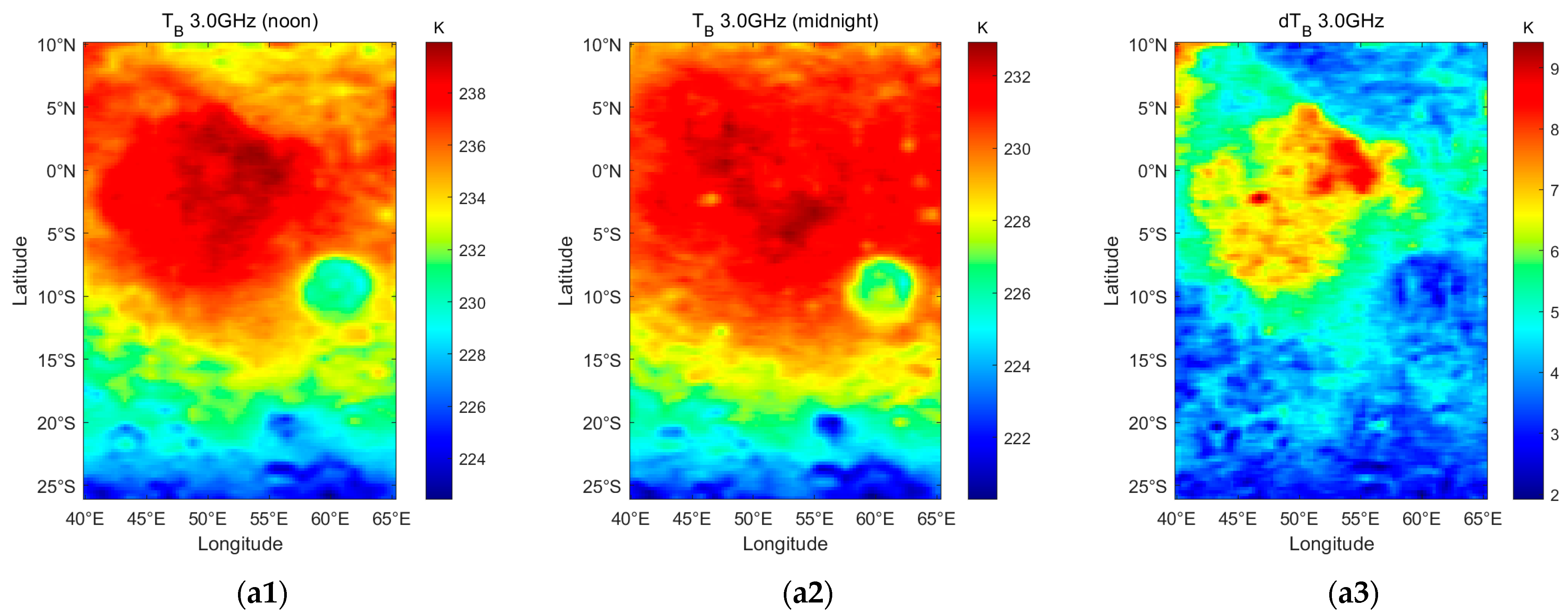
In this paper, we utilized the original CELMS data in the time spans from 13 to 14 o’clock as the noon brightness temperature TBnoon and 0 to 1 o’clock data as the midnight brightness temperature TBmidnight to generate brightness temperature maps. These time periods correspond to the highest and lowest temperatures on the lunar surface, respectively, and are therefore ideal for capturing the special microwave thermal emission (MTE) characteristics and thermophysical features of the basaltic units [23]. In addition, due to the limitation of the satellite orbit, only at this time can enough data points be obtained to support the study. The spatial resolution of CELMS data is 0.25° × 0.25°, about 7.5 × 7.5 km in Mare Fecunditatis. In our previous work, it was proposed that the difference between the noon and midnight brightness temperatures (written as dTB) has great potential for observing mare units [18,19,20,21,22,23]:
d T B = T B n o o n T B m i d n i g h t
where TBnoon and TBmidnight denote the noon and midnight brightness temperatures of the same frequency channel, respectively. The heatmaps of all brightness temperature features in Mare Fecunditatis are shown in Figure 2.
Kramer et al., divided Mare Fecunditatis into five units, according to the FTA (FeO + TiO2 abundance) [30]—Ihtm (a late(?) Imbrian, mid- to high-Ti, high-Fe mare basalt), Chtr (high-Ti spread), Iltm (an Imbrian-age, low-Ti, mid-Fe mare basalt), Im (an early(?) Imbrian-age, very low Ti, low-Fe mare basalt) and Cc (crater ejecta)—which is illustrated in Figure 3. Ihtm, Chtr, Iltm and Im can be considered as four phases of mare basalt. Cc is the ejecta of the craters, such as the Langrenus Crater and the Taruntius Crater, over the basalt units. Unlike other mare basins, Mare Fecunditatis is affected by a large crater—Langrenus. The ejecta of Langrenus spreads over the east part of Mare Fecunditatis and covers the mare basalt. In other words, this part combines crater ejecta and mare basalt.
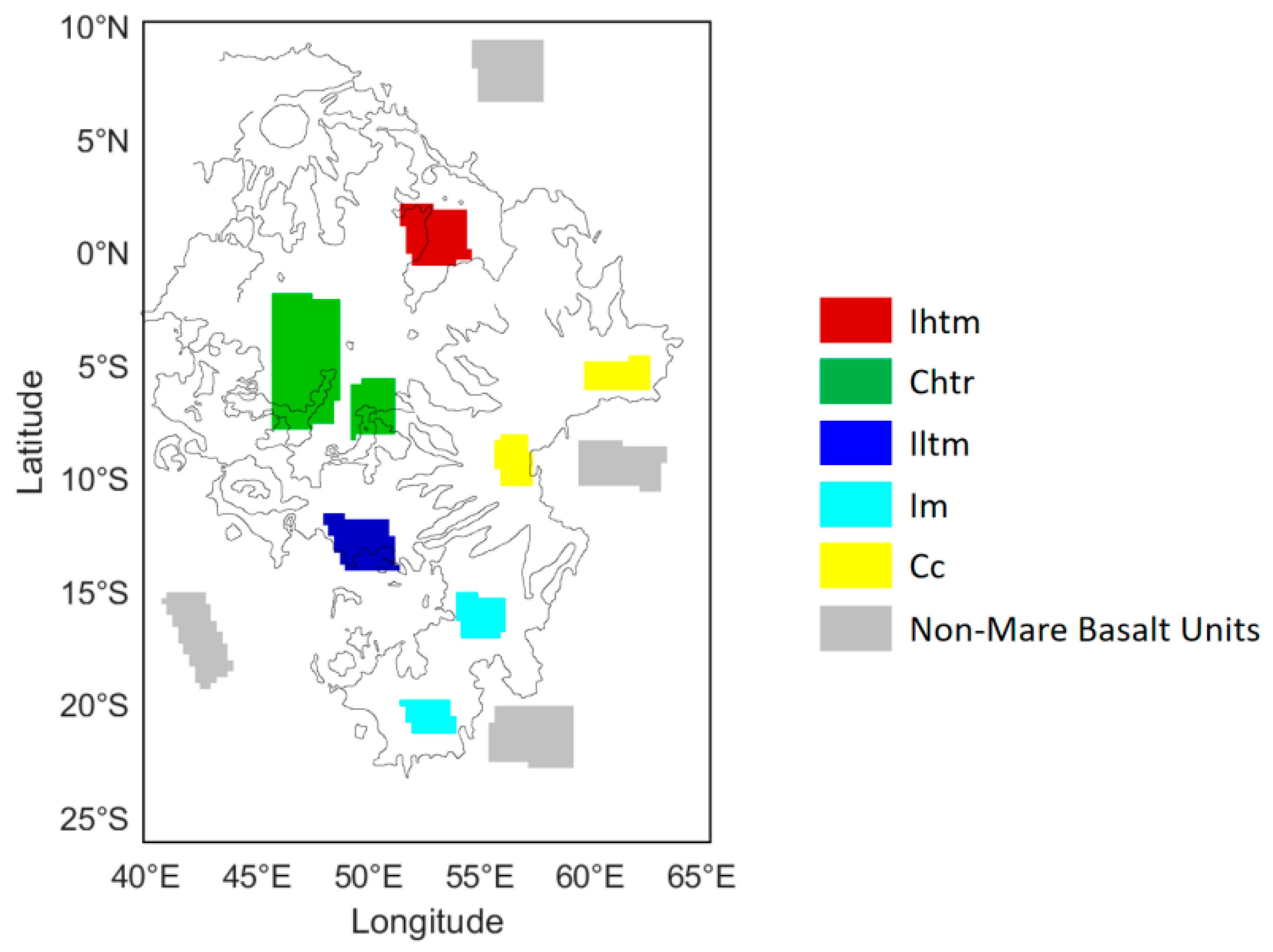
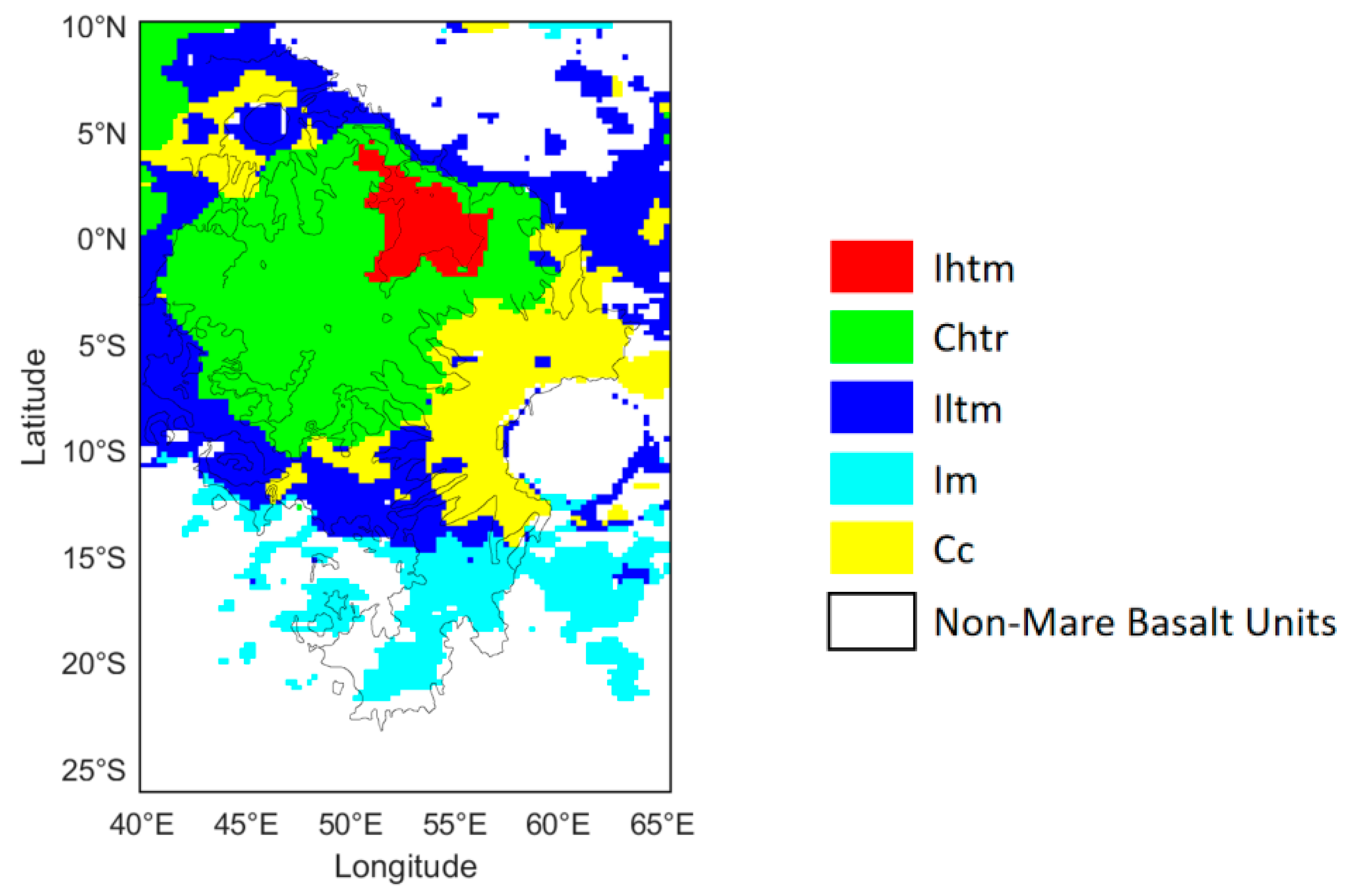
According to the class proposed by Kramer et al. [30], in this paper, we divided the basalt and ejecta units into five parts. As shown in Figure 4, the red, green, blue, cyan and yellow labels stand for the sample area of Ihtm, Chtr, Iltm, Im and Cc, respectively. The black line represents the boundary of geological units by Kramer et al. To map Mare Fecunditatis and its vicinity comprehensively in the following sections, we also labeled an individual class named “Non-Mare Basalt Units”, which includes non-basalt components, such as highland and Copernican craters.

3. Methodology

3.1. Overall Framework

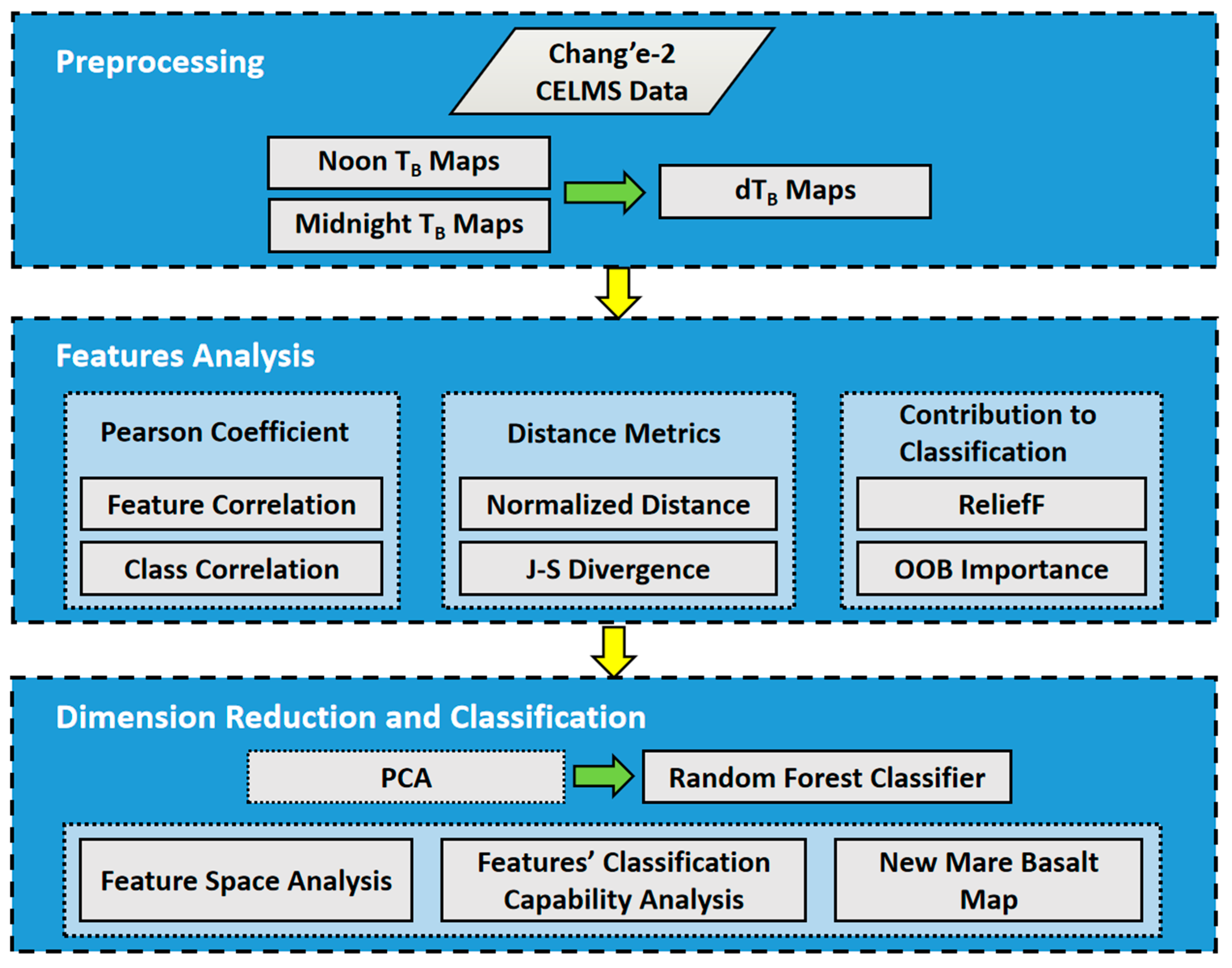
The overall framework of this paper is illustrated in Figure 5. The procedure include the following.
  • Preprocessing and brightness temperature feature exaction
The noon and midnight TB maps of Mare Fecunditatis with the frequencies of 3.0 GHz, 7.8 GHz, 19.35 GHz and 37.0 GHz are generated based on original CELMS data, and dTB maps are generated based on the difference between TBnoon and TBmidnight.
2.
Feature analysis
All brightness temperature features for distinguishing five mare geological units are evaluated in three aspects, including correlation analysis, distance metrics and contribution to classification. The Pearson coefficient is employed to assess feature redundancy and class linear separability. Normalized distance (ND) and J-S (Jensen–Shannon) divergence measure the Euclidean distance between two classes in the feature space and histogram separation, respectively. ReliefF and the out-of-bag (OOB) importance represent the contribution to classification for machine learning in different terms.
3.
Dimension reduction and classification
The random forest (RF) classifier is used to map Mare Fecunditatis. Principal component analysis (PCA) is conducted on 12 original features to reduce the dimension and analyze the feature space. A new geological map of Mare Fecunditatis is generated by CELMS data, based on the supervised machine learning method.

3.2. TB and dTB Feature Extraction

The TBnoon, TBmidnight and dTB features with different frequencies are generated based on CELMS data (12 features in total), which were introduced and displayed in Section 2.2.

3.3. Pearson Coefficient

In this study, we utilize the Pearson coefficient to quantify the level of correlation between each feature and the linear separability among classes.
The Pearson coefficient measures the degree of linear correlation, defined as the quotient of covariance and the standard deviation between two variables [31]:
ρ X , Y = C o v X , Y σ X σ Y
where Cov is the covariance between variables X and Y, and σ denotes the standard deviation. The Pearson coefficient ranges from −1 to 1, and its absolute value close to 1 reflects high correlation, and close to 0 means an uncorrelated relation.
From a feature engineering perspective, a high correlation coefficient typically indicates feature redundancy, while a low correlation coefficient suggests independent features. In terms of class-by-class correlation, a higher correlation coefficient indicates that the corresponding classes are more difficult to classify.

3.4. Distance Metrics

Two distance metrics, normalized distance [32] and J-S divergence [33], are considered to quantitatively evaluate the degree of separation among TB features. Typically, a higher degree of separation indicates better classification performance in machine learning.

3.4.1. Normalized Distance

Normalized distance is defined as:
d n o r m = μ 1 μ 2 σ 1 + σ 2
where μ and σ denote the mean and standard deviation of class 1 and class 2, respectively. Normalized distance measures the Euclidean distance between two classes without the influence of standard deviation, representing the separation of centers between different classes.

3.4.2. J-S Divergence

J-S divergence, an improved version of K-L divergence, indicates the separability of the two histograms. K-L divergence is also called relative entropy, which is defined as:
K L ( p | | q ) = p x l o g p x q x
where p and q represent the probability density of two classes. From Equation (3), it can be recognized that the order of p and q influences the result of the K-L divergence. J-S divergence solves this problem by using a symmetrical weighting operation:
J S ( p | | q ) = 1 2 K L ( p | | p + q 2 ) + 1 2 K L ( q | | p + q 2 )
The larger J-S divergence value means a higher degree of separation between two histograms or probability density distributions, as well as better classification capability. It has been proved that the J-S divergence value equals ln2 (approximately 0.6931) when two histograms are completely separated [34].

3.5. Contribution to Classification

To further understand the contribution and importance of brightness temperature features in the mare basalt classification process using machine learning methods, we employed two feature selection approaches—ReliefF and out-of-bag importance—to assess the contribution.

3.5.1. ReliefF

Relief (Relevant Features) is a filtering feature selection algorithm, in which a kind of weighting statistic method is designed before the features are inputted into the classifier [35]. Suppose a training set D:
D = x 1 , y 1 , x 2 , y 2 , ... , x m , y m
where x and y represent the training data and its label, m, denotes the number of train data. For each xi, the nearest samples xi,nh in the same class of xi are chosen and named “near-hit”, then the nearest samples xi,nm in the different class of xi are chosen and named “near-miss”, and the weight of the corresponding statistic is updated by:
δ j = i d i f f x i j x i , n h j 2 + d i f f x i j x i , n m j 2
where xaj is the value of sample xa in class j. For continuous data, diff() is defined as:
d i f f x a j , x b j = x a j x b j
From Equation (6), it can be observed that if the distance between xi,nm, and xi is larger than that between xi,nh, and xi, the whole weight will increase and the corresponding feature will benefit the classification. On the contrary, this feature does not contribute much to the classification process.
The Relief method was designed for binary classification. For multiclass classification, its variant ReliefF was proposed. Suppose the samples are from |υ| classes. ReliefF finds the nearest-hit of xi in class k as xi,nh, then finds the nearest-miss in each class, except class k, and is written as xi,l,nm (l = 1,2,…,|υ|; l ≠ k). The weight of ReliefF is updated as:
δ j = i d i f f x i j x i , n h j 2 + l k ( p l × d i f f x i j x i , n h j 2 )
where pl is the proportion of samples in class l.

3.5.2. OOB Importance

The OOB error is used for assessing the feature or variable importance in the Random Forest classifier [36,37]. It evaluates the change of classification performance by adding noise to features or variables. For a Random Forest classifier [38], not all data are input into each decision tree, but part of the data is randomly drawn. The remainder is called out-of-bag data. If a feature is added in stochastic noise that results in a decrease in accuracy, it can be considered that this feature is important for classification. The OOB importance of a decision tree is defined as the difference between OOB errors, with and without adding stochastic noise:
V = e r r 1 e r r 2
where err1 and err2 are out-of-bag errors with and without adding noise. Suppose there are N trees in the Random Forest, the OOB importance of this Random Forest is:
V I = 1 N i V i
The higher OOB importance value of a feature means that noise impacts more on the classification process, indicating this feature is more contributory, and vice versa [39]. The details of the Random Forest classifier will be introduced in Section 3.7.

3.6. Principal Component Analysis

Principal component analysis (PCA) is a dimension reduction method [35,40] via linearly projecting original data into low-dimension space, whose goal is to find a new feature space with the largest variance so that highly related features are compressed and effective ones can be enhanced.
Suppose the data Xn×p contains p variables and n samples, then the covariance matrix Σ is:
Σ p × p = X X T
And the eigenvalue matrix is calculated by:
Λ p × p = U T Σ U
where U = [u1, u2, ..., up] contains the eigenvectors of X. (12) can be detailed written as:
λ 1 λ 2 λ p = u 1 u 2 u p Σ u 1 u 2 u p
where λ1, λ2, ..., λp are eigenvalues of X. Note that eigenvalues correspond with eigenvectors. Then PCA data matrix is defined as:
Y = X U m = X u 1 u 2 u m
where 1 ≤ mp. m stands for top m principal components (PC). By this step, the data can be reduced to m dimensions [41]. The criterion of choosing m is:
i = 1 m λ i i = 1 p λ i t
Commonly, t can be set as 80% to 95% according to the situation.
PCA has been widely used in remote sensing image processing to extract effective information from multiple feature inputs [41,42,43]. For CELMS brightness temperature data, it consists of different frequencies and acquisition times, forming multiple features. So, introducing PCA is necessary to reduce the feature dimension in this study.

3.7. Random Forest

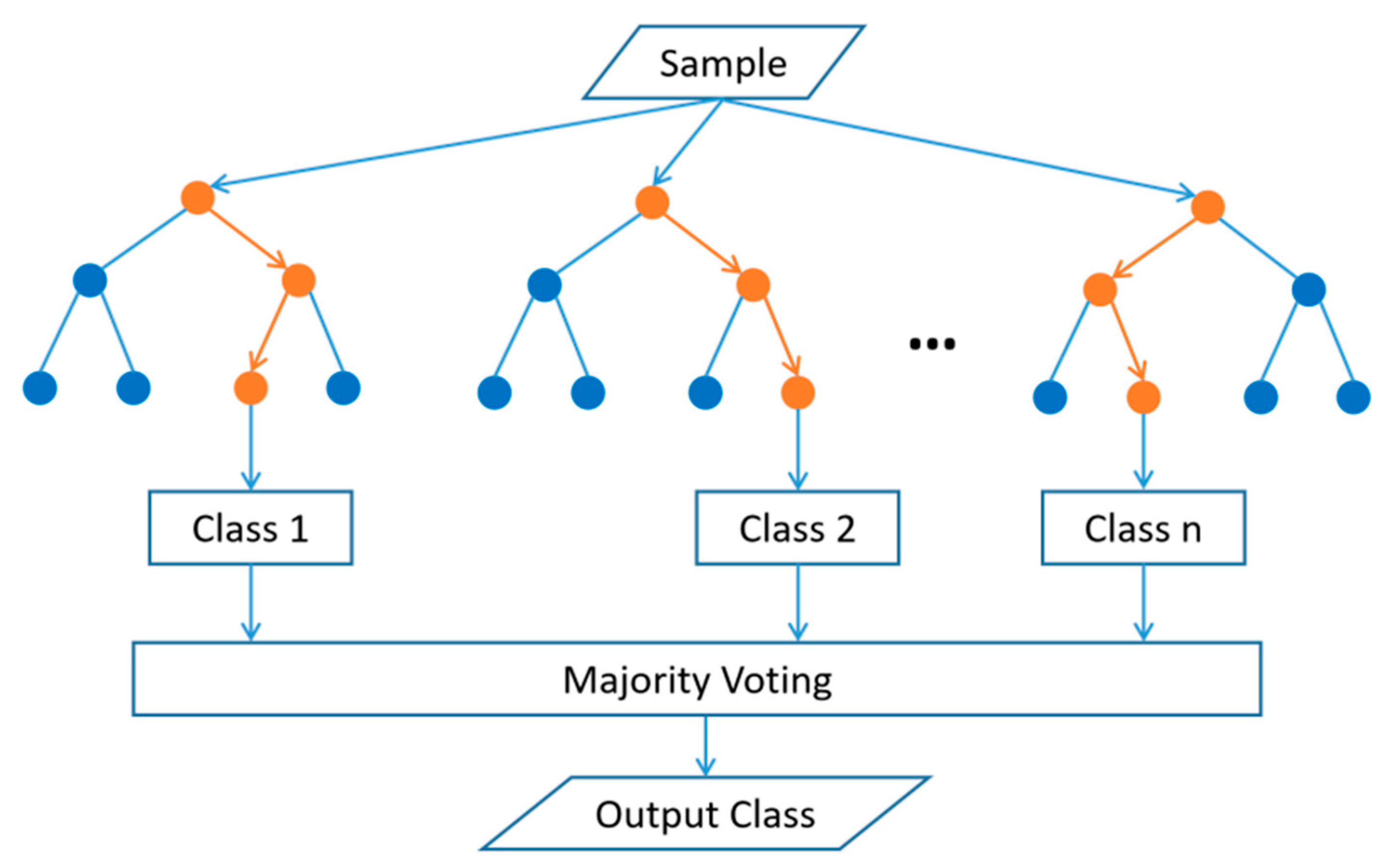
Random Forest (RF) is an ensemble learning method that integrates several decision trees to derive the classification result [38,44]. Each decision tree in a random forest is independently established and not related to each other. Once the forest is established, each input sample is judged separately and assigned to a class. Then, majority voting is used to combine all the outputs and predict the class of the input sample. The illustration of RF is shown in Figure 6.
Till now, the random forest classifier outperforms other ones in remote sensing image classification owing to its ensemble learning approach [33,45,46,47]. Consequently, we have chosen RF as the supervised classifier to automatically map Mare Fecunditatis in this study.

4. Experimental Results

4.1. Statistic Analysis

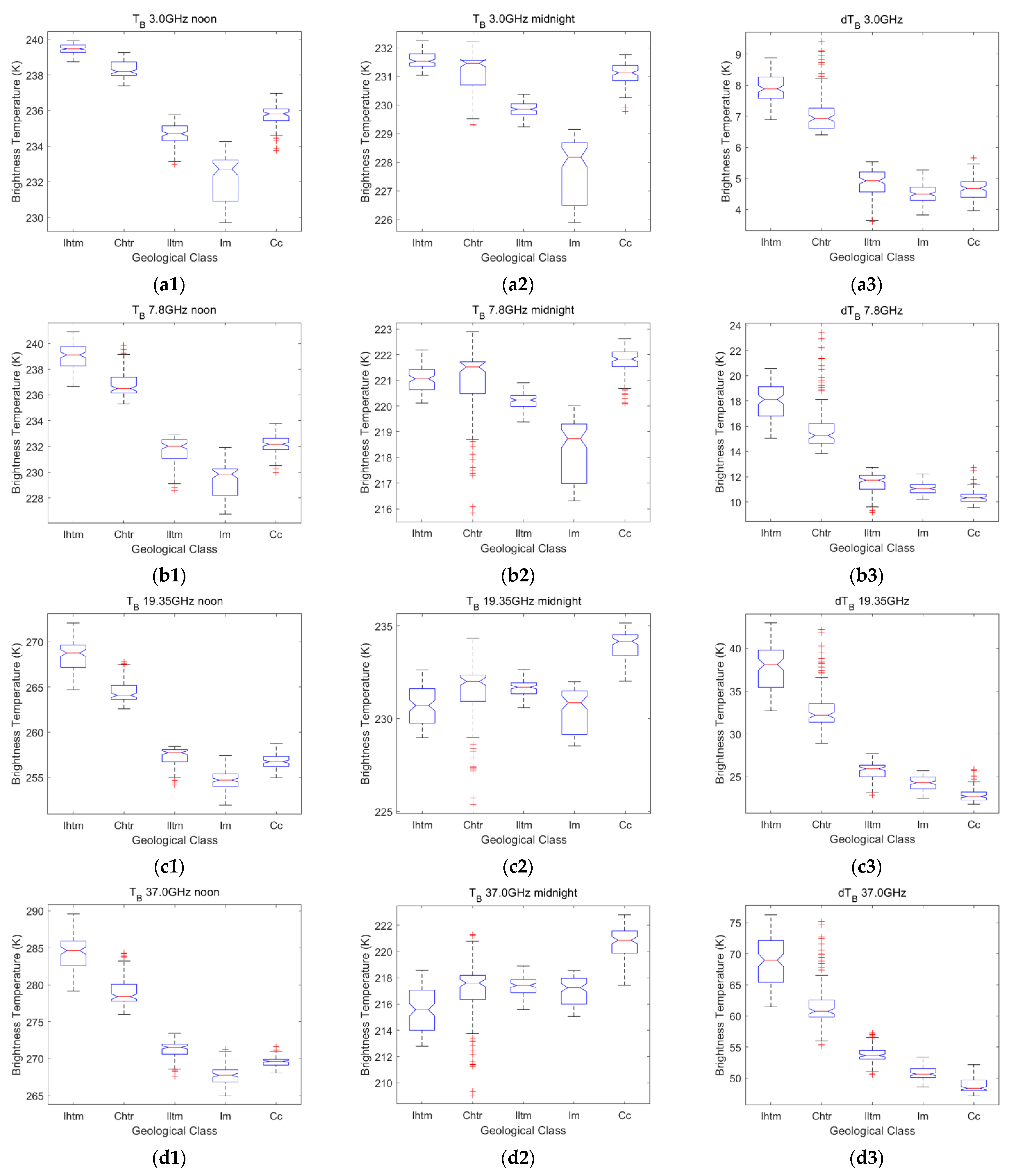
To understand the distribution of brightness temperatures for each basalt unit in different channels, the normalized histograms of each feature, also named the probability density function (PDF), are shown in Figure 7. In Figure 8, boxplots of the study samples in all features are demonstrated to further visualize and compare the difference in data distribution. From a general perspective, the classes {Ihtm, Chtr} vs. {Iltm, Im, Cc} can be easily distinguished in TBnoon features and dTB features. In TBmidnight features, all classes are confused, while Iltm, Im, Cc can be separated to some degree. Iltm, Im and Cc may be confused in TBnoon features and dTB features, and Ihtm and Chtr are confused in TBmidnight features.

4.2. Pearson Coefficient

We use the Pearson coefficient to calculate the feature correlation and class correlation.
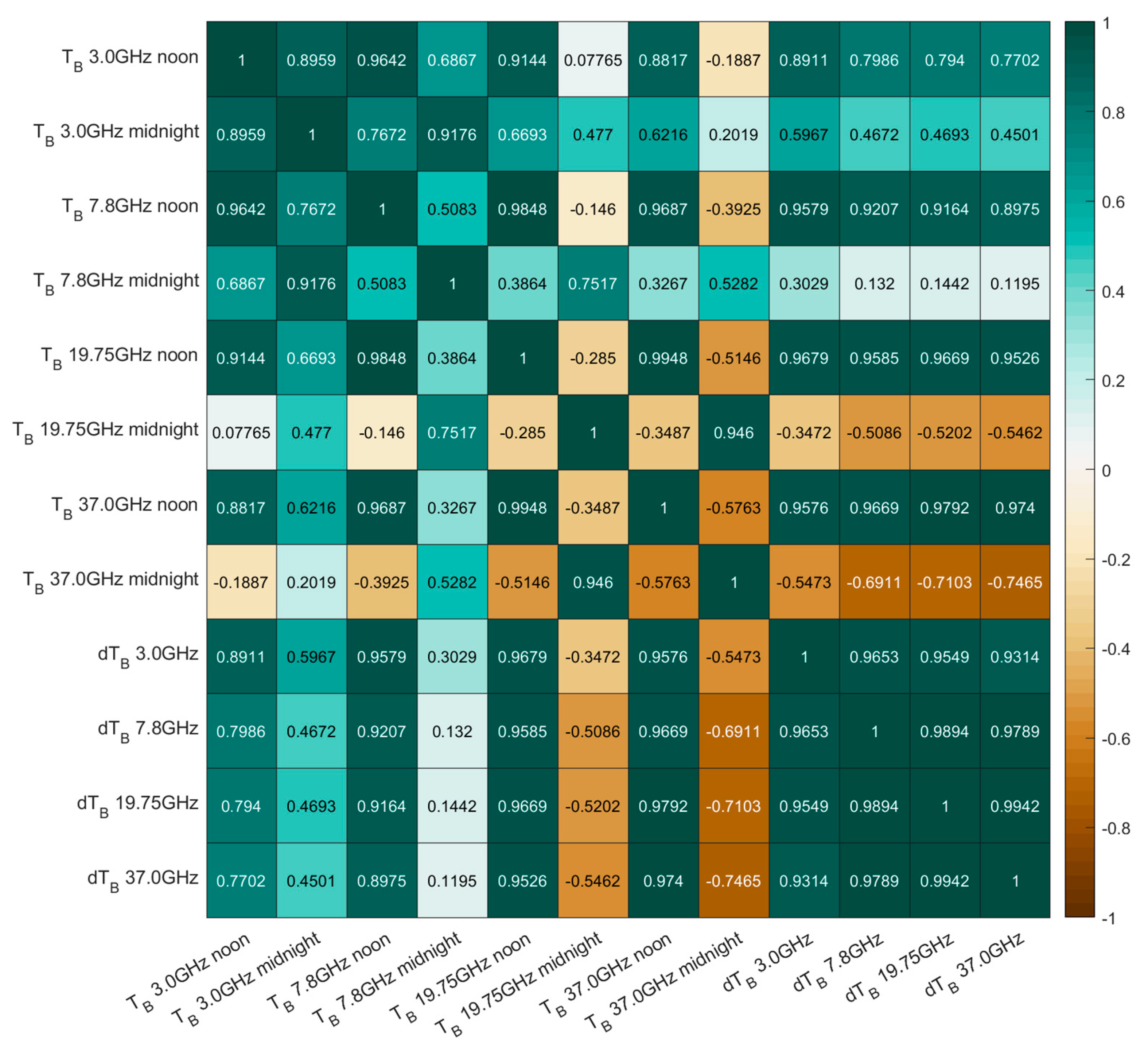
From the point of view of machine learning, a high correlation between two features (coefficient approximates 1 or −1) indicates redundancy, while a coefficient around zero suggests independence. To study the extent of feature redundancy, the feature-by-feature correlation is calculated, and the corresponding heatmap is generated in Figure 9, which reveals the relation among all the brightness temperature features.
Generally, dTB features have a high positive correlation. TBnoon features also have a high positive correlation, but it decreases as the frequency (corresponding with the penetration depth) increases. The correlation between dTB features and TBnoon features increases with the frequency. Particularly, all 19.35 GHz and 37.0 GHz TBnoon features have a high positive correlation with all dTB features. Features among TBmidnight and between TBmidnight and dTB show the tendency of transitioning from a positive correlation to uncorrelation and then to negative correlation. What is more, features with a closer frequency exhibit a higher correlation. Overall, a significant redundancy exists among these brightness temperature features.
The class-by-class correlation coefficient is also analyzed and shown in Figure 10. We found that an extremely high correlation exists among Iltm, Im and Cc, indicating that distinguishing these three basalt units in CELMS data would be challenging. In addition, the correlation decreases in the order of Ihtm → Chtr → Iltm → Im → Cc, which is highly consistent with the phase of the mare basalt eruption and formation.

4.3. Distance Metrics

Table 1 presents the normalized distance results calculated class by class. In general, TBnoon features tend to be appropriate for classifying the majority of basalt units, except for Iltm, Im and Cc. On the other hand, TBmidnight features are effective in distinguishing these three units (except high-frequency TBmidnight features for Im-Iltm). dTB features are generally not suitable for distinguishing basalt units among Iltm, Im, Cc and Ihtm-Chtr, while they are quite effective for other classes. Especially, dTB 37.0 GHz is suitable for distinguishing Cc-Iltm and Im-Iltm, and dTB 3.0 GHz is not quite adept at classifying Iltm-Cc and Cc-Im. Moreover, for all features, the normalized distance values between Ihtm and Chtr are all smaller than that between other classes, indicating that they are difficult to distinguish.
In Table 2, J-S divergence results are presented. Unlike normalized distance, J-S divergence measures the separability of the histogram. Note that the J-S divergence equal to 0.6931 means the histograms are completely separated [34], which was introduced in Section 3.4.2. For TBnoon features, their J-S divergence values are higher than TBmidnight features for most classes, which further demonstrated the effectiveness of TBnoon. For TBmidnight features, their separability of Cc-Im and Cc-Iltm performs significantly better than TBnoon and dTB features. dTB features show their unique superiority for distinguishing most of the basalt classes, except Cc, Im and Iltm. In addition, high-frequency dTB features are fit to classify Cc-Iltm and Im-Iltm.

4.4. Contribution to Classification

In this section, two feature selection methods—Relief(F) and OOB importance—are applied to quantitatively evaluate the features’ contribution to classification. Their principles are quite different: ReliefF is a filtering selection method, measuring the contribution based on the average Euclidean distance, while OOB importance is a wrapper selection method, indirectly assessing the feature importance by adding stochastic perturbation.
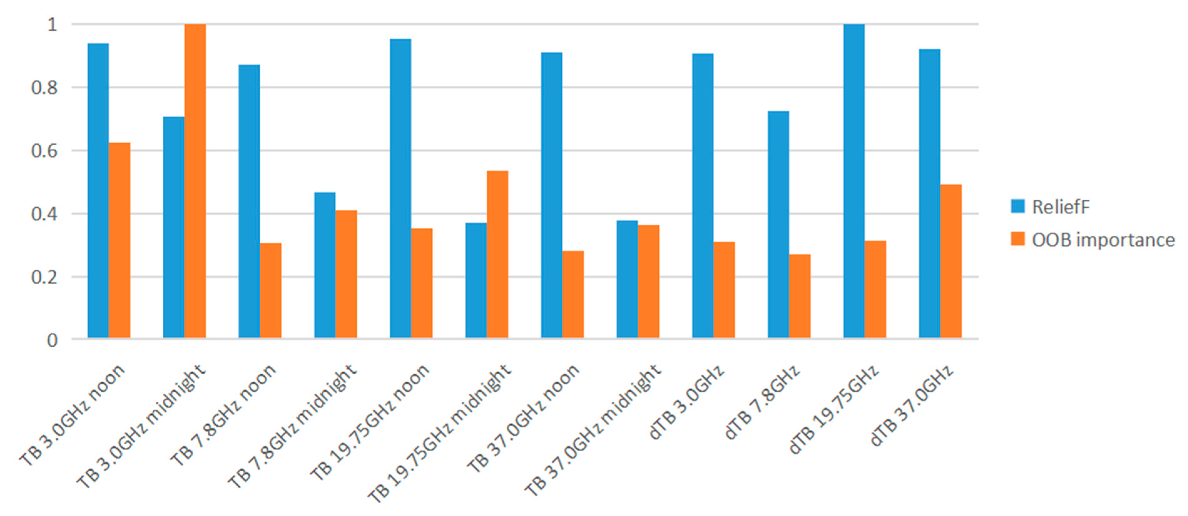
All brightness temperature features are assessed in two ways, namely, class-by-class and all-classes calculations. Table 3 and Table 4 present the class-by-class contribution, and all-classes contribution results are illustrated in Figure 11. The results of ReliefF largely agree with the conclusion in Section 4.3, which proves that TBnoon features are suitable for distinguishing classes of Ihtm-Chtr, Ihtm-Iltm, Ihtm-Cc, Ihtm-Im, Chtr-Cc, Chtr-Iltm and Chtr-Im compared with TBmidnight features, and TBmidnight features show their advantages in classifying Cc-Im, Cc-Iltm and Im-Iltm, while dTB features are appropriate for classifying most classes. Because the TBnoon features present the superiority of distinguishing more classes, their all-classes contribution weights for TBnoon features are higher than those for TBmidnight features. The 19.35 GHz and 37.0 GHz dTB features show their superiority for distinguishing Cc-Iltm, which also accords with the conclusion drawn in Section 4.3.
However, interestingly, the class-by-class OOB importance values of TBmidnight features are equal to 0 in most cases. Nonetheless, the all-classes OOB importance values (shown in Figure 11) of TBmidnight features are higher than those of TBnoon features. This phenomenon can be attributed to the superior ability of the TBmidnight features to distinguish Iltm, Im and Cc. In other words, other than distance metrics-based methods, such as ReliefF, OOB importance takes the “unique contribution” (a contribution that cannot be provided by any other features) into consideration to a larger degree. For the class pairs Ihtm-Iltm, Ihtm-Cc, Chtr-Cc and Chtr-Iltm assessed by OOB importance, the TBnoon features perform better than TBmidnight features, proving that TBnoon features have advantages over TBmidnight features in classifying these classes, while TBmidnight features are more suitable for distinguishing Cc-Im and Cc-Iltm. Especially, dTB 37.0 GHz performs best for distinguishing Cc-Iltm, and dTB 37.0 GHz contributes little to the classification of Cc-Im.
In summary, from a comprehensive perspective of Section 4.3 and Section 4.4, we can draw a conclusion that TBnoon features and dTB features are suitable for classifying Ihtm-Iltm, Ihtm-Cc, Ihtm-Im, Chtr-Cc, Chtr-Iltm and Chtr-Im, but distinguishing Iltm, Im and Cc mostly depends on TBmidnight features, and dTB features are unsuitable for distinguishing Cc-Im, especially at 3.0 GHz. Plus, Ihtm and Chtr units have similar components and structures, so they are not easy to separate in terms of most features. However, it should be noted that the 3.0 GHz TBnoon feature has a significant and unique advantage in distinguishing them.

4.5. Dimension Reduction and Classification

To map the basalt phase distribution in Mare Fecunditatis, the Random Forest classifier, which has been widely used for remote sensing image classification [33,45,46,47], is employed to map Mare Fecunditatis based on the above-mentioned Chang’e-2 brightness temperature features. The only hyper-parameter in RF is the number of trees, which is set as 125 empirically. The training set is the same as the study sample depicted in Figure 4.
We input all original brightness temperature features into a Random Forest classifier, and the result is presented in Figure 12, which is highly consistent with the geological map presented by Kramer et al. [30] shown in Figure 2. The boundary of geological units by Kramer et al. are marked by black lines. In our result, Ihtm, Chtr, Iltm, Im and Cc are colored red, green, blue, cyan and yellow, respectively. The Ihtm, Chtr, Iltm and Cc units mapped by us and Kramer et al. are quite similar, while the Im unit is different to some extent. The other difference is that in our mapping result, the Taruntius Crater is filled with Iltm basalt, which is out of discussion in the map by Kramer et al [30].
Generally, the basalt phase in Mare Fecunditatis exhibits a ring-shaped distribution. Ihtm is concentrated in the center, and Chtr and Iltm form the outer rings. Im distributes to the south of Mare Fecunditatis, while Cc surrounds the Langrenus Crater and the Taruntius Crater. This is completely in accordance with the volcanic eruption period and the igneous process [30].
In the above sections, it was demonstrated that both redundant and irrelevant information exists in TB and dTB features. To make full use of Chang’e-2 CELMS data, reduce computational complexity and avoid the “curse of dimensionality”, PCA, a classical dimension-reduction method, is considered before applying the RF classifier. We conducted the PCA algorithm on all 12 brightness temperature features. The data after PCA still have 12 dimensions. In Figure 13, the contribution rate of PCs, which is the variance of each PC (equivalent to the eigenvalue of the covariance matrix) that has been introduced in Equation (16), is shown by the blue bar. The cumulative contribution rate is shown in the orange line. The top 2 PCs hold a cumulative contribution of 99.08%, which demonstrates the strong redundancy that exists in the original features and explains the necessity of applying PCA. After the 3rd PC, the contribution rates drop, indicating the 3rd to 12th PCs hold so little effective information that their contribution is weak. Note that the variance of the 5th to 12th PCs is so low that they can be ignored, so we do not display them there.
To better interpret the results of PCA, we use biplots to express the PCA feature space, which consists of data scatter points and vector projection. The biplots of the top three PCs are shown in Figure 14. The 1st–2nd PCs plane (Figure 14a) is first visualized, where the main contribution is concentrated. The gray line indicates the feature vector projection in the PCA space, and the red, green, blue, cyan and yellow points stand for the data distribution of Ihtm, Chtr, Iltm, Im and Cc, respectively. The orientation and length of the vectors stand for the degree of relation between the original features and PCs. The projection length of the feature vectors on PCs is called the loading coefficient. Generally, the TBnoon and TBmidnight features point to the positive direction of the 1st PC and the negative direction of the 2nd PC, respectively. Hence, the TBnoon features are propitious to classifying {Ihtm, Chtr} vs. {Iltm, Im, Cc} groups, while TBmidnight features are fit to distinguish Im and Cc. Especially, 37.0 GHz TBnoon greatly impacts the first PC, but hardly influences the second PC, and 37.0 GHz TBmidnight impacts the second PC greatly, but hardly affects the first PC, demonstrating their strong ability on classification. These conclusions mutually verify the findings drawn in the previous sections.
The angle between vectors reflects the correlation. Features among dTB, TBnoon and TBmidnight have a strong correlation. Features between dTB and 19.75 GHz TBnoon, as well as dTB and 37.0 GHz TBnoon, are also highly correlated. Moreover, the lower the frequency, the stronger the correlation. These conclusions are all in accordance with the analysis by Pearson coefficient as mutual-validation results. Ihtm and Chtr have similar components and basalt phases, so part of their samples is confused, but most of them can be distinguished in the 1st and 2nd PCs. In Figure 14b, the second PC has a relatively poor capability for classification. It can only effectively separate Cc vs. {Ihtm, Chtr} and Iltm vs. {Ihtm, Chtr}. Im can be easily classified from other classes in the 3rd PC. In Figure 14c, it is obvious that the 3rd PC contributes quite weakly compared with the 1st PC: the distribution interval of data in the 3rd PC is quite limited, and the direction of the feature vector centralizes to the 1st PC.
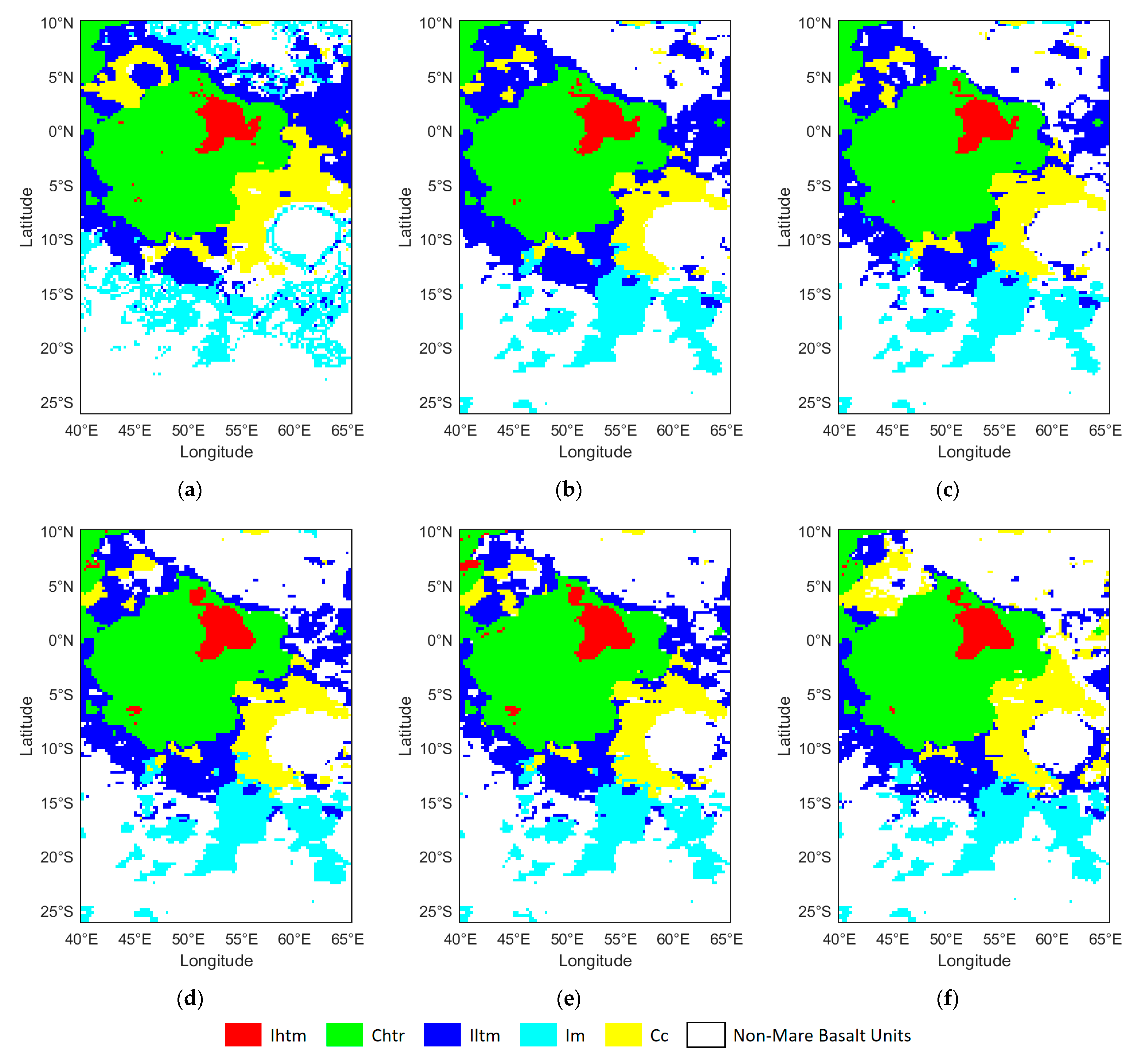
We classify the basalt units by jointly using PCA and RF. The top 2, 3, 4, 6, 8 and 12 PCs are selected for training the RF, and the classification results are shown in Figure 15. Obviously, in the classification result of the top two PCs, the effect of the Im unit is unsatisfactory, while the top three or four PCs produced good results, as the Im unit can be effectively separated from the other units, which verified the previous analysis. However, the results of the Taruntius Crater and its vicinity are largely different. The Taruntius Crater and its ejecta were classified as Iltm and Cc units, which is consistent with the original feature mapping result in the classification using the top two PCs. In other results, this area is misclassified or incompletely mapped to a certain degree. The mapping result of the Ihtm unit, Chtr unit and much of the Iltm unit are similar in the classification with all the PCA results. Moreover, the results of the top 6, 8 and 12 PCs make nearly no difference for their weak contribution.
Based on the above analysis, we suppose that the optimal choice of the number of dimensions in PCA is three, which is a good balance between low redundancy and high classification accuracy.
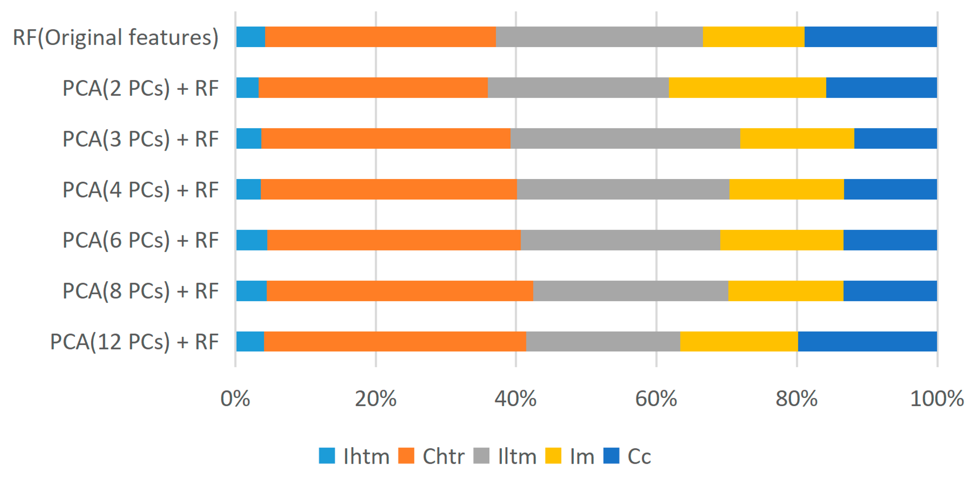
The proportions of geological units in Mare Fecunditatis and its vicinity mapped by each method are counted, and the corresponding bar charts are presented in Figure 16. Generally, the proportion of the geological units listed in descending order is Chtr, Iltm, Cc/Im, Ihtm.
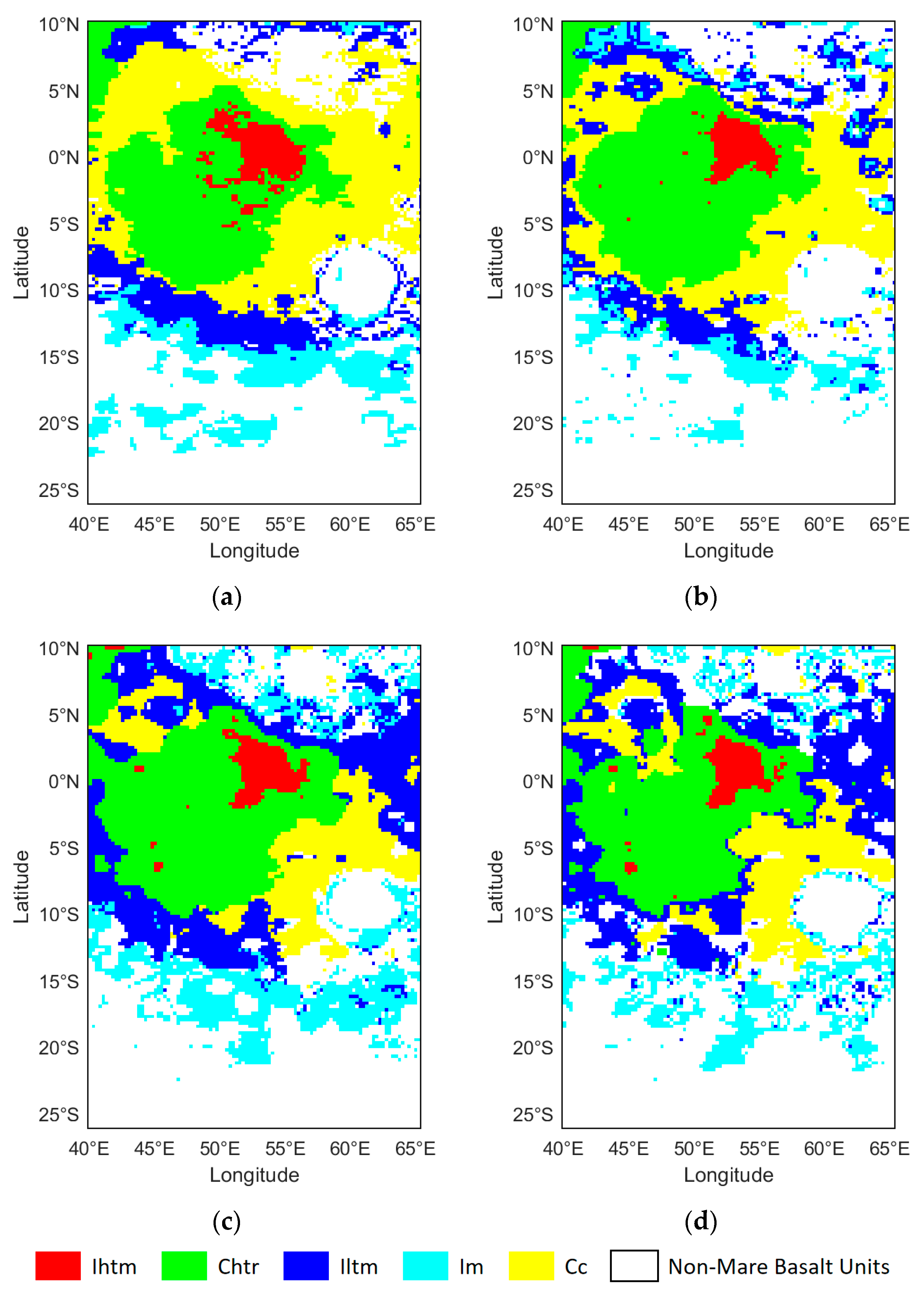
Ablation studies were designed and conducted to further understand the classification capability of each feature. Classification experiments were conducted by using 3.0 GHz features (3.0 GHz TBnoon, 3.0 GHz TBmidnight and dTB 3.0 GHz), 7.8 GHz features (7.8 GHz TBnoon, 7.8 GHz TBmidnight and dTB 7.8 GHz), 19.35 GHz features (19.35 GHz TBnoon, TB 19.35 GHz TBmidnight and dTB 19.35 GHz) and 37.0 GHz features (37.0 GHz TBnoon, 37.0 GHz TBmidnight and dTB 37.0 GHz), respectively, as shown in Figure 17. The results showed that the 3.0 GHz and 7.8 GHz features misclassified a certain extent of Chtr and Iltm units as Cc. The Taruntius Crater was almost entirely misclassified by the 3.0 GHz features group. In contrast, the 19.35 GHz features and 37.0 GHz features outperformed the lower frequency bands. Interestingly, the feature evaluation indices did not reveal significant contribution differences in frequency, but in this experiment, the high-frequency features yielded the best classification results.
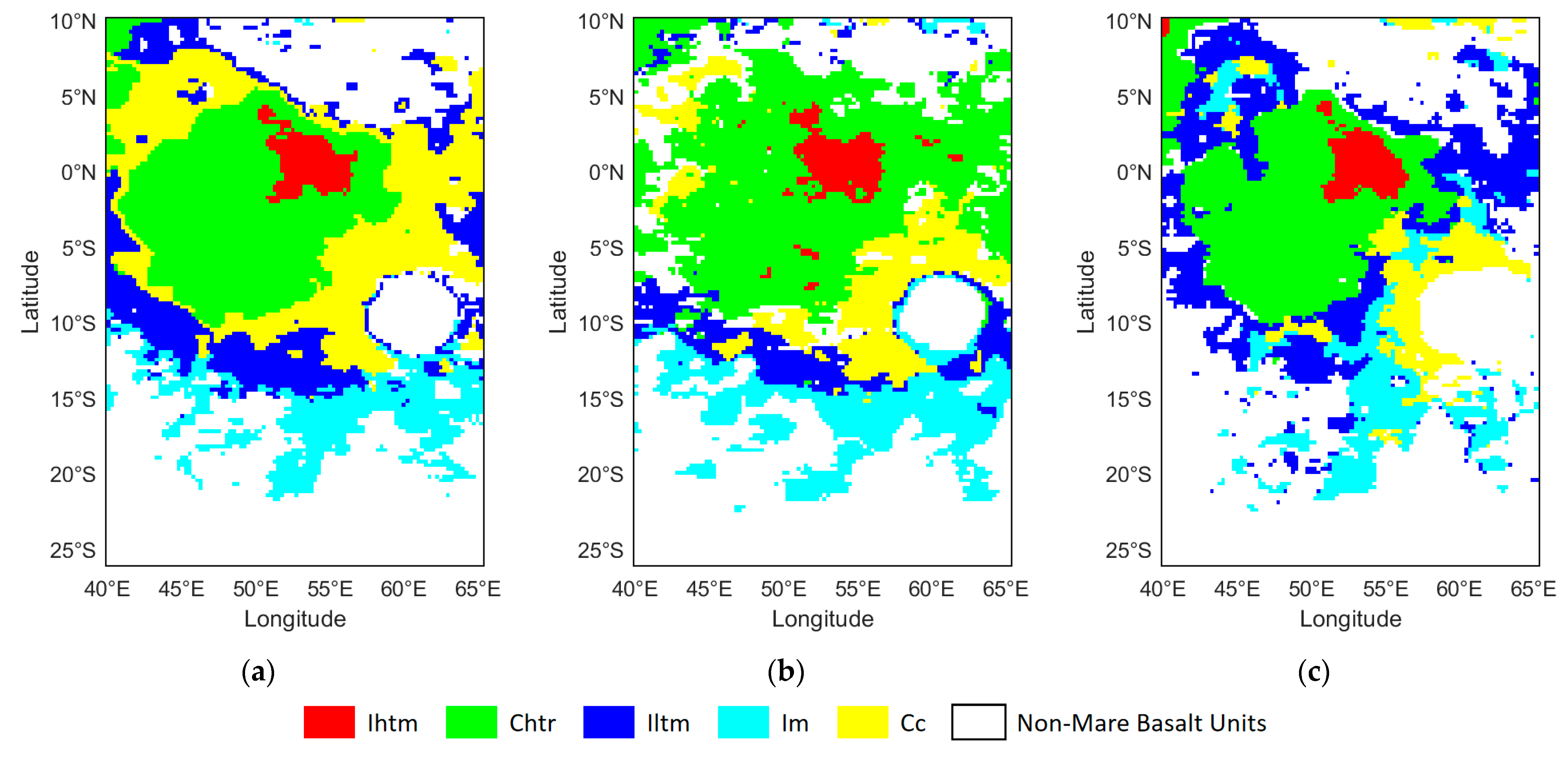
We also used the combination of TBnoon features, TBmidnight features and dTB features to map Mare Fecunditatis, and the results are shown in Figure 18. For TBnoon features, their result confuses Cc and Iltm largely. The mapping result of TBmidnight features appears chaotic, with a large-scale misclassification of the Chtr unit. Yet, the Cc and Im units are well-classified, which confirms the conclusions drawn in Section 4.3 and Section 4.4 For dTB features, the Im and Cc units are confused to some degree. Overall, our analysis demonstrates that each feature has its unique strengths and limitations in mapping mare units.

5. Discussions

In this paper, a unified framework of assessing CELMS data for mapping mare basalt units is proposed, followed by a case study on Mare Fecunditatis. To the best of our knowledge, this is the first study that systematically analyzes the brightness temperature features of Chang’e-2 CELMS data for each mare basin unit. Based on the experimental results, some conclusions can be drawn:
1.
TBnoon and TBmidnight features demonstrate different capabilities in distinguishing various basalt units. TBnoon features are good at distinguishing most class pairs, except those involving Cc, Im and Iltm, compared with TBmidnight features, while TBmidnight features showed their superiority in distinguishing Cc-Im and Cc-Iltm from TBnoon features. The possible explanation is that the different Ti and Fe content lead to varying cooling rates during the lunar night.
2.
The frequency range of the observation influences the capabilities in distinguishing different basalt units. High-frequency features with a shallow penetration depth, especially 19.35 GHz, can better map Mare Fecunditatis with fewer classification errors in Cc, Im and Iltm units. The possible explanation is that Im and Iltm are early-age(?) mare basalt, and together with the crater ejecta Cc, contain less Ti and are highly dielectric. Yet, 37.0 GHz features may be influenced by the lunar dust from the regolith, leading to a slightly poorer result. Low-frequency features (especially 3.0 GHz) may classify certain parts of mare basalt as Cc units. We suppose that the possible reason is that the deep layer of Mare Fecunditatis is the impact basin (interpreted as Cc unit) and was not filled by magma when the Mare Fecunditatis was formed (may be in the Imbrian period 3.2~3.85 Ga before) [27].
3.
The advantage of utilizing the dTB features proposed in our previous researches [18,19,20,21,22,23] in distinguishing most classes in CELMS data is confirmed in this study. dTB features are verified for their strong ability to eliminate the latitude difference and strengthen the difference of cooling effects of various basalt units. We also discovered that dTB features have a stronger ability to distinguish mare basalt, especially between early(?)- and late(?)-aged basalt, in certain aspects.
4.
Redundancy exists universally in CELMS features. This study points out the need to conduct dimension reduction on CELMS features. We discovered that only 3 PCs in the PCA feature space can represent almost all 12 original features for the first time. After dimension reduction, the difficult-to-identify Im unit hidden in the south part of Mare Fecunditatis is better classified. The scatterplots in PCA support this phenomenon.
5.
A new geological map of Mare Fecunditatis is generated in this study based on CELMS data by using the supervised machine learning method, which largely agreed with the previous mapping results by other researchers based on Clementine UV/VIS data [30,48,49,50], proving that CELMS data are effective in mapping mare basalt units.

6. Conclusions

In this paper, a framework is proposed to systematically assess the brightness temperature features of Chang’e-2 CELMS in Mare Fecunditatis. As far as we know, this is the first time Chang’e-2 CELMS TB data have been systematically analyzed, and based on this, a new geological map of Mare Fecunditatis was generated by using machine learning techniques. The basalt map derived from CELMS data demonstrates many similarities with the previous geological map provided by Kramer et al., while providing some new hints for understanding the vertical structure of the lunar surface regolith.
This study quantitatively analyzed the effect of each brightness temperature feature in mapping the mare basin from various perspectives. In future studies, an analysis will be conducted on more lunar regions of research interest, including the landing site of Chang’e-5, where the surface regolith ground truth is obtained by in situ measurements and returned sample analysis [51].
Furthermore, machine learning methods have proved their great feasibility for CELMS data. However, up to now, studies on CELMS data still mainly relied on manual interpretation. Recently, machine learning models have been gradually introduced into lunar and planetary research [52,53,54]. Further studies will explore the potential of more advanced machine learning models with regard to lunar brightness temperature analysis [55,56,57].
Additionally, fusing optical (such as WAC images and Clementine UV/VIS data) and microwave remote sensing for mapping the mare basin could be beneficial, as many studies on planetary surfaces mapping have proven that multisource remote sensing is helpful for improving classification accuracy [33,53,58,59,60,61].

Author Contributions

Conceptualization, Y.L., Z.M. and Y.Z.; methodology, Y.L. and Z.Y.; software, Z.Y.; validation, Y.L. and Z.Y.; formal analysis, Z.Y.; investigation, Z.Y. and Z.M.; resources, Y.L., Z.M., J.P. and Y.Z.; data curation, Z.M.; writing—original draft preparation, Y.L. and Z.Y.; writing—review and editing, Y.L. and Z.M.; visualization, Z.Y. and Z.M.; supervision, J.P. and Y.Z.; project administration, J.P.; funding acquisition, J.P. and Y.Z. All authors have read and agreed to the published version of the manuscript.

Funding

This work was supported in part by the National Key Research and Development Program of China (2021YFA0715101), the Strategic Priority Program of the Chinese Academy of Sciences (XDB41020104) and the Natural Science Foundation of China (41706201).

Data Availability Statement

The CELMS data were downloaded from the Lunar and Planetary Data Release System (https://moon.bao.ac.cn, accessed on 30 March 2022). The WAC images were obtained from the Quickmap website (https://quickmap.lroc.asu.edu, accessed on 13 October 2022) and by JMARS software (https://jmars.mars.asu.edu, accessed on 13 October 2022).

Acknowledgments

The CELMS data provided by the Lunar and Planetary Data Release System and the WAC images provided by the Quickmap website and JMARS software are highly appreciated. The authors sincerely thank Liu Jingwen and Liu Jianzhong from the Institute of Geochemistry, Chinese Academy of Sciences, for their valuable suggestions on this work.

Conflicts of Interest

The authors declare no conflict of interest.

References

  1. Tang, T.; Meng, Z.; Lian, Y.; Xiao, Z.; Ping, J.; Cai, Z.; Zhang, X.; Dong, X.; Zhang, Y. New Insights into Surface Deposits in the Balmer-Kapteyn Cryptomare Region Provided by Chang’E-2 Microwave Radiometer Data. Remote Sens. 2022, 14, 4556. [Google Scholar] [CrossRef]
  2. Meng, Z.; Tang, T.; Dong, X.; Chang, W.; Zou, M.; Zhang, H.; Wang, M.; Cai, Z.; Ping, J.; Zheng, Y.; et al. Analyzing the Microwave Thermal Emission Features of Lunar Regolith in Chang’E Landing Sites and Its Geologic Significance. Sci. Sin. Phys. Mech. Astron. 2022, 53, 239609. [Google Scholar] [CrossRef]
  3. Li, C.; Guo, Z.; Li, Y.; Tai, K.; Wei, K.; Li, X.; Liu, J.; Ma, W. Impact-driven disproportionation origin of nanophase iron particles in Chang’e-5 lunar soil sample. Nat. Astron. 2022, 6, 1156–1162. [Google Scholar] [CrossRef]
  4. Karthi, A.; Arivazhagan, S. Chronological and compositional mapping of the Mare Orientale basin using Chandrayaan-1–M3 and LRO datasets. Icarus 2022, 375, 114844. [Google Scholar] [CrossRef]
  5. Kramer, G.Y.; Jolliff, B.L.; Neal, C.R. Distinguishing high-alumina mare basalts using Clementine UVVIS and Lunar Prospector GRS data: Mare Moscoviense and Mare Nectaris. J. Geophys. Res. Planets 2008, 113, E01002. [Google Scholar] [CrossRef]
  6. Thiessen, F.; Besse, S.; Staid, M.I.; Hiesinger, H. Mapping lunar mare basalt units in mare Imbrium as observed with the Moon Mineralogy Mapper (M3). Planet. Space Sci. 2014, 104, 244–252. [Google Scholar] [CrossRef]
  7. Hiesinger, H.; Head, J.W., III; Wolf, U.; Jaumann, R.; Neukum, G. Ages and stratigraphy of lunar mare basalts in Mare Frigoris and other nearside maria based on crater size-frequency distribution measurements. J. Geophys. Res. Planets 2010, 115, E03003. [Google Scholar] [CrossRef] [Green Version]
  8. Liu, J.; Liu, J.; Wang, J.; Zhu, K.; Zhang, L. Basalt Chronology of the Orientale Basin Based on CE-2 CCD Imaging and Implications for Lunar Basin Volcanism. Remote Sens. 2022, 14, 1426. [Google Scholar] [CrossRef]
  9. Bugiolacchi, R.; Mall, U.; Bhatt, M.; McKenna-Lawlor, S.; Ullaland, K. From the Imbrium Basin to crater Tycho: The first regional spectral distribution map derived from SIR-2 near-infrared data. Icarus 2013, 223, 804–818. [Google Scholar] [CrossRef]
  10. Bugiolacchi, R.; Mall, U.; Bhatt, M.; McKenna-Lawlor, S.; Banaszkiewicz, M.; Brønstad, K.; Nathues, A.; Søraas, F.; Ullaland, K.; Pedersen, R.B. An in-depth look at the lunar crater Copernicus: Exposed mineralogy by high-resolution near-infrared spectroscopy. Icarus 2011, 213, 43–63. [Google Scholar] [CrossRef] [Green Version]
  11. Bugiolacchi, R.; Guest, J.E. Compositional and temporal investigation of exposed lunar basalts in the Mare Imbrium region. Icarus 2008, 197, 1–18. [Google Scholar] [CrossRef]
  12. Cao, H.; Xu, Y.; Xu, L.; Zhang, L.; Bugiolacchi, R.; Zhang, F. From Schrödinger to Von Kármán: An Intriguing New Geological Structure Revealed by the Chang’e-4 Lunar Penetrating Radar. Geophys. Res. Lett. 2023, 50, e2022GL101413. [Google Scholar] [CrossRef]
  13. Wang, P.; Bugiolacchi, R.; Su, Y. A new compositional, mineralogical and chronological study of the Leibnitz crater within the SPA basin. Planet. Space Sci. 2023, 227, 105640. [Google Scholar] [CrossRef]
  14. Chen, R.; Xu, Y.; Xie, M.; Zhang, L.; Niu, S.; Bugiolacchi, R. Sub-surface stratification and dielectric permittivity distribution at the Chang’E-4 landing site revealed by the lunar penetrating radar. Astron. Astrophys. 2022, 664, A35. [Google Scholar] [CrossRef]
  15. Zhang, L.; Xu, Y.; Bugiolacchi, R.; Hu, B.; Liu, C.; Lai, J.; Zeng, Z.; Huo, Z. Rock abundance and evolution of the shallow stratum on Chang’e-4 landing site unveiled by lunar penetrating radar data. Earth Planet. Sci. Lett. 2021, 564, 116912. [Google Scholar] [CrossRef]
  16. Cai, Z.; Lan, T. Lunar brightness temperature model based on the microwave radiometer data of Chang’E-2. IEEE Trans. Geosci. Remote Sens. 2017, 55, 5944–5955. [Google Scholar] [CrossRef]
  17. Jin, Y.; Fa, W. Theoretical Methods and Applications of Planetary Microwave Remote Sensing; Science Press: Beijing, China, 2019. [Google Scholar]
  18. Meng, Z.G.; Wang, H.H.; Zheng, Y.C.; Wang, Y.Z.; Miyamoto, H.; Cai, Z.C.; Zhu, Y.Z. Several Geological Issues of Schrödinger Basin Exposed by CE-2 CELMS Data. Adv. Astron. 2019, 2019, 3926082. [Google Scholar] [CrossRef]
  19. Meng, Z.; Li, X.; Chen, S.; Zheng, Y.; Shi, J.; Wang, T.; Zhang, Y.; Ping, J.; Lu, Y. Thermophysical features of shallow lunar crust demonstrated by typical copernican craters using CE-2 CELMS data. IEEE J. Sel. Top. Appl. Earth Obs. Remote Sens. 2019, 12, 2565–2574. [Google Scholar] [CrossRef]
  20. Hu, S.; Meng, Z.; Zhu, Y.; Lian, Y.; Li, C.; Guesv, A. Microwave Emission Features of Von Kármán Crater Revealed by Chang’E-2 CELMS Data. J. Deep. Space Explor. 2018, 5, 20–26. [Google Scholar] [CrossRef]
  21. Meng, Z.; Zhao, R.; Cai, Z.; Ping, J.; Tang, Z.; Chen, S. Microwave thermal emission at Tycho area and its geological significance. IEEE J. Sel. Top. Appl. Earth Obs. Remote Sens. 2022, 10, 2984–2990. [Google Scholar] [CrossRef]
  22. Lei, J.; Meng, Z.; Wang, Y.; Huang, S.; Ping, J.; Cai, Z.; Zhang, Y. Potential Applications of CE-2 Microwave Radiometer Data in Understanding Basaltic Volcanism in Heavily Ejecta-Contaminated Mare Frigoris. Remote Sens. 2022, 14, 2725. [Google Scholar] [CrossRef]
  23. Meng, Z.; Chen, S.; Wang, Y.; Wang, T.; Cai, Z.; Zhang, Y.; Zheng, Y.; Hu, S. Reevaluating Mare Moscoviense and its vicinity using Chang’E-2 microwave sounder data. Remote Sens. 2020, 12, 535. [Google Scholar] [CrossRef] [Green Version]
  24. Li, Y.; Zhang, Y.; Yuan, Z.; Guo, H.; Pan, H.; Guo, J. Marine oil spill detection based on the comprehensive use of polarimetric SAR data. Sustainability 2018, 10, 4408. [Google Scholar] [CrossRef] [Green Version]
  25. Mazhar, S.; Sun, G.; Bilal, A.; Hassan, B.; Li, Y.; Zhang, J.; Lin, Y.; Khan, A.; Ahmed, R.; Hassan, T. AUnet: A Deep Learning Framework for Surface Water Channel Mapping Using Large-Coverage Remote Sensing Images and Sparse Scribble Annotations from OSM Data. Remote Sens. 2022, 14, 3283. [Google Scholar] [CrossRef]
  26. Li, Y.; Yang, J.; Yuan, Z.; Zhang, Y. Marine Oil Spills Detection and Classification from PolSAR Images Based on Complex-Valued Convolutional Neural Network. In Proceedings of the 2022 IEEE International Geoscience and Remote Sensing Symposium, Kuala Lumpur, Malaysia, 17–22 July 2022. [Google Scholar] [CrossRef]
  27. Zhao, S.; Qian, Y.; Xiao, L.; Zhao, J.; He, Q.; Huang, J.; Wang, J.; Chen, H.; Xu, W. Lunar Mare Fecunditatis: A Science-Rich Region and a Concept Mission for Long-Distance Exploration. Remote Sens. 2022, 14, 1062. [Google Scholar] [CrossRef]
  28. Ouyang, Z. Introduction to Lunar Science; China Astronautic Publishing House: Beijing, China, 2005. [Google Scholar]
  29. Fortezzo, C.M.; Spudis, P.D.; Harrel, S.L. Release of the digital unified global geologic map of the Moon at 1: 5,000,000-Scale. In Proceedings of the Lunar and Planetary Science Conference, Woodlands, TX, USA, 6–20 March 2020; Available online: https://www.hou.usra.edu/meetings/lpsc2020/pdf/2760.pdf (accessed on 29 March 2023).
  30. Kramer, G.Y.; Jolliff, B.L.; Neal, C.R. Searching for high alumina mare basalts using Clementine UVVIS and Lunar Prospector GRS data: Mare Fecunditatis and Mare Imbrium. Icarus 2008, 198, 7–18. [Google Scholar] [CrossRef]
  31. Li, Y.; Liang, H.; Sun, G.; Yuan, Z.; Zhang, Y.; Zhang, H. A Land Cover Background-Adaptive Framework for Large-Scale Road Extraction. Remote Sens. 2022, 14, 5114. [Google Scholar] [CrossRef]
  32. Li, Y.; Lin, H.; Zhang, Y.; Chen, J. Comparisons of circular transmit and linear receive compact polarimetric SAR features for oil slicks discrimination. J. Sens. 2015, 2015, 631561. [Google Scholar] [CrossRef] [Green Version]
  33. Bai, Y.; Sun, G.; Li, Y.; Ma, P.; Li, G.; Zhang, Y. Comprehensively analyzing optical and polarimetric SAR features for land-use/land-cover classification and urban vegetation extraction in highly-dense urban area. Int. J. Appl. Earth Obs. Geoinf. 2021, 103, 102496. [Google Scholar] [CrossRef]
  34. Farnia, F.; Tse, D. A convex duality framework for GANs. In Proceedings of the 32nd Conference on Neural Information Processing Systems, Montreal, QC, Canada, 2–8 December 2018; Available online: https://proceedings.neurips.cc/paper/2018/file/831caa1b600f852b7844499430ecac17-Paper.pdf (accessed on 27 October 2022).
  35. Zhou, Z. Machine Learning; Tsinghua University Press: Beijing, China, 2018. [Google Scholar]
  36. Genuer, R.; Poggi, J.M.; Tuleau-Malot, C. Variable selection using random forests. Pattern Recognit. Lett. 2010, 31, 2225–2236. [Google Scholar] [CrossRef] [Green Version]
  37. Breiman, L. Out-of-Bag Estimation. 1996. Available online: https://www.stat.berkeley.edu/~breiman/OOBestimation.pdf (accessed on 27 October 2022).
  38. Breiman, L. Random forests. Mach. Learn. 2001, 45, 5–32. [Google Scholar] [CrossRef] [Green Version]
  39. Gao, S.; Li, S.; Liu, H. Oil Spill Detection by CP SAR Based on the Power Entropy Decomposition. Remote Sens. 2022, 14, 5030. [Google Scholar] [CrossRef]
  40. Fu, H.; Sun, G.; Ren, J.; Zhang, A.; Jia, X. Fusion of PCA and segmented-PCA domain multiscale 2-D-SSA for effective spectral-spatial feature extraction and data classification in hyperspectral imagery. IEEE Trans. Geosci. Remote Sens. 2020, 60, 1–14. [Google Scholar] [CrossRef]
  41. Zhang, T.; Marino, A.; Xiong, H.; Yu, W. A ship detector applying principal component analysis to the polarimetric notch filter. Remote Sens. 2018, 10, 948. [Google Scholar] [CrossRef] [Green Version]
  42. Zhang, Y.; Li, Y.; Liang, X.S.; Tsou, J. Comparison of oil spill classifications using fully and compact polarimetric SAR images. Appl. Sci. 2017, 7, 193. [Google Scholar] [CrossRef] [Green Version]
  43. Chen, G.; Li, Y.; Sun, G.; Zhang, Y. Application of deep networks to oil spill detection using polarimetric synthetic aperture radar images. Appl. Sci. 2017, 7, 968. [Google Scholar] [CrossRef]
  44. Zhang, C.; Ma, Y. Ensemble Machine Learning: Methods and Applications; Springer Science & Business Media: New York, NY, USA, 2012. [Google Scholar] [CrossRef]
  45. Belgiu, M.; Drăguţ, L. Random forest in remote sensing: A review of applications and future directions. ISPRS J. Photogramm. Remote Sens. 2016, 114, 24–31. [Google Scholar] [CrossRef]
  46. Zhang, H.; Li, J.; Wang, T.; Lin, H.; Zheng, Z.; Li, Y.; Lu, Y. A manifold learning approach to urban land cover classification with optical and radar data. Landsc. Urban Plan. 2018, 172, 11–24. [Google Scholar] [CrossRef]
  47. Zhang, H.; Lin, H.; Wang, Y. A new scheme for urban impervious surface classification from SAR images. ISPRS J. Photogramm. Remote Sens. 2018, 139, 103–118. [Google Scholar] [CrossRef]
  48. Rajmon, D.; Spudis, P. Distribution and stratigraphy of basaltic units in Maria Tranquillitatis and Fecunditatis: A Clementine perspective. Meteorit. Planet. Sci. 2004, 39, 1699–1720. [Google Scholar] [CrossRef]
  49. Kodama, S.; Yamaguchi, Y. Lunar mare volcanism in the eastern nearside region derived from Clementine UV/VIS data. Meteorit. Planet. Sci. 2003, 38, 1461–1484. [Google Scholar] [CrossRef]
  50. Pieters, C.M. Mare basalt types on the front side of the moon: A summary of spectral reflectance data. In Proceedings of the 9th Lunar and Planetary Science Conference, Houston, TX, USA, 13–17 March 1978; Available online: https://adsabs.harvard.edu/pdf/1978LPSC....9.2825P (accessed on 27 October 2022).
  51. Liu, D.; Wang, X.; Liu, J.; Liu, B.; Ren, X.; Chen, Y.; Chen, Z.; Zhang, H.; Zhang, G.; Zhou, Q.; et al. Spectral interpretation of late-stage mare basalt mineralogy unveiled by Chang’E-5 samples. Nat. Commun. 2022, 13, 5965. [Google Scholar] [CrossRef] [PubMed]
  52. Yang, F.; Xu, W.; Cui, Z.; Liu, X.; Xu, X.; Jia, L.; Chen, Y.; Shu, R.; Li, L. Convolutional Neural Network Chemometrics for Rock Identification Based on Laser-Induced Breakdown Spectroscopy Data in Tianwen-1 Pre-Flight Experiments. Remote Sens. 2022, 14, 5343. [Google Scholar] [CrossRef]
  53. Zuo, W.; Zeng, X.; Gao, X.; Zhang, Z.; Liu, D.; Li, C. Machine Learning Fusion Multi-Source Data Features for Classification Prediction of Lunar Surface Geological Units. Remote Sens. 2022, 14, 5075. [Google Scholar] [CrossRef]
  54. Yang, H.; Xu, X.; Ma, Y.; Xu, Y.; Liu, S. CraterDANet: A Convolutional Neural Network for Small-Scale Crater Detection via Synthetic-to-Real Domain Adaptation. IEEE Trans. Geosci. Remote Sens. 2022, 60, 1–12. [Google Scholar] [CrossRef]
  55. Yu, N.; Yang, R.; Huang, M. Deep Common Spatial Pattern based Motor Imagery Classification with Improved Objective Function. Int. J. Netw. Dyn. Intell. 2022, 1, 73–84. [Google Scholar] [CrossRef]
  56. Shakiba, F.M.; Shojaee, M.; Azizi, S.M.; Zhou, M. Real-Time Sensing and Fault Diagnosis for Transmission Lines. Int. J. Netw. Dyn. Intell. 2022, 1, 36–47. [Google Scholar] [CrossRef]
  57. Szankin, M.; Kwasniewska, A. Can AI See Bias in X-ray Images? Int. J. Netw. Dyn. Intell. 2022, 1, 48–64. [Google Scholar] [CrossRef]
  58. Bai, Y.; Sun, G.; Ge, Y.; Zhang, Y.; Li, Y. Mapping urban impervious surfaces by fusing optical and SAR data at decision level. In Proceedings of the 2019 IEEE International Geoscience and Remote Sensing Symposium, Yokohama, Japan, 28 July–2 August 2019. [Google Scholar] [CrossRef]
  59. Li, Y.; Yuan, Z.; Zheng, K.; Jia, L.; Guo, H.; Pan, H.; Guo, J.; Huang, L. A novel detail weighted histogram equalization method for brightness preserving image enhancement based on partial statistic and global mapping model. IET Image Process. 2022, 16, 3325–3341. [Google Scholar] [CrossRef]
  60. Lin, Y.; Wan, L.; Zhang, H.; Wei, S.; Ma, P.; Li, Y.; Zhao, Z. Leveraging optical and SAR data with a UU-Net for large-scale road extraction. Int. J. Appl. Earth Obs. Geoinf. 2021, 103, 102498. [Google Scholar] [CrossRef]
  61. Lin, Y.; Zhang, H.; Li, G.; Wan, L.; Wang, F.; Ma, P.; Lin, H. Improving urban impervious surface extraction by synergizing hyperspectral and polarimetric radar data using sparse representation. Egypt. J. Remote Sens. Space Sci. 2022, 25, 1045–1056. [Google Scholar] [CrossRef]
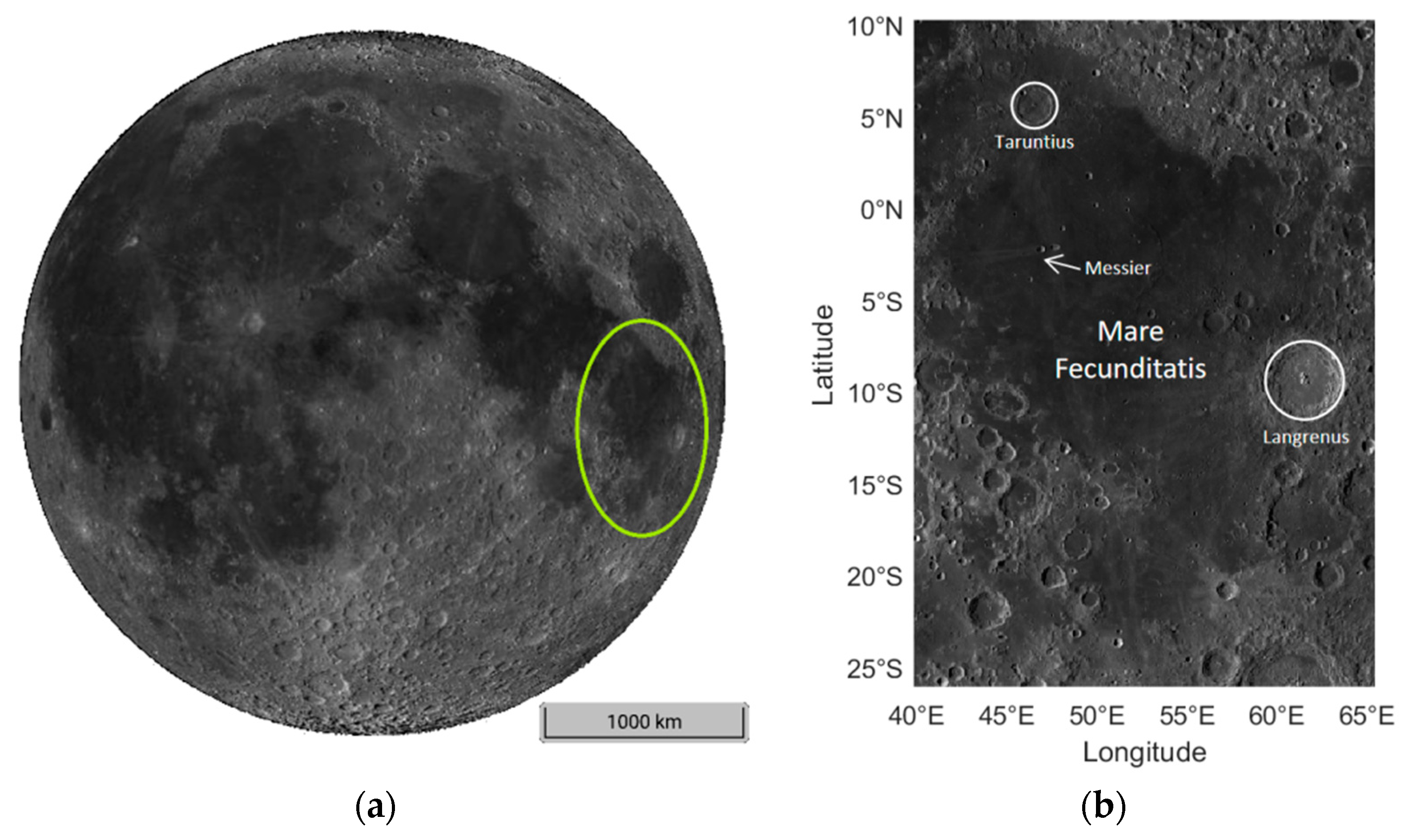
Figure 1. Location and WAC image of Mare Fecunditatis. (a) WAC image of nearside of the Moon, where the location Mare Fecunditatis is indicated by a green ellipse; (b) WAC image of Mare Fecunditatis.
Remotesensing 15 01910 g001
Figure 2. TB and dTB feature maps of Mare Fecunditatis. (a) 3.0 GHz TB features; (b) 7.8 GHz TB features; (c) 19.35 GHz TB features; (d) 37.0 GHz TB features; (1) TBnoon features; (2) TBmidnight features; (3) dTB features.
Remotesensing 15 01910 g002aRemotesensing 15 01910 g002b
Figure 3. Map of Mare Fecunditatis by Kramer et al. in 2008 [30]. Ihtm: high-Ti mare basalt; Chtr: high-Ti spread (regolith); Iltm: low-Ti, mid-Fe HA (high alumina) candidate; Im: low-Ti, low-Fe HA candidate; Cc: obscuring crater ejecta.
Remotesensing 15 01910 g003
Figure 4. Map of labeled study samples.
Remotesensing 15 01910 g004
Figure 5. Overall framework.
Remotesensing 15 01910 g005
Figure 6. Illustration of Random Forest classifier.
Remotesensing 15 01910 g006
Figure 7. Histograms of TB and dTB features for 5 types of sample units in Mare Fecunditatis. (a) 3.0 GHz TB features; (b) 7.8 GHz TB features; (c) 19.35 GHz TB features; (d) 37.0 GHz TB features; (1) TBnoon features; (2) TBmidnight features; (3) dTB features.
Remotesensing 15 01910 g007
Figure 8. Boxplot of TB and dTB features in 5 sample units of Mare Fecunditatis. (a) 3.0 GHz TB features; (b) 7.8 GHz TB features; (c) 19.35 GHz TB features; (d) 37.0 GHz TB features; (1) TBnoon features; (2) TBmidnight features; (3) dTB features.
Remotesensing 15 01910 g008
Figure 9. Pearson coefficient of features.
Remotesensing 15 01910 g009
Figure 10. Pearson coefficient of basalt unit classes.
Remotesensing 15 01910 g010
Figure 11. Normalized ReliefF and OOB importance of all classes.
Remotesensing 15 01910 g011
Figure 12. Random Forest Classification result for all original features.
Remotesensing 15 01910 g012
Figure 13. Contribution rate of each PC.
Remotesensing 15 01910 g013
Figure 14. PCA space of dimension-reduced brightness temperature features. (a) Biplot of the 1st–2nd PCs; (b) Biplot of the 2nd–3rd PCs; (c) Biplot of the 1st–3rd PCs.
Remotesensing 15 01910 g014
Figure 15. Classification results obtained by PCA + RF with different numbers of PCs. (a) Two PCs; (b) Three PCs; (c) Four PCs; (d) Six PCs; (e) Eight PCs; (f) All 12 PCs.
Remotesensing 15 01910 g015
Figure 16. Proportion of each geological unit in Mare Fecunditatis and its vicinity with different methods.
Remotesensing 15 01910 g016
Figure 17. Classification results with features of different frequencies. (a) 3.0 GHz features; (b) 7.8 GHz features; (c) 19.35 GHz features; (d) 37.0 GHz features.
Remotesensing 15 01910 g017
Figure 18. Classification with different acquisition time and dTB features. (a) TBnoon features; (b) TBmidnight features; (c) dTB features.
Remotesensing 15 01910 g018
Table 1. Normalized distance between mare basalt units.
Ihtm-ChtrIhtm-IltmIhtm-CcIhtm-ImChtr-Cc
 TBnoon 3.0 GHz1.76815.29573.89214.63642.2106
 TBmidnight 3.0 GHz0.43592.97010.75082.67620.2153
 TBnoon 7.8 GHz1.33693.57493.71364.12682.8956
 TBmidnight 7.8 GHz0.0360.93220.5051.60140.3954
 TBnoon 19.35 GHz1.36953.97694.30954.63743.4245
 TBmidnight 19.35 GHz0.30770.71971.79360.1491.2652
 TBnoon 37.0 GHz1.15263.584.52454.26963.4361
 TBmidnight 37.0 GHz0.3790.87391.7850.51331.311
 dTB 3.0 GHz0.99733.32573.9564.39362.9824
 dTB 7.8 GHz0.81052.97523.83823.75492.7194
 dTB 19.35 GHz0.97933.27834.3483.88263.4246
 dTB 37.0 GHz0.87632.80733.90623.52372.9714
Chtr-IltmChtr-ImCc-ImCc-IltmIm-Iltm
 TBnoon 3.0 GHz3.20823.43521.68660.62631.3345
 TBmidnight 3.0 GHz1.65392.10642.05171.49521.5721
 TBnoon 7.8 GHz2.7953.53741.17230.0981.0304
 TBmidnight 7.8 GHz0.57651.25831.78581.37581.2378
 TBnoon 19.35 GHz3.03873.89450.85580.35731.1619
 TBmidnight 19.35 GHz0.21490.41741.76451.81950.827
 TBnoon 37.0 GHz2.4713.32640.72140.95471.3622
 TBmidnight 37.0 GHz0.3240.05631.55461.58470.3357
 dTB 3.0 GHz2.43093.36220.17060.27350.4443
 dTB 7.8 GHz1.94282.53580.76820.8830.351
 dTB 19.35 GHz2.27342.88931.01391.58640.7089
 dTB 37.0 GHz1.79452.53560.90931.91561.1222
Table 2. J-S divergence between mare basalt units.
Ihtm-ChtrIhtm-IltmIhtm-CcIhtm-ImChtr-Cc
 TBnoon 3.0 GHz0.62800.69310.69310.69310.6931
 TBmidnight 3.0 GHz0.21660.69310.38600.69310.2027
 TBnoon 7.8 GHz0.57340.69310.69310.69310.6931
 TBmidnight 7.8 GHz0.25600.47740.35500.69310.2791
 TBnoon 19.35 GHz0.61240.69310.69310.69310.6931
 TBmidnight 19.35 GHz0.34630.50610.66750.46100.6143
 TBnoon 37.0 GHz0.61250.69310.69310.69310.6931
 TBmidnight 37.0 GHz0.41940.54900.68140.52260.6344
 dTB 3.0 GHz0.50510.69310.69310.69310.6931
 dTB 7.8 GHz0.55500.69310.69310.69310.6931
 dTB 19.35 GHz0.60590.69310.69310.69310.6931
 dTB 37.0 GHz0.61140.69310.69310.69310.6931
Chtr-IltmChtr-ImCc-ImCc-IltmIm-Iltm
 TBnoon 3.0 GHz0.69310.69310.68720.45560.6291
 TBmidnight 3.0 GHz0.61800.69310.69310.62800.6931
 TBnoon 7.8 GHz0.69310.69310.61080.35190.6086
 TBmidnight 7.8 GHz0.41540.65270.68720.61780.5968
 TBnoon 19.35 GHz0.69310.69310.50520.48630.6233
 TBmidnight 19.35 GHz0.33240.47160.69310.67810.4348
 TBnoon 37.0 GHz0.69310.69310.54770.61460.6321
 TBmidnight 37.0 GHz0.38580.35210.65980.63670.4399
 dTB 3.0 GHz0.69310.69310.20560.30980.3632
 dTB 7.8 GHz0.69310.69310.44250.51390.4346
 dTB 19.35 GHz0.69310.69310.54810.65290.5507
 dTB 37.0 GHz0.68980.69310.57900.68060.6542
Table 3. ReliefF analysis results.
Ihtm-ChtrIhtm-IltmIhtm-CcIhtm-ImChtr-Cc
 TBnoon 3.0 GHz0.26170.60050.52690.58100.3344
 TBmidnight 3.0 GHz0.18340.55390.27900.50170.1079
 TBnoon 7.8 GHz0.10070.46890.49410.51640.3406
 TBmidnight 7.8 GHz0.07430.24920.15040.33220.0847
 TBnoon 19.35 GHz0.12420.50800.53590.54220.4316
 TBmidnight 19.35 GHz0.05600.14880.32600.24370.2063
 TBnoon 37.0 GHz0.08600.46470.54480.52040.4402
 TBmidnight 37.0 GHz0.05410.17240.33480.23040.2431
 dTB 3.0 GHz0.07690.45350.50050.52550.3051
 dTB 7.8 GHz0.04430.42810.48720.50490.2644
 dTB 19.35 GHz0.07540.47110.54910.51980.3946
 dTB 37.0 GHz0.06180.43380.53730.48910.4055
Chtr-IltmChtr-ImCc-ImCc-IltmIm-Iltm
 TBnoon 3.0 GHz0.42020.44670.27700.16030.1775
 TBmidnight 3.0 GHz0.31730.35400.35160.28500.2773
 TBnoon 7.8 GHz0.32720.38670.16650.09220.1008
 TBmidnight 7.8 GHz0.06840.21310.26220.23810.1800
 TBnoon 19.35 GHz0.40490.44870.11300.11220.0981
 TBmidnight 19.35 GHz0.06310.08150.26470.27170.1413
 TBnoon 37.0 GHz0.35250.41060.12090.15280.1280
 TBmidnight 37.0 GHz0.08160.08060.19530.22820.1100
 dTB 3.0 GHz0.26960.34320.09190.08920.1030
 dTB 7.8 GHz0.22430.27130.13040.15450.1164
 dTB 19.35 GHz0.32140.37040.23190.27050.0756
 dTB 37.0 GHz0.29710.34350.16310.26160.1021
Table 4. OOB importance.
Ihtm-ChtrIhtm-IltmIhtm-CcIhtm-ImChtr-Cc
 TBnoon 3.0 GHz1.70610.40620.43380.29200.3154
 TBmidnight 3.0 GHz0.93630.33780.00000.33890.0000
 TBnoon 7.8 GHz0.55350.30980.37770.29360.4470
 TBmidnight 7.8 GHz0.55130.00000.00000.33710.0000
 TBnoon 19.35 GHz0.83810.29340.38180.26060.3538
 TBmidnight 19.35 GHz0.50770.00000.00000.00000.0000
 TBnoon 37.0 GHz0.46380.32330.38090.43260.4071
 TBmidnight 37.0 GHz0.59610.00000.00000.00000.0898
 dTB 3.0 GHz0.51010.36550.39490.43410.3391
 dTB 7.8 GHz0.27830.38020.27600.22350.4152
 dTB 19.35 GHz0.64270.33680.44500.30910.3486
 dTB 37.0 GHz0.45030.39470.29360.35270.3815
Chtr-IltmChtr-ImCc-ImCc-IltmIm-Iltm
 TBnoon 3.0 GHz0.35160.29350.42450.43420.6948
 TBmidnight 3.0 GHz0.08980.40730.62910.59361.5168
 TBnoon 7.8 GHz0.44400.29330.14570.25640.2530
 TBmidnight 7.8 GHz0.00000.00000.51930.28460.5149
 TBnoon 19.35 GHz0.38070.34010.09870.24850.2450
 TBmidnight 19.35 GHz0.00000.00000.80190.86440.2346
 TBnoon 37.0 GHz0.40750.38160.00000.39490.3381
 TBmidnight 37.0 GHz0.09940.00000.30270.53680.2598
 dTB 3.0 GHz0.32380.30890.00000.28070.3729
 dTB 7.8 GHz0.36520.36760.23810.26720.4341
 dTB 19.35 GHz0.52990.43460.13580.81440.1770
 dTB 37.0 GHz0.08980.32440.09890.90410.3668
Disclaimer/Publisher’s Note: The statements, opinions and data contained in all publications are solely those of the individual author(s) and contributor(s) and not of MDPI and/or the editor(s). MDPI and/or the editor(s) disclaim responsibility for any injury to people or property resulting from any ideas, methods, instructions or products referred to in the content.