Hyperspectral Denoising Using Asymmetric Noise Modeling Deep Image Prior

Abstract

Deep image prior (DIP) is a powerful technique for image restoration that leverages an untrained network as a handcrafted prior. DIP can also be used for hyperspectral image (HSI) denoising tasks and has achieved impressive performance. Recent works further incorporate different regularization terms to enhance the performance of DIP and successfully show notable improvements. However, most DIP-based methods for HSI denoising rarely consider the distribution of complicated HSI mixed noise. In this paper, we propose the asymmetric Laplace noise modeling deep image prior (ALDIP) for HSI mixed noise removal. Based on the observation that real-world HSI noise exhibits heavy-tailed and asymmetric properties, we model the HSI noise of each band using an asymmetric Laplace distribution. Furthermore, in order to fully exploit the spatial–spectral correlation, we propose ALDIP-SSTV, which combines ALDIP with a spatial–spectral total variation (SSTV) term to preserve more spatial–spectral information. Experiments on both synthetic data and real-world data demonstrate that ALDIP and ALDIP-SSTV outperform state-of-the-art HSI denoising methods.

1. Introduction

Hyperspectral images (HSIs) are a type of remote sensing data that provide enriched information of the spectral characteristics of a scene. HSIs can be utilized for diverse visual tasks including object detection [1] and classification [2,3,4,5,6,7,8]. However, during the generation and transmission process, the vast amount of HSIs are often corrupted by severe noise, making denoising techniques crucial for effectively analyzing and interpreting the images. Therefore, HSI denoising is vital and has inspired extensive research.

Conventional techniques for HSI denoising, which are often called model-based methods, can be categorized into two groups: filter-based methods and low-rank-based methods. For filter-based methods, 3D model-based methods [9,10] first attempted to take advantage of spatial–spectial information. Then, a variety of methods that utilized penalties to exploit spatial and spectral information [11,12,13,14] were proposed. For low-rank-based methods, they have been found to be more efficient for HSI denoising, and various methods were developed based on low-rank matrix recovery [15,16,17,18,19]. Considering HSI data as a three-order tensor, many low-rank approaches based on tensor decomposition [20,21,22,23] have achieved good effects.

Recently, deep learning has made great progress in a variety of fields. Deep-learning-based denoising methods are regarded as state-of-the-art and many network architectures were proposed for HSI denoising work [24,25,26,27,28]. In refs. [25,27], convolutional-neural-network (CNN)-based architectures were suggested. Generative adversarial networks (GANs) were also examined in [28]. These supervised deep-learning-based methods have a shortcoming that they need a large training set to obtain good effects while HSIs data are limited. To address this issue, a variety of unsupervised methods were developed [29,30,31]. These methods can denoise a single observed HSI without external data.

Among these unsupervised methods, ref. [29] uses deep image prior (DIP) [32] for HSI inverse problems (denoising, inpainting, super-resolution). In ref. [29], 2D convolution was extended to a 3D one, but the 3D one has a poorer performance. However, neither of them is as advanced as most state-of-the-art methods. A popular research trend is to combine DIP with other data priors. For example, reference [30] inserts spatial–spectral total variation (SSTV) into DIP and achieves state-of-the-art results. Despite their good performance, most of the DIP-based methods assume HSIs are corrupted by Gaussian noise or Laplace noise (a.k.a., sparse noise). It is well-known that HSI noise is very complicated, including Gaussian, impulse, stripe and deadline noise. By no means can HSI noise be simply modeled by Gaussian or Laplace noise. How to design a proper noise model for real HSIs plays an important role in HSI denoising and deepens the understanding on the HSI noise pattern. Hence, there is still room to enhance the performance for DIP if it is equipped with more suitable and reasonable noise assumptions.

Our previous work [19] has revealed that synthetic and real-world HSI noise are both heavy-tailed and asymmetric. Taking the Urban dataset as an example, Figure 1 analyzes the statistical distribution of the real-world HSI noise. Band 87, which is degraded by deadline and horizon stripe noise, is shown in Figure 1a. An approximately clean band is generated by averaging bands 85, 86, 87, 88 and 89, as shown in Figure 1b. Finally, the noise of band 87 can be roughly estimated by the observation band minus the corresponding clean one, as displayed in Figure 1c. We thereafter discuss the noise distribution.

Figure 1. Real—world HSI noise analysis. (a) Band 87 of Urban dataset. (b) Generated clean band. (c) Approximate noise of band. (d) Histogram of approximate noise probability density function curves fitted by Laplace distribution and Gaussian distribution, respectively. (e) Histogram of approximate noise and probability density function curve fitted by asymmetric Laplace distribution.

Firstly, traditional DIP’s loss function is mean squared error (MSE, or ${\ell }_2$-norm), which hypothesizes that noise obeys a Gaussian distribution, while Figure 1d demonstrates that the Laplace distribution better fits real-world HSI noise than the Gaussian distribution. This fact suggests that HSI noise is heavy-tailed, so mean absolute error (MAE, or ${\ell }_1$-norm) is the better choice.

Secondly, HSI noise is also asymmetric. For example, the noise frequencies are highly distinct for $n=0.05$ and $n=-0.05$. Neither Gaussian nor Laplace distribution can characterize this property. We propose to utilize an asymmetric Laplace (AL) distribution for modeling real-world HSI noise, and Figure 1e illustrates that the AL distribution is more suitable to characterize the noise, which is both heavy-tailed and asymmetric.

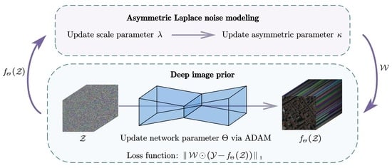
Based on the analysis above, incorporating DIP with the AL distribution assumption may enhance the denoising performance for HSI data. ThereforeInspired by this discovery, an asymmetric Laplace noise modeling deep image prior (ALDIP) method is formulated to boost performance in HSI mixed-noise removal, where the key idea is to assume that the HSI noise of each band obeys an AL distribution. Additionally, to fully utilize spatial–spectral information, we incorporate a spatial–spectral total variation (SSTV) [33] term to preserve the spatial–spectral local smoothness. To validate ALDIP and ALDIP-SSTV’s performance, DIP2D-${\ell }_2$ (2D convolution DIP with ${\ell }_2$ loss), DIP2D-${\ell }_1$ (2D convolution DIP with ${\ell }_1$ loss), ALDIP, ALDIP-SSTV are applied to the real-world HSI dataset Shanghai. The result is displayed in Figure 2.

Figure 2. Comparison of DIP2D-${\ell }_2$ (2D convolution DIP with ${\ell }_2$ loss) and DIP2D-${\ell }_1$ (2D convolution DIP with ${\ell }_1$ loss) on the real-world HSI Shanghai dataset. Two local areas (red and blue squares) are demarcated zoomed for easy observation. (a) Real-world noisy HSI Shanghai (The enhanced pseudo images consisted of the 152nd, 89th and 43rd bands). (b) DIP2D-${\ell }_2$ method denoising result. (c) DIP2D-${\ell }_1$ denoising result. (d) ALDIP method denoising result. (e) ALDIP-SSTV method denoising result.

According to Figure 2, it is evident that ALDIP and ALDIP-SSTV preserve more details than DIP2D-${\ell }_2$ and DIP2D-${\ell }_1$. This confirms our analysis of HSI noise and shows that modeling HSI noise as an asymmetric Laplace distribution provides superior results for HSI mixed noise removal. Furthermore, we compare ALDIP and ALDIP-SSTV with other state-of-the-art methods on two synthetic and three real-world HSI datasets. The result shows that ALDIP and ALDIP-SSTV outperform other methods. The main contributions of this paper can be formulated as follows:

• We propose ALDIP for HSI mixed noise removal. More specifically, we combine a more suitable and reasonable noise model with DIP. Our model hypothesizes real-world HSI noise obeys asymmetric Laplace (AL) distribution.
• ALDIP-SSTV is presented by incorporating the SSTV term to fully utilize spatial–spectral information for performance improvement.
• A variety of experiments are conducted that rigorously validate the effectiveness of our methods. The result shows that our methods outperform many state-of-the-art methods.

The rest of this paper is structured as follows: Section 2 contains a brief overview of the related work. Section 3 introduces the methods we propose. Section 4 introduces the experiments we conduct. Finally, Section 5 concludes the paper.

2. Related Works

2.1. Low-Rank Models for HSI Denoising

As is known, HSIs contain high correlations in the spectral dimension and clean HSIs tend to have many minor singular values, which means clean HSIs are mostly low-rank. For a HSI with B bands and $M\times N$ pixels denoted by $\mathbf{Y}\in {\mathbb{R}}^{MN\times B}$, the low-rank matrix factorization (LRMF) is modeled as follows:

$$\underset{\mathbf{U}\in {\mathbb{R}}^{MN\times R},\mathbf{V}\in {\mathbb{R}}^{B\times R}}{min}{\parallel \mathbf{Y}-\mathbf{U}{\mathbf{V}}^{\top }\parallel }_2^2,$$

(1)

where $\mathbf{U}$ and $\mathbf{V}$ are of rank R. Singular value decomposition (SVD) [34] can solve Equation (1). The above model hypothesizes noise obeys the Gaussian distribution while real-world HSI noise is complicated. To achieve higher robustness, modeling can be approached from another perspective. We assume that a noisy HSI $\mathbf{Y}$ can be regarded as a combination of a low-rank clean HSI $\mathbf{X}$ and unknown sparse noise $\mathbf{S}$, i.e.,

$$\mathbf{Y}=\mathbf{X}+\mathbf{S}.$$

(2)

Robust principal component analysis (RPCA) can be utilized to recover low-rank clean HSI $\mathbf{X}$ and sparse noise $\mathbf{S}$ from $\mathbf{Y}$, and the corresponding optimization issue is written as

$$\underset{\mathbf{X},\mathbf{S}}{min}{\parallel \mathbf{X}\parallel }_{*}+\lambda {\parallel \mathbf{S}\parallel }_1, \mathrm{s}.\mathrm{t}.\mathbf{Y}=\mathbf{X}+\mathbf{S},$$

(3)

where ${\parallel ·\parallel }_{*}$ denotes the nuclear norm of a matrix and $\lambda$ denotes the parameter for regularization terms. Ref. [16] utilized the above model to recover HSIs and performed well when removing Gaussian noise, impulse noise, deadlines and stripes.

Besides LRMF and RPCA, tensor decomposition algorithms including Tucker and CANDECOMP/PARAFAC (CP) [34] have been developed [21,22,23,35] by regarding the HSI data cube as a three-order tensor, and have made a remarkable achievement on HSI denoising.

Low-rank denoising methods can be improved by adding different regularizations. To preserve more spatial details, the non-local similarity (NLS) property is widely combined with low-rank models [34,36,37]. Total variation regularization can help keep local smoothness to a certain degree. It has been widely used in low-rank-based methods [22,38,39]. A TV-regularized low-rank (LRTV) matrix factorization method [39] was proposed and has impressive performance.

2.2. Deep Learning Based Methods for HSI Denoising

Deep-learning-based methods have shown great promise in HSI denoising. It has been proved that convolutional neural networks (CNNs) can approximate any complex, non-linear relationships between the input and output data [40], which indicates that CNNs can handle complicated mixed noise. Ref. [28] first introduces CNNs in HSI denoising, which uses 2D filters to capture spatial and spectral structures. In ref. [41], two parallel branches for feature extraction are used to obtain spatial and spectral information. To further exploit the spectral correlations, a 3D U-net is proposed for HSI denoising [24]. With regard to the directivity and spectral difference of the spatial structure, Ref. [42] is proposed for HSI mixed noise removal. Refs. [43,44,45,46] utilize attention to reduce redundant information.

Although deep-learning-based methods have state-of-the-art performance, they depend on large amounts of data. Paired real-world HSIs are limited and difficult to obtain while models trained on synthetic data are difficult to generalize to real data.

2.3. Noise Modeling for HSI Denoising

Noise modeling in denoising tasks can be regarded as a type of prior knowledge. For HSI denoising, the insightful understanding towards noise distribution provides valuable information to better remove the noise and preserve the underlying clean signal.

Most methods simply model HSI noise as a Gaussian distribution. In this case, ${\ell }_2$ norm is used for the fidelity term. This can simplify the optimization problem and make it more tractable. However, in most cases, it may not accurately reflect the complicated mixed noise in real-world HSIs.

Complex mixed HSI noise can be modeled as a mixture of Gaussians (MoG), which can approximate any continuous distributions. Based on this theory, ref. [47] developed MoG-LRMF. In the following works, MoG is combined with low-rank tensor decomposition [48,49,50]. However, the MoG’s universal approximation property holds only if the number of Gaussian components increases to an infinite amount, which is not feasible in real-world applications. Refs. [51,52] model unknown noise as a mixture of exponential power distributions (MoEP), which alleviates MoG’s limitations. These methods are based on independent and identically distributed (i.i.d.) noise assumptions, so they neglect diverse noise patterns for different bands. The non-i.i.d. MoG (NMoG) proposed in [50] breaks through this bottleneck by assigning all bands with different forms of MoG noise.

The asymmetry of HSI noise is ignored in the above noise modeling methods. In ref. [19], HSI noise is modeled as an AL distribution and they proposed a bandwise-AL-noise-based matrix factorization (BALMF) method for achieving better performance.

2.4. Deep Image Prior

The recent work by [32] is an unsupervised deep-learning-based method. It found that the structure of a generator network can be used as a handcrafted prior to solve standard inverse problems, e.g., denoising and inpainting. The knowledge implicit contained in the network is called deep image prior (DIP). Hereafter, ref. [29] applied DIP to HSI restoration. In ref. [29], 2D convolution was extended to a 3D one, but the 3D one has poorer performance.

DIP for HSI solves the following optimization problem:

$$\underset{\theta }{min}{\parallel f_{\theta }\left(z\right)-x_0\parallel }_2^2,$$

(4)

where z is a randomly sampled input, $x_0$ is a corrupted image, and f is a CNN with parameters $\theta$. The restored result is

$$x^{*}=f_{{\theta }^{*}}\left(z\right),\mathrm{where}{\theta }^{*}=\underset{\theta }{argmin}{\parallel f_{\theta }\left(z\right)-x_0\parallel }_2^2.$$

(5)

Apparently, the optimization will eventually result in a degraded image, which is the same as $x_0$. Ref. [32] found that the CNN will learn the signal first and learn noise slowly. Therefore, the number of iterations is restricted to a certain number. This operation is called early stopping.

To improve the performance of DIP, many studies have incorporated various regularization terms into the loss function [53,54,55]. For HSI denoising, ref. [30] incorporates a spatial–spectral total variation (SSTV) term to preserve the spatial–spectral local smoothness of HSI.

3. Proposed Model

3.1. Model Formulation

Given a noisy HSI with B bands and $M\times N$ pixels denoted by $\mathcal{Y}\in {\mathbb{R}}^{M\times N\times B}$, it can be considered as a clean HSI $\mathcal{X}\in {\mathbb{R}}^{M\times N\times B}$ plus the mixed noise $\mathcal{N}\in {\mathbb{R}}^{M\times N\times B}$, which can be formulated as follows:

$$\mathcal{Y}=\mathcal{X}+\mathcal{N}.$$

(6)

For each pixel, it can be formulated as

$${\mathcal{Y}}_{i,j,k}={\mathcal{X}}_{i,j,k}+{\mathcal{N}}_{i,j,k},$$

(7)

where ${\mathcal{Y}}_{i,j,k},{\mathcal{X}}_{i,j,k}$ and ${\mathcal{N}}_{i,j,k}$ denote the $(i,j,k)$-th element of $\mathcal{Y},\mathcal{X}$ and $\mathcal{N}$, respectively.

To effectively characterize the self-similarity of HSIs, we employ the DIP method. Specifically, based on Equation (5), a clean HSI $\mathcal{X}$ can be generated by a network:

$$\mathcal{X}=f_{\mathrm{\Theta }}\left(\mathcal{Z}\right),$$

(8)

where $\mathrm{\Theta }$ is the parameters of network and $\mathcal{Z}\in {\mathbb{R}}^{M\times N\times B}$ is the network input, which is randomly sampled from $\mathrm{Uniform}(0,0.1)$. This form implicitly contains the prior captured by the neural network.

According to the loss function in Equation (4), the DIP model only considers the Gaussian noise. To overcome this drawback, we assume the HSI noise of each band obeys an AL distribution. In more detail, we consider that the real-world HSI noise of each band is different, but is distributed as the same kind of distribution. Mathematically, there is

$${\mathcal{N}}_{i,j,k}\sim {\mathrm{AL}}_k\left({\mathcal{N}}_{i,j,k}|0,{\lambda }_k,{\kappa }_k\right),\forall k=1,2,\cdots ,B,$$

(9)

where ${\lambda }_k$ and ${\kappa }_k$ are the k-th element of $\lambda$ and $\kappa$, respectively. The probability density function (pdf) of AL is as

$$f_{\mathrm{AL}}(x,\mu ,\lambda ,\kappa )=\lambda \kappa (1-\kappa )exp\left(-|x-\mu |\lambda \eta \right),$$

(10)

where $-inf<\mu <inf$ is the location parameter, $\lambda >0$ is the scale parameter and $0<\kappa <1$ is the skew parameter. $\eta =\kappa \mathbb{I}(x⩾\mu )+(1-\kappa )\mathbb{I}(x<\mu )$ and $\mathbb{I}\left(e\right)$ is the indicator function defined as follows:

$$\mathbb{I}\left(e\right)=\left\{\begin{array}{cc}1\hfill & \mathrm{if}e\mathrm{is}\mathrm{true}\hfill \\ 0\hfill & \mathrm{if}e\mathrm{is}\mathrm{false}.\hfill \end{array}\right.$$

(11)

According to Equations (7) and (9), each pixel of noisy HSI $\mathcal{Y}$ has the following distribution:

$${\mathcal{Y}}_{i,j,k}\sim {\mathrm{AL}}_k\left({\mathcal{Y}}_{i,j,k}|{\mathcal{X}}_{i,j,k},{\lambda }_k,{\kappa }_k\right),\forall k=1,2,\cdots ,B.$$

(12)

Given this assumption, the log-likelihood function can be written as follows:

$$\begin{array}{cc}\hfill l(\mathcal{X},\lambda ,\kappa )& =\sum _{i,j,k}log{\mathrm{AL}}_k\left({\mathcal{Y}}_{i,j,k}|{\mathcal{X}}_{i,j,k},{\lambda }_k,{\kappa }_k\right)\hfill \\ \hfill & =\sum _{i,j,k}-|{\mathcal{Y}}_{i,j,k}-{\mathcal{X}}_{i,j,k}|{\lambda }_k{\eta }_{i,j,k}+log\left({\lambda }_k{\kappa }_k(1-{\kappa }_k)\right)\hfill \\ \hfill & =-\parallel \mathcal{W}\odot \left(\mathcal{Y}-\mathcal{X}\right){\parallel }_1+MN\sum _{k=1}^{B}log\left({\lambda }_k{\kappa }_k(1-{\kappa }_k)\right),\hfill \end{array}$$

(13)

where the $(i,j,k)$-th element of $\mathcal{W}$ is defined by ${\mathcal{W}}_{i,j,k}={\lambda }_k{\eta }_{i,j,k}={\lambda }_k\left({\kappa }_k\mathbb{I}({\mathcal{Y}}_{i,j,k}⩾{\mathcal{X}}_{i,j,k})+(1-{\kappa }_k)\mathbb{I}({\mathcal{Y}}_{i,j,k}<{\mathcal{X}}_{i,j,k})\right)$.

According to the maximum likelihood estimation (MLE) principle, the parameters $\mathrm{\Theta },\lambda$ and $\kappa$ can be iteratively updated by maximizing the likelihood function $\ell (\mathcal{X},\lambda ,\kappa )$. Therefore, the optimization model is as follows:

$$\begin{array}{cc}\hfill \underset{\mathrm{\Theta },\lambda ,\kappa }{min}& \parallel \mathcal{W}\odot \left(\mathcal{Y}-\mathcal{X}\right){\parallel }_1-MN\sum _{k=1}^{B}log\left({\lambda }_k{\kappa }_k(1-{\kappa }_k)\right)\hfill \\ \hfill \mathrm{s}.\mathrm{t}. & \mathcal{X}=f_{\mathrm{\Theta }}\left(\mathcal{Z}\right).\hfill \end{array}$$

(14)

After removing the equality constraint, the issue is cast as the following problem:

$$\underset{\mathrm{\Theta },\lambda ,\kappa }{min}\parallel \mathcal{W}\odot \left(\mathcal{Y}-f_{\mathrm{\Theta }}\left(\mathcal{Z}\right)\right){\parallel }_1-MN\sum _{k=1}^{B}log\left({\lambda }_k{\kappa }_k(1-{\kappa }_k)\right).$$

(15)

To further preserve the spatial–spectral local smoothness, we incorporate a spatial–spectral total variation (SSTV) term for an ALDIP model. The SSTV term is shown below:

$${\parallel \mathcal{X}\parallel }_{\mathrm{SSTV}}=\parallel D_h{\mathcal{X}D\parallel }_1+{\parallel D_v\mathcal{X}D\parallel }_1,$$

(16)

where $D_h$ and $D_v$ are horizontal and vertical 2D finite differencing operators, respectively. D is a 1D finite differencing operator on the spectral signature of each pixel. After incorporating the SSTV term to ALDIP, we will have the ALDIP-SSTV model as:

$$\underset{\mathrm{\Theta },\lambda ,\kappa }{min}\parallel \mathcal{W}\odot \left(\mathcal{Y}-f_{\mathrm{\Theta }}\left(\mathcal{Z}\right)\right){\parallel }_1-MN\sum _{k=1}^{B}log\left({\lambda }_k{\kappa }_k(1-{\kappa }_k)\right)+\tau {\parallel f_{\mathrm{\Theta }}\left(\mathcal{Z}\right)\parallel }_{\mathrm{SSTV}},$$

(17)

where $\tau$ is the parameter for the SSTV term.

3.2. Solving Algorithm

For ALDIP (Equation (15)) and ALDIP-SSTV (Equation (17)), the solving algorithms are similar. The following derivation is based on ALDIP-SSTV. The loss function of ALDIP-SSTV is as the following:

$$L(\mathrm{\Theta },\lambda ,\kappa )=\parallel \mathcal{W}\odot \left(\mathcal{Y}-f_{\mathrm{\Theta }}\left(\mathcal{Z}\right)\right){\parallel }_1-MN\sum _{k=1}^{B}log\left({\lambda }_k{\kappa }_k(1-{\kappa }_k)\right)+\tau {\parallel f_{\mathrm{\Theta }}\left(\mathcal{Z}\right)\parallel }_{\mathrm{SSTV}}.$$

(18)

The parameters of AL noise ($\lambda$ and $\kappa$) and network ($\mathrm{\Theta }$) can be iteratively updated by minimizing Equation (18).

Updating $\mathbf{\lambda }$: The loss function with respect to $\lambda$ is written as:

$$L\left(\lambda \right)=\parallel \mathcal{W}\odot \left(\mathcal{Y}-f_{\mathrm{\Theta }}\left(\mathcal{Z}\right)\right){\parallel }_1-MN\sum _{k=1}^{B}log{\lambda }_k.$$

(19)

For ${\lambda }_k,k=1,2,\cdots ,B$, the loss function is shown as:

$$L\left({\lambda }_k\right)={\lambda }_k\sum _{i,j}{\eta }_{i,j,k}|{\mathcal{Y}}_{i,j,k}-f_{\mathrm{\Theta }}{\left(\mathcal{Z}\right)}_{i,j,k}|-MN\sum _{k=1}^{B}log{\lambda }_k.$$

(20)

The gradient of the above equation can be obtained as follows:

$$\frac{\partial L\left({\lambda }_k\right)}{\partial {\lambda }_k}=\sum _{i,j}{\eta }_{i,j,k}|{\mathcal{Y}}_{i,j,k}-f_{\mathrm{\Theta }}{\left(\mathcal{Z}\right)}_{i,j,k}|-\frac{MN}{{\lambda }_k}.$$

(21)

Let Equation (21) be zero, and the updating formula can be obtained as follows:

$${\lambda }_k=\frac{MN}{{\sum }_{i,j}{\eta }_{i,j,k}|{\mathcal{Y}}_{i,j,k}-f_{\mathrm{\Theta }}{\left(\mathcal{Z}\right)}_{i,j,k}|},k=1,2,\cdots ,B$$

(22)

Updating $\mathbf{\kappa }$: The loss function with regard to ${\kappa }_j$ is

$$L\left({\kappa }_k\right)={\lambda }_k\sum _{i,j}{\eta }_{i,j,k}|{\mathcal{Y}}_{i,j,k}-f_{\mathrm{\Theta }}{\left(\mathcal{Z}\right)}_{i,j,k}|-MN\sum _{k=1}^{B}log\left({\kappa }_k(1-\kappa )\right).$$

(23)

For ${\eta }_{i,j,k}$, take the partial derivative with respect to ${\kappa }_k$:

$$\begin{array}{cc}\hfill \frac{\partial {\eta }_{i,j,k}}{\partial {\kappa }_k}& =\frac{\partial \left({\kappa }_k\mathbb{I}({\mathcal{Y}}_{i,j,k}-f_{\mathrm{\Theta }}{\left(\mathcal{Z}\right)}_{i,j,k}⩾0)+(1-{\kappa }_k)\mathbb{I}({\mathcal{Y}}_{i,j,k}-f_{\mathrm{\Theta }}{\left(\mathcal{Z}\right)}_{i,j,k}<0)\right)}{\partial {\kappa }_k}\hfill \\ \hfill & =\mathbb{I}({\mathcal{Y}}_{i,j,k}-f_{\mathrm{\Theta }}{\left(\mathcal{Z}\right)}_{i,j,k}⩾0)-\mathbb{I}({\mathcal{Y}}_{i,j,k}-f_{\mathrm{\Theta }}{\left(\mathcal{Z}\right)}_{i,j,k}<0)\hfill \\ \hfill & =\mathrm{sign}({\mathcal{Y}}_{i,j,k}-f_{\mathrm{\Theta }}{\left(\mathcal{Z}\right)}_{i,j,k}).\hfill \end{array}$$

(24)

Thus, the gradient of Equation (23) is written as follows:

$$\frac{\partial L\left({\kappa }_k\right)}{\partial {\kappa }_k}={\lambda }_k\sum _{i,j}\left({\mathcal{Y}}_{i,j,k}-f_{\mathrm{\Theta }}{\left(\mathcal{Z}\right)}_{i,j,k}\right)-\frac{MN}{{\kappa }_k}+\frac{MN}{1-{\kappa }_k}.$$

(25)

Let the above equation be zero, and we can obtain the following quadratic equation:

$${\xi }_k{\kappa }_k^2-({\xi }_k+2MN){\kappa }_k+MN=0,$$

(26)

where ${\xi }_k={\lambda }_k{\sum }_{i,j}\left({\mathcal{Y}}_{i,j,k}-f_{\mathrm{\Theta }}{\left(\mathcal{Z}\right)}_{i,j,k}\right)$. This quadratic equation can be solved directly using the quadratic formula. The following root satisfies the constraint $0<\kappa <1$ [19]:

$${\kappa }_k=\frac{{\xi }_k+2MN-\sqrt{{\xi }_k^2+4M^2{N}^2}}{2{\xi }_k},k=1,2,\cdots ,B.$$

(27)

Updating $\mathrm{\Theta }$: After updating the parameters of AL noise model $\lambda$ and $\kappa$, we update the network parameter $\mathrm{\Theta }$. The loss function with respect to $\mathrm{\Theta }$ is

$$L\left(\mathrm{\Theta }\right)=\parallel \mathcal{W}\odot (\mathcal{Y}-f_{\mathrm{\Theta }}\left(\mathcal{Z}\right)){\parallel }_1+\tau {\parallel f_{\mathrm{\Theta }}\left(\mathcal{Z}\right)\parallel }_{\mathrm{SSTV}}.$$

(28)

Adaptive moment estimation (ADAM) algorithm is used for this step, which includes momentum and bias correction terms to accelerate the learning process and stabilize the updates.

The solving algorithm is summarized in Algorithm 1.

Algorithm 1: ALDIP or ALDIP-SSTV.

4. Experiments

To validate the effectiveness and performance of ALDIP and ALDIP-SSTV, we conduct experiments on both synthetic and real-world HSI data. To further demonstrate the superiority of our methods, following eight state-of-the-art methods are selected for comparison:

• Low-rank methods: fast hyperspectral denoising (FastHyDe) [56], which is based on low-rank and sparse representations.
• TV regularized low-rank methods: TV regularized low-rank matrix factorization (LRTV) [39] and TV regularized low-rank tensor decomposition (LRTDTV) [22], and three-dimensional correlated total variation regularized RPCA (CTV) [57].
• Noise modeling methods: non-i.i.d. mixture of Gaussians modeling low-rank matrix factorization (NMoG) [50] and a bandwise-AL-noise-based matrix factorization (BALMF) [19].
• DIP-based methods: 2D convolution DIP with ${\ell }_2$ loss (DIP2D-${\ell }_2$) [29], 2D convolution DIP with ${\ell }_1$ loss (DIP2D-${\ell }_1$) [29] and spatial–spectral constrained unsupervised deep image prior (S2DIP) [30].

In this paper, we use a four-layer hourglass architecture with skip connections, which is shown in Figure 3. We use the Adam optimizer with a learning rate of 0.01 for the network in the following experiments.

Figure 3. Network architecture used for experiments.

4.1. Synthetic Data Experiment

Two HSI datasets are selected to conduct the simulated denoising experiment:

• Indian Pines: ground truth of the scene gathered by AVIRIS sensor over the Indian Pines test site in north-western Indiana with $145\times 145$ pixels and 224 bands.
• Pavia Centre: a cropped HSI with 200 × 200 pixels and 80 bands acquired by the ROSIS sensor during a flight campaign over Pavia, northern Italy.

To simulate real-world HSI noise, we firstly set up eight different noise cases that synthesize various types of noise ranging from simple to complex. Furthermore, four more cases are set up to simulate the scenario where the signal is more severely corrupted by mixed noise. On the basis of case 8, these four cases simulate more severe mixture noise either by adding more severe noise (case 9, case 10) or by having more bands corrupted (case 11, case 12). Table 1 shows the details of the synthetic noise setting. Cases 3 to 12 are more consistent with real-world HSI noise.

Table 1. Synthetic noise setting. $\sigma$ denotes the standard deviation of Gaussian noise. p denotes the sampling rate of impulse noise. q is the number of deadlines and stripes.

Case	Gaussian Noise		Impulse Noise		Deadline		Stripe
	Bands	$\mathit{\sigma }$	Bands	p	Bands	q	Bands	q
Case 1	all bands	0.05	-	-	-	-	-	-
Case 2	all bands	0.01∼0.05 *	-	-	-	-	-	-
Case 3	all bands	0.01	all bands	$p=$ 0.1	-	-	-	-
Case 4	all bands	0.01	all bands	$p=$ 0.1	10% bands	$q=$ 35	-	-
Case 5	all bands	0.01	all bands	$p=$ 0.1	20% bands	$q=$ 35	20% bands	$q=$ 35
Case 6	all bands	0.01	all bands	$p=$ 0.15	30% bands	$q=$ 35	30% bands	$q=$ 35
Case 7	all bands	0.01	all bands	$p=$ 0.25	40% bands	$q=$ 35	40% bands	$q=$ 35
Case 8	all bands	0.01	all bands	$p=$ 0.3	50% bands	$q=$ 35	50% bands	$q=$ 35
Case 9	all bands	0.01	all bands	$p=$ 0.35	50% bands	$q=$ 40	50% bands	$q=$ 40
Case 10	all bands	0.01	all bands	$p=$ 0.4	50% bands	$q=$ 45	50% bands	$q=$ 45
Case 11	all bands	0.01	all bands	$p=$ 0.3	60% bands	$q=$ 35	60% bands	$q=$ 35
Case 12	all bands	0.01	all bands	$p=$ 0.3	70% bands	$q=$3 5	70% bands	$q=$ 35

* In case 2, each band is corrupted by Gaussian noise with $\sigma$ randomly sampled from 0.01 to 0.05.

For fair comparison, the hyper-parameters for all methods are fine-tuned to achieve their best performance and metrics for evaluation include: PSNR (Peak Signal-to-Noise Ratio), SSIM (Structural Similarity), SAM (Spectral Angle Mapper) and ERGAS (Erreur Relative Global Adimensionnelle de Synthèse).

Table 2 and Table 3 present the evaluation results for the twelve cases on the Indian Pines and Pavia Centre datasets. We will analyze the experiment results to gain a deeper understanding of the performance of our model.

Table 2. The metrics of a synthetic data experiment on HSI dataset Indian Pines. The optimal values are indicated in bold and the second-best values are underlined.

Cases	Metrics	Noisy	FastHyDe	LRTV	LRTDTV	NMoG	BALMF	CTV	DIP2D-${\mathit{\ell }}_2$	DIP2D-${\mathit{\ell }}_1$	S2DIP	ALDIP	ALDIP-SSTV
Case 1	PSNR	26.03	39.23	43.76	43.44	39.05	36.13	40.08	41.04	40.10	44.91	40.10	41.84
	SSIM	0.6036	0.9590	0.9929	0.9956	0.9583	0.9092	0.9721	0.9780	0.9699	0.9971	0.9669	0.9816
	SAM	5.8973	1.1306	0.6230	0.6513	1.2091	1.7804	1.05	0.8983	0.9976	0.6930	0.9892	0.7755
	ERGAS	116.62	26.80	16.08	17.16	27.32	37.87	24.41	21.18	23.74	15.70	23.66	20.46
Case 2	PSNR	30.84	41.78	47.28	44.80	44.10	39.98	42.25	44.67	44.05	47.02	46.03	47.07
	SSIM	0.7569	0.9812	0.9968	0.9973	0.9865	0.9561	0.9812	0.9904	0.9888	0.9981	0.9921	0.9947
	SAM	3.9517	0.8090	0.3974	0.5323	0.6781	1.2462	0.862	0.5932	0.6510	0.5345	0.5022	0.4529
	ERGAS	78.13	20.29	11.09	15.24	15.61	26.88	19.56	14.01	15.15	12.42	12.12	11.39
Case 3	PSNR	18.52	28.06	48.47	44.62	46.80	47.19	47.84	30.46	49.45	48.11	49.82	50.40
	SSIM	0.4557	0.8076	0.9988	0.9980	0.9948	0.9947	0.9944	0.9133	0.9978	0.9993	0.9980	0.9984
	SAM	13.1936	2.7764	0.2494	0.4344	0.3999	0.4128	0.4319	1.8306	0.3375	0.2903	0.3218	0.3047
	ERGAS	273.80	92.08	8.96	15.68	16.75	11.03	10.24	69.44	8.74	9.41	7.86	7.48
Case 4	PSNR	17.10	24.74	37.09	39.96	35.24	41.96	44.11	30.27	48.99	48.06	49.76	50.31
	SSIM	0.4073	0.7181	0.9655	0.9845	0.9809	0.9743	0.9692	0.9061	0.9978	0.9992	0.9979	0.9982
	SAM	17.9269	8.6414	2.8213	1.5948	5.6250	3.6964	1.5977	1.9643	0.2914	0.2979	0.3245	0.3057
	ERGAS	371.64	213.74	75.18	45.80	117.76	87.57	36.52	70.96	8.35	9.47	7.89	7.50
Case 5	PSNR	16.89	24.59	36.78	39.45	36.01	41.19	41.23	29.77	48.00	47.72	48.81	49.62
	SSIM	0.3937	0.7089	0.9602	0.9792	0.9805	0.9662	0.9354	0.8975	0.9972	0.9991	0.9977	0.9981
	SAM	18.3366	8.7609	3.0209	1.6783	5.3124	3.2847	2.8146	2.3404	0.3566	0.3564	0.3558	0.3234
	ERGAS	377.49	217.16	81.72	51.00	111.17	84.29	61.26	76.72	10.06	10.31	9.28	8.18
Case 6	PSNR	16.06	22.94	36.18	38.91	40.04	39.93	37.91	29.72	47.24	47.55	48.66	49.54
	SSIM	0.3622	0.6569	0.9584	0.9817	0.9830	0.9592	0.9880	0.8838	0.9968	0.9990	0.9973	0.9980
	SAM	20.8171	10.6067	2.5872	1.5086	5.0481	3.8595	1.0938	2.6751	0.4134	0.3835	0.3713	0.3334
	ERGAS	423.77	258.33	76.07	48.55	106.80	88.84	36.42	77.99	10.98	10.39	9.24	8.25
Case 7	PSNR	15.30	21.85	34.35	37.80	39.61	37.16	36.63	29.63	46.30	47.03	48.11	49.71
	SSIM	0.3310	0.6335	0.9457	0.9763	0.9845	0.9369	0.9857	0.8871	0.9960	0.9987	0.9966	0.9975
	SAM	22.6722	11.0750	3.3362	1.3765	4.5066	3.9360	1.1551	2.9089	0.4594	0.4495	0.3846	0.3577
	ERGAS	461.45	278.01	84.80	43.50	94.44	98.32	40.56	80.22	12.44	11.48	9.77	8.37
Case 8	PSNR	14.52	19.96	32.80	36.49	39.31	35.02	35.66	29.18	46.01	46.61	47.95	49.32
	SSIM	0.3012	0.5566	0.9300	0.9750	0.9849	0.9128	0.9838	0.8668	0.9959	0.9985	0.9969	0.9973
	SAM	24.6293	13.6830	3.2331	1.3849	4.3261	3.2084	1.2382	3.2743	0.4792	0.4933	0.4013	0.3914
	ERGAS	497.95	323.77	89.67	51.52	92.30	94.75	44.59	85.39	12.86	12.28	9.95	9.19
Case 9	PSNR	14.29	19.70	28.54	33.94	34.15	33.31	34.65	28.81	44.48	46.08	47.10	50.20
	SSIM	0.2916	0.6960	0.9171	0.9444	0.9216	0.8749	0.9811	0.8525	0.9937	0.9981	0.9962	0.9981
	SAM	25.6182	12.3029	4.7091	2.6407	8.0042	5.0992	1.2395	3.6646	0.6310	0.5571	0.4811	0.3556
	ERGAS	518.06	313.29	123.04	80.01	180.95	132.82	48.79	91.31	16.00	13.39	11.94	8.18
Case 10	PSNR	14.08	19.12	27.13	31.01	29.21	29.56	33.66	28.84	42.70	46.14	46.99	49.79
	SSIM	0.2831	0.6754	0.8783	0.9047	0.8376	0.8267	0.9777	0.8502	0.9919	0.9983	0.9959	0.9978
	SAM	26.8287	13.9469	5.8248	4.0121	10.7548	7.0674	1.4748	3.7119	0.7584	0.5570	0.4909	0.3923
	ERGAS	538.55	342.07	139.38	107.30	259.88	167.56	55.69	91.63	20.07	13.53	12.52	9.32
Case 11	PSNR	13.80	18.62	31.58	34.60	37.87	32.87	35.23	27.67	43.95	45.67	47.37	48.79
	SSIM	0.2796	0.5233	0.9714	0.9615	0.9811	0.9003	0.9821	0.8369	0.9936	0.9982	0.9956	0.9972
	SAM	26.4903	14.6744	2.3998	2.0343	5.0204	4.4053	1.2945	3.9564	0.6378	0.5478	0.4563	0.4067
	ERGAS	531.88	349.84	79.30	63.94	104.89	108.83	47.07	101.46	16.17	13.65	10.70	9.56
Case 12	PSNR	13.14	17.55	31.01	33.62	35.51	31.37	34.6	27.31	43.29	45.44	45.54	48.05
	SSIM	0.2576	0.4994	0.9706	0.9600	0.9657	0.8594	0.9804	0.8235	0.9931	0.9982	0.9949	0.9966
	SAM	28.0145	15.0541	2.4515	2.1039	6.0969	4.8016	1.4321	4.0036	0.6207	0.5570	0.4942	0.4582
	ERGAS	561.12	372.75	79.56	65.50	131.85	122.80	50.42	103.93	17.03	13.88	13.13	11.05

Table 3. The metrics of a synthetic data experiment on the HSI dataset Pavia Centre. The optimal values are indicated in bold and the second-best values are underlined.

Cases	Metrics	Noisy	FastHyDe	LRTV	LRTDTV	NMoG	BALMF	CTV	DIP2D-${\mathit{\ell }}_2$	DIP2D-${\mathit{\ell }}_1$	S2DIP	ALDIP	ALDIP-SSTV
Case 1	PSNR	26.30	39.20	39.48	35.86	39.51	37.43	38.8	39.17	39.00	40.04	37.45	38.69
	SSIM	0.7424	0.9800	0.9829	0.9620	0.9811	0.9680	0.9794	0.9809	0.9805	0.9845	0.9814	0.9840
	SAM	17.0067	3.7325	3.8531	4.6013	3.5918	5.3550	3.7128	3.7796	4.0133	3.0926	4.3570	4.0333
	ERGAS	175.10	40.62	39.03	58.34	39.22	50.16	41.83	40.37	41.22	36.22	49.91	43.81
Case 2	PSNR	31.65	41.78	42.08	37.46	44.68	41.65	41.78	41.98	42.59	43.80	43.47	44.10
	SSIM	0.8729	0.9902	0.9912	0.9734	0.9938	0.9868	0.9902	0.9891	0.9907	0.9928	0.9943	0.9949
	SAM	12.1869	3.0119	3.0857	4.0471	2.5040	3.9117	2.7267	3.2144	2.9836	2.4591	2.5291	2.4204
	ERGAS	113.60	30.25	29.25	49.42	22.24	33.56	30.44	29.99	27.94	23.97	25.83	24.08
Case 3	PSNR	22.36	35.48	43.90	38.49	47.64	46.40	42.71	35.64	47.25	47.43	46.36	47.29
	SSIM	0.6967	0.9662	0.9948	0.9806	0.9970	0.9964	0.9942	0.9673	0.9967	0.9969	0.9974	0.9975
	SAM	20.0879	4.1047	2.6064	3.3883	1.9752	2.0972	2.1413	4.9394	1.9686	1.8505	1.7034	1.7181
	ERGAS	273.22	60.78	24.40	43.81	15.86	18.88	30.51	59.42	16.09	15.74	17.51	16.00
Case 4	PSNR	21.57	32.82	43.60	36.12	47.52	45.64	42.07	35.53	47.20	47.39	46.40	47.35
	SSIM	0.6549	0.9493	0.9946	0.9565	0.9969	0.9962	0.9942	0.9660	0.9967	0.9969	0.9974	0.9975
	SAM	23.0573	7.4007	2.6426	7.9608	2.0154	2.1448	2.1413	5.0382	1.9759	1.8543	1.7262	1.6897
	ERGAS	308.95	101.51	25.14	90.77	16.03	20.30	30.51	60.22	16.16	15.81	17.43	15.94
Case 5	PSNR	21.30	32.67	43.51	36.14	47.37	45.61	42.07	34.40	46.93	46.88	46.22	46.97
	SSIM	0.6343	0.9471	0.9945	0.9560	0.9969	0.9960	0.9937	0.9583	0.9965	0.9966	0.9972	0.9973
	SAM	24.7838	7.5769	2.6701	8.1455	2.0495	2.2043	2.2856	5.6935	2.0375	1.9416	1.8048	1.8292
	ERGAS	319.28	103.08	25.37	86.62	16.29	20.43	33.02	69.52	16.67	16.75	17.93	16.75
Case 6	PSNR	20.12	31.57	43.27	36.53	46.95	45.47	41.82	34.04	46.42	46.74	46.67	47.21
	SSIM	0.5786	0.9312	0.9943	0.9584	0.9967	0.9957	0.9934	0.9524	0.9963	0.9965	0.9966	0.9974
	SAM	27.9489	8.3278	2.6936	7.9102	2.0806	2.2514	2.2472	5.9020	2.1359	1.9748	2.0690	1.7600
	ERGAS	363.07	116.00	26.00	85.87	17.06	21.18	33.27	72.71	17.71	16.98	17.24	16.34
Case 7	PSNR	19.02	30.37	43.12	36.30	47.03	45.47	41.4	33.53	46.04	46.00	46.40	46.95
	SSIM	0.5223	0.9210	0.9941	0.9593	0.9966	0.9954	0.9929	0.9466	0.9960	0.9961	0.9963	0.9972
	SAM	31.2914	8.8795	2.7314	7.6461	2.1179	2.3055	2.2937	6.0722	2.1985	2.1082	2.1499	1.8355
	ERGAS	408.59	127.06	26.27	80.63	16.91	21.26	35.1	77.29	18.60	18.61	18.15	17.15
Case 8	PSNR	18.45	29.59	42.69	35.64	46.79	45.08	41.08	32.85	45.62	45.90	46.12	46.48
	SSIM	0.4854	0.9076	0.9935	0.9538	0.9965	0.9950	0.9927	0.9386	0.9956	0.9960	0.9961	0.9971
	SAM	32.6879	9.3407	2.7869	8.3467	2.1769	2.4255	2.3561	6.4693	2.2487	2.0995	2.1969	1.8739
	ERGAS	436.01	133.66	27.50	89.53	17.59	22.48	35.61	83.97	19.73	18.76	18.84	18.20
Case 9	PSNR	17.85	28.79	41.96	34.91	44.94	43.03	40.73	31.97	44.18	44.20	44.57	45.20
	SSIM	0.4520	0.8932	0.9927	0.9506	0.9951	0.9909	0.9919	0.9294	0.9943	0.9946	0.9949	0.9952
	SAM	34.6958	10.5187	3.0950	8.1836	2.8347	3.3299	2.4071	6.8319	2.8962	2.7547	2.8309	2.7075
	ERGAS	466.46	148.92	31.78	91.92	24.96	33.94	37.9	92.21	26.54	25.90	25.74	24.12
Case 10	PSNR	17.41	28.42	41.50	34.22	44.23	42.53	39.48	31.32	43.95	44.28	44.42	45.00
	SSIM	0.4261	0.8847	0.9922	0.9413	0.9944	0.9876	0.9902	0.9215	0.9939	0.9946	0.9948	0.9950
	SAM	35.8854	11.0685	3.1327	8.8384	3.0609	3.6675	3.2593	7.3129	2.9434	2.7617	2.8315	2.7416
	ERGAS	491.22	155.12	33.31	102.06	30.26	42.02	46.45	101.00	27.08	25.80	26.27	24.69
Case 11	PSNR	18.18	28.73	42.45	34.97	46.36	43.93	39.43	32.50	45.50	45.71	46.00	46.71
	SSIM	0.4617	0.8992	0.9932	0.9522	0.9962	0.9933	0.9896	0.9354	0.9955	0.9958	0.9961	0.9963
	SAM	33.8180	9.6114	2.8141	7.3038	2.2481	2.6948	3.2593	6.6250	2.2602	2.1392	2.1863	2.0957
	ERGAS	449.56	144.97	28.39	84.59	18.79	26.89	46.45	87.30	19.79	19.19	18.89	17.47
Case 12	PSNR	17.81	27.76	41.79	34.73	45.43	42.80	39.3	32.02	44.92	45.07	45.67	46.52
	SSIM	0.4357	0.8871	0.9924	0.9540	0.9959	0.9936	0.9896	0.9305	0.9951	0.9954	0.9959	0.9962
	SAM	35.8303	9.4789	2.8691	7.1715	2.3083	2.6295	3.1511	6.9558	2.3550	2.2468	2.2371	2.1170
	ERGAS	469.43	157.33	30.54	80.55	20.99	28.06	45.64	91.81	21.20	20.57	19.59	17.91

Firstly, we will compare our methods with non-DIP-based methods. Although our methods are not specifically designed for Gaussian noise, ALDIP and ALDIP-SSTV perform well in case 1 and case 2, and even outperform other methods in some metrics. It should be attributed to DIP and SSTV terms. However, the effect of AL noise modeling is not obvious in these cases. As we further add various types of noise and increase the intensities, the superior performance of our methods becomes more apparent. In cases 3 to 12, our methods rank first or second in most metrics. In some cases of the Pavia Centre dataset (case 3, 5, 7, 8), NMoG takes the first place on the PSNR metric, but the structural and spectral similarity is not as good as our methods.

Secondly, we compare our methods with other DIP-based methods. In case 1 and case 2, DIP2D-${\ell }_2$ performs well. However, in other cases, it performs much worse than other DIP-based methods. Therefore, the assumption of Gaussian distribution performs poorly for mixed HSI noise. S2DIP has the best performance in case 1 and case 2. In other cases, our methods outperform S2DIP. Next, we focus on the comparison between DIP2D-${\ell }_1$ and ALDIP. When updating the parameters of the network, DIP2D-${\ell }_1$ uses $\parallel \mathcal{Y}-f_{\mathrm{\Theta }}{\left(\mathcal{Z}\right)\parallel }_1$ as the loss function while ALDIP uses $\parallel \mathcal{W}\odot (\mathcal{Y}-f_{\mathrm{\Theta }}\left(\mathcal{Z}\right)){\parallel }_1$. ALDIP multiplies an additional $\mathcal{W}$, which guides the network to learn the skewness of noise. To assess the effect of this operation, we further show the difference between the above two methods in the metrics. Table 4 shows the improvement of AL noise modeling, where positive numbers represent positive effects and negative numbers represent negative effects.

Table 4. The improvement of AL noise modeling, i.e., the improvement of ALDIP over DIP2D-${\ell }_1$ in four metrics. Positive numbers indicate positive effects, while negative numbers indicate negative effects. Negative effects are all underlined.

Datasets	Metrics	Case 1	Case 2	Case 3	Case 4	Case 5	Case 6	Case 7	Case 8	Case 9	Case 10	Case 11	Case 12
Indian Pines	PSNR	−0.01	1.98	0.37	0.77	0.81	1.42	1.81	1.94	2.61	4.29	3.43	2.25
	SSIM	0.0030	0.0033	0.0003	0.0001	0.0004	0.0005	0.0006	0.0010	0.0025	0.0040	0.0020	0.0018
	SAM	0.0084	0.1487	0.0157	0.0331	0.0008	0.0421	0.0748	0.0779	0.1499	0.2675	0.1815	0.1265
	ERGAS	0.09	3.03	0.89	0.46	0.78	1.74	2.67	2.91	4.06	7.55	5.47	3.90
Pavia Centre	PSNR	−1.55	0.87	−0.89	−0.80	−0.71	0.25	0.37	0.50	0.39	0.47	0.50	0.75
	SSIM	0.0009	0.0035	0.0007	0.0007	0.0007	0.0003	0.0002	0.0006	0.0006	0.0009	0.0006	0.0008
	SAM	−0.3436	0.4545	0.2652	0.2496	0.2327	0.0669	0.0486	0.0519	0.0654	0.1119	0.9014	0.1179
	ERGAS	−8.6971	2.1089	−1.4204	−1.2677	−1.2612	0.4747	0.4451	0.8953	0.8005	0.8074	0.9014	1.6018

According to Table 4, we find that AL noise modeling can always achieve good improvements on the Indian Pines dataset. However, on the Pavia Centre dataset, AL modeling leads to a decrease in PSNR and ERGAS, but an improvement in SSIM and SAM in cases 1–5. For other cases with more intensive noise, the effect of AL modeling becomes more and more obvious. In other words, the more complex the noise, the more asymmetric it becomes.

Figure 4 and Figure 5 display the denoising result on Indian Pines and Pavia Centre. Figure 4a and Figure 5a show the noisy HSI, which is seriously degraded by the mixture of Gaussian noise, impulse noise, deadlines and stripes. Some local areas are amplified to display detailed information. It is shown that DIP-based methods outperform other methods. For DIP-based methods, our methods retain some important details.

Figure 4. GT, Noisy and denoising result by methods for comparison on Indian Pines dataset (case 8). The pseudo images consisted of the 185th, 136th and 19th bands are selected to display. Two local areas (red and blue squares) are demarcated zoomed for easy observation.

Figure 5. GT, noisy and denoising results by methods for comparison on Pavia Centre dataset (case 12). The pseudo images that consisted of the 30th, 14th and 2nd bands are selected to display. A local area (red square) is demarcated zoomed for easy observation.

Pixel (67,7) on the Indian Pines dataset for case 9 is chosen to visualize the spectral curves in Figure 6. For the Indian Pines dataset, DIP2D-${\ell }_1$, S2DIP, ALDIP and ALDIP-SSTV’s spectral curves almost perfectly fit the curves of the ground truth. However, a local area of curves is zoomed in to show that ALDIP and ALDIP-SSTV preserve details that other methods fail to.

Figure 6. Spectral curves of methods for comparison at pixel (67,7) on Indian Pines dataset (case 9).

Pixel (52,59) on the Pavia Centre dataset for case 12 is also selected. In Figure 7, it is clear that ALDIP and ALDIP-SSTV finely recover the truth spectrum. Therefore, our proposed ALDIP and ALDIP-SSTV are able to achieve a restoration closest to the truth.

Figure 7. Spectral curves of methods for comparison at pixel (52,59) on Pavia Centre dataset (case 12).

4.2. Real Data Experiments

Three real-world HSI datasets are used to conduct the real data experiments to validate the effectiveness of our methods. They are:

• Shanghai: captured by the GaoFen-5 satellite with 300 × 300 pixels and 155 bands.
• Terrain: captured by Hyperspectral Digital Imagery Collection Experiment with 500 × 307 pixels and 210 bands.
• Urban: captured by Hyperspectral Digital Imagery Collection Experiment with 307 × 307 pixels and 210 bands.

In the real data experiment, the early stopping trick is applied to all DIP-based methods by manually monitoring to preventing overfitting. Figure 8 shows that on the Shanghai dataset, FastHyDe, LRTDTV, NMoG and DIP-based methods successfully remove the stripes. Taking a closer observation at these denoising results, FastHyDe, LRTDTV, DIP2D-${\ell }_2$ and DIP2D-${\ell }_1$ lose some details in the zoomed local area. Moreover, ALDIP and ALDIP-SSTV preserve more details than DIP2D-${\ell }_2$ and DIP2D-${\ell }_1$, which demonstrates that ALDIP and ALDIP-SSTV obtain a superiority on HSI mixed noise removal.

Figure 8. Noisy and denoising results by methods for comparison on real-world noisy HSI Shanghai dataset. The enhanced pseudo images consisted of the 152nd, 88th and 43rd bands are displayed. Two local areas (red and blue squares) are demarcated zoomed for easy observation.

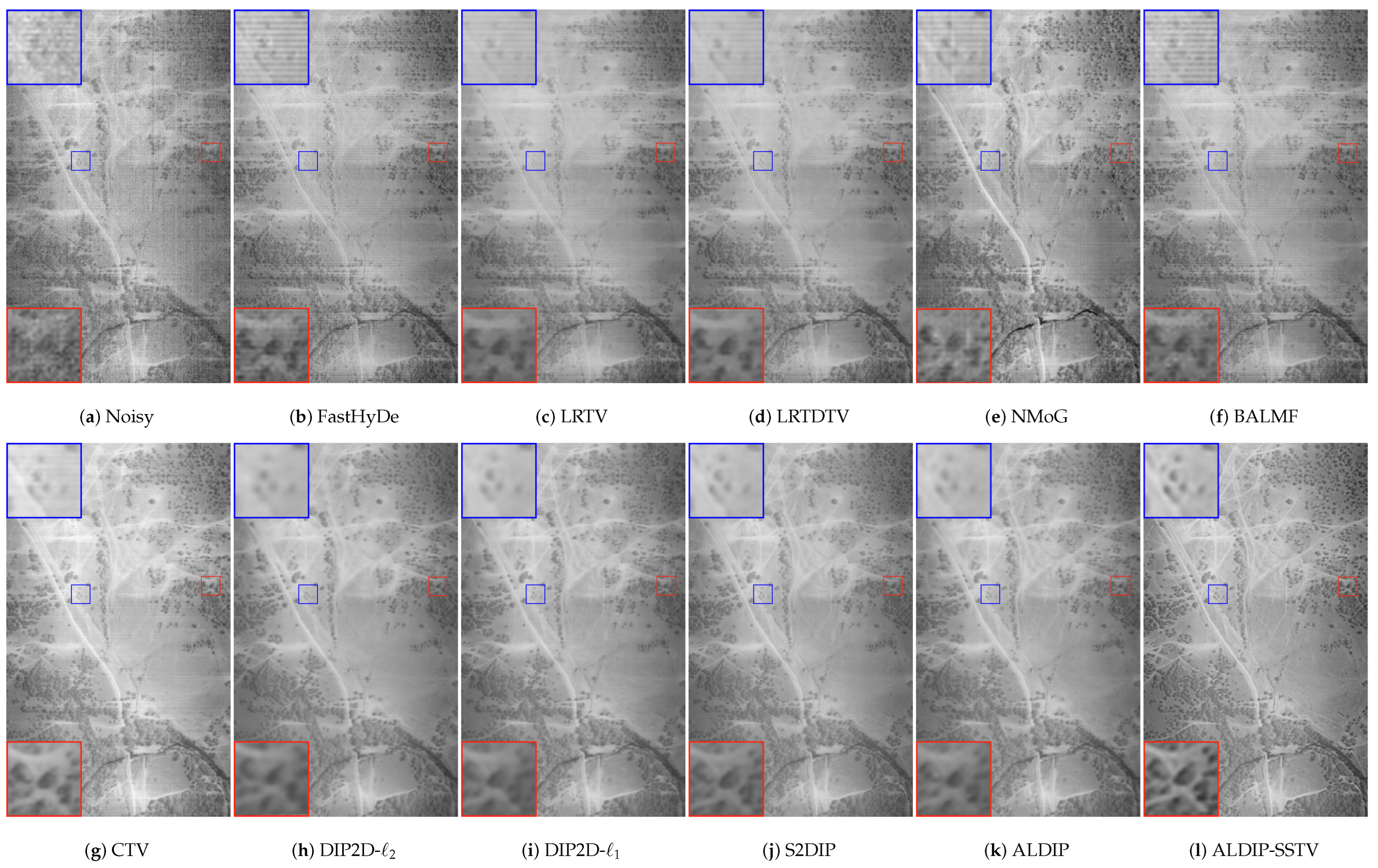
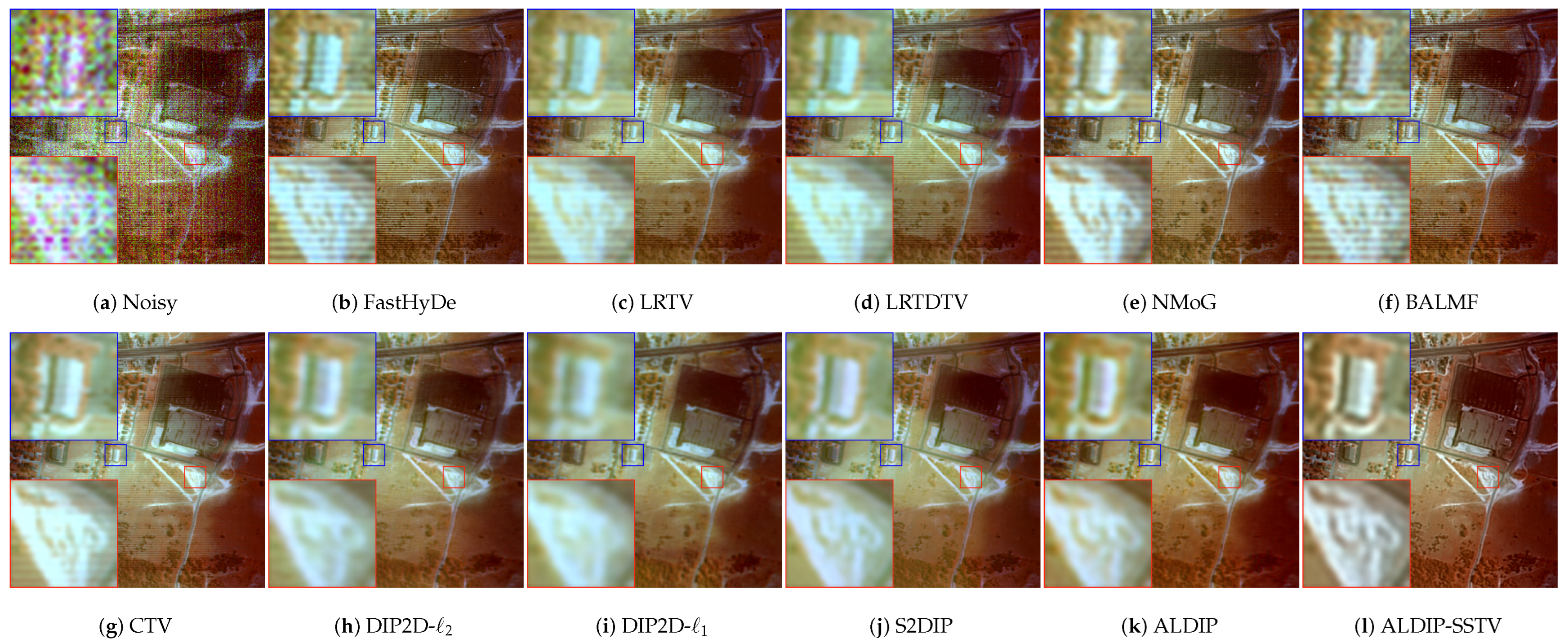
The denoising result of the Terrain dataset is shown in Figure 9. Apparently, all non-DIP-based methods cannot completely remove stripes. Among the DIP-based methods, the results of ALDIP and ALDIP-SSTV are less blurring and preserve more details. On the Urban dataset, the effectiveness of our methods is more significant. As shown in Figure 10, non-DIP-based methods have poor performance. It can be seen visually that ALDIP and ALDIP-SSTV outperform all other methods.

Figure 9. Noisy and denoising results by methods for comparison on real-world noisy HSI Terrain dataset. The images of band 104 are displayed. Two local areas (red and blue squares) are demarcated zoomed for easy observation.

Figure 10. Noisy and denoising result by methods for comparison on real-world noisy HSI Urban dataset. The pseudo images consisted of the 104th, 108th and 109th bands are displayed. Two local areas (red and blue squares) are demarcated zoomed for easy observation.

4.3. Sensitivity Analysis

At the first glance, ALDIP needs to initialize parameters $\lambda$ and $\kappa$. Let us revisit Equation (22), and it is shown that only $\kappa$ should be initialized, because updating $\lambda$ depends on $\kappa$ rather than the previous $\lambda$. In practice, we do not know whether the noise is negative skew, positive skew or symmetric. An intuitive strategy is to initialize ${\kappa }_k=(k=1,2,\cdots ,B)$, which corresponds to the symmetric case.

As stated before, the loss function of ALDIP can actually be deemed as the weighted ${\ell }_1$ norm, where the weight is determined by $\lambda$ and $\kappa$. DIP2D-${\ell }_1$ is hence employed as the baseline. Figure 11 exhibits the PSNR curve versus a different initial value of $\kappa$. It is revealed that the PSNR of ALDIP fluctuates within a very small interval and is always higher than that of the baseline. A conclusion is thus drawn that ALDIP is not sensitive to the initial value of $\kappa$.

Figure 11. The trend of PSNR changing with the initial value of $\kappa$ on Indian Pines (case 8) and Pavia Centre (case 12).

Furthermore, as shown in Figure 12, it is found that ALDIP can always reach the optimal PSNR value with fewer iterations than DIP2D-${\ell }_1$, no matter how $\kappa$ is initialized. This indicates that DIP guided by AL noise modeling has a faster learning process.

Figure 12. The trend of iterations to reach the best PSNR changing with the initial value of $\kappa$ on Indian Pines (case 8) and Pavia Centre (case 12).

DIP-based methods require early stopping to avoid the inherited overfitting issue. Therefore, the number of steps is a critical hyperparameter that affects the performance of our methods. Figure 13 visualized how the number of steps impacts the performance of our methods. As shown in Figure 13, the PSNR values on both the Indian Pines and Pavia Centre datasets approach their respective peaks at around 800 iterations when the image suffers from i.i.d. Gaussian noise (case 1). There is a similar conclusion for non-i.i.d. Gaussian noise (case 2). For the mixed noise, cases 5, 8 and 10 are selected to be displayed. At about 1500 iterations, ALDIP reaches a high PSNR value on both datasets. Thus, we set the number of steps to 800 for Gaussian noise cases and 1500 for the mixed noise cases.

Figure 13. The empirical number of steps for experiments and how different numbers of steps impact the noise removal results.

4.4. Execution Time

Table 5 presents the execution time and corresponding PSNR of DIP-based methods when achieving their optimal PSNR. It is shown that although DIP2D-$l_2$ has the shortest execution time, its performance is far inferior to other methods. Among DIP2D-$l_1$, S2DIP and ALDIP, ALDIP exhibits the shortest execution time and the best performance. Although we need to update the parameters of AL at each iteration, it is not a time-consuming process. Even with the additional time required for updating the parameters of AL, ALDIP still exhibits a shorter execution time due to improvements in learning speed. Under the guidance of AL noise modeling, DIP is accelerated significantly. However, incorporated with the SSTV term, ALDIP-SSTV has the longest execution time. This is because the backpropagation process of the SSTV term is time-consuming.

Table 5. The execution time (Exe. time) and PSNR of DIP-based methods on Indian Pines (case 8) and Pavia Centre (case 12).

Datasets	Metrics	DIP2D-${\mathit{\ell }}_2$	DIP2D-${\mathit{\ell }}_1$	S2DIP	ALDIP	ALDIP-SSTV
Indian Pines	Exe. time	72.29	123.74	341.27	114.23	660.58
	PSNR	29.27	45.75	46.61	47.44	50.00
Pavia Centre	Exe. time	42.75	109.48	128.90	74.59	231.91
	PSNR	32.03	44.91	44.95	45.74	46.46

5. Conclusions

In this paper, considering the asymmetric and heavy-tailed properties of HSI noise, we combine an AL noise model and deep image prior. We propose ALDIP and ALDIP-SSTV for HSI denoising. Compared with other state-of-the-art methods, our methods outperform other methods for both synthetic data and real-world data. As unsupervised-learning-based methods, ALDIP and ALDIP-SSTV avoid training on massive paired data. There are still several directions to further improve our methods. For instance, it is still urgent to design the automatic early stopping strategy to replace manual monitoring. Moreover, except for SSTV, other more advanced regularizations can be combined into ALDIP. Last but not least, the construction of a more suitable network architecture for HSI denoising is also an interesting problem. Additionally, our methods focus on modifying the loss function to enable the network to learn the asymmetric and heavy-tailed properties of complex noise. It would be interesting to design a learnable module that can achieve the same objective in the future.