Abstract
Recently, self-supervised multi-view stereo (MVS) methods, which are dependent primarily on optimizing networks using photometric consistency, have made clear progress. However, the difference in lighting between different views and reflective objects in the scene can make photometric consistency unreliable. To address this issue, a geometric prior-guided multi-view stereo (GP-MVS) for self-supervised learning is proposed, which exploits the geometric prior from the input data to obtain high-quality depth pseudo-labels. Specifically, two types of pseudo-labels for self-supervised MVS are proposed, based on the structure-from-motion (SfM) and traditional MVS methods. One converts the sparse points of SfM into sparse depth maps and combines the depth maps with spatial smoothness constraints to obtain a sparse prior loss. The other generates initial depth maps for semi-dense depth pseudo-labels using the traditional MVS, and applies a geometric consistency check to filter the wrong depth in the initial depth maps. We conducted extensive experiments on the DTU and Tanks and Temples datasets, which demonstrate that our method achieves state-of-the-art performance compared to existing unsupervised/self-supervised approaches, and even performs on par with traditional and supervised approaches.
1. Introduction
Multi-view stereo (MVS) aims to generate a 3D model of a scene using a set of images with known poses, which has various applications in augmented reality, virtual reality, robotics, remote sensing, and more [1,2]. In the past years, the traditional MVS methods, such as MVE [3], OpenMVS [4], and COLMAP [5,6] have developed rapidly. Recently, the introduction of deep learning has allowed supervised MVS methods to outperform these traditional methods. Benefiting from the powerful feature representation ability, the learning-based MVS methods can efficiently reconstruct more complete 3D scenes [7]. Learning-based methods, however, require a significant quantity of large-scale 3D labeled data for training. This is difficult to obtain due to the challenges associated with creating 3D annotations [8,9], which generally involve capturing multiple synchronized images and depth sensors.
To solve the dependence on 3D annotated data, several unsupervised/self-supervised methods have been proposed [10,11,12,13,14]. These methods generally use the photometric consistency loss as the main loss, which measures the color consistency of original images and reconstructed images, based on estimated depth maps. In essence, it is assumed that the objects satisfy photometric consistency in different perspectives, that is, the projection of identical 3D scene points on different views conforms to color consistency. However, in the real world, due to the different lighting conditions from different perspectives and the reflection and occlusion problems in some areas, the assumption of photometric consistency sometimes does not hold. As a result, the photometric consistency loss is not always reliable. To this end, some self-supervised MVS methods, which [14,15] leverage pseudo-labels to solve the ambiguity of photometric consistency loss, have been proposed. These methods [14,15] usually adopt a two-stage training strategy. First, the network is primarily trained based on photometric consistency loss, resulting in the generation of an initial depth map; second, the pseudo-labels are generated by refining the initial depth map.
Although self-supervised methods based on pseudo-labels have achieved comparable performance to supervised methods, the process of generating pseudo-labels is very cumbersome and time-consuming, which is not conducive to practical application. To address this issue, we propose the geometric prior-guided multi-view stereo (GP-MVS) approach for self-supervised learning. The GP-MVS method uses geometry priors to efficiently generate high-quality depth pseudo-labels for self-supervised MVS. Specifically, we propose two types of depth pseudo-labels, sparse and semi-dense, based on the geometry information of the 3D scene. For the sparse labels, we use structure-from-motion (SfM) [5] to obtain sparse points, and convert them into depth maps as pseudo-labels. We add spatial smoothness constraints as supervision with the sparse labels to improve performance. For the semi-dense labels, we employ the traditional MVS method COLMAP [6] to produce the initial depth maps. We then apply geometric consistency constraints to remove outliers from these maps. As a result, we obtain high-quality pseudo-labels by combining the geometric priors, which can effectively avoid mis-estimation due to unreliable photometric consistency. From the experimental results, we can see that our method demonstrates exceptional performance when compared to other self-supervised methods, and is even comparable with some of the top supervised methods.
The key contributions of this work are as follows:
- (1)
- An efficient geometric prior-guided self-supervised learning framework for MVS is proposed.
- (2)
- A sparse prior loss, that combines sparse depth pseudo-labels from the SfM and the spatial smoothness constraint, is introduced, to better deal with depth discontinuities under sparse supervision.
- (3)
- A semi-dense depth pseudo-label from the initial depth map estimated by COLMAP and geometric consistency is applied, to remove outliers caused by unreliable photometric consistency.
2. Related Work
2.1. Traditional MVS
Traditional MVS methods are able to be categorized into three groups according to how they represent the 3D scene: point cloud-based [16,17], volumetric-based [18], and depth map-based methods [6,19,20,21,22,23,24,25]. The first class of methods usually adopts the propagation strategy for matched keypoints, to gradually densify the reconstruction. However, due to the sequential propagation strategy, these methods are difficult to parallelize. The second class of methods represents the 3D space as regular voxels and determines the proximity of each voxel to the surface. These methods usually have high memory consumption, due to the voxel representation. The third class of methods separates the problem into a depth map estimation and depth map fusion, which are easy to parallelize and convert to a point cloud representation.
Depth map-based MVS methods can be implemented using various software packages, such as Multi-View Environment (MVE) [3], which offers end-to-end reconstruction capabilities including SfM, MVS, surface reconstruction, and texturing. Gipuma [21], COLMAP [6], ACMM [23], DP-MVS [24], and PatchMatch MVS [25] are PatchMatch-based [26] MVS methods. COLMAP employs geometric priors and photometric consistency to estimate surface normals and depth maps. ACMH [23] introduces an adaptive checkerboard sampling strategy to improve the efficiency of the PatchMatch-based method, ACMM further uses multi-scale geometric consistency based on ACMH, to improve the robustness of the method. In this paper, we adopt the widely used COLMAP to generate pseudo-labels.
2.2. Learning-Based MVS
Learning-based MVS methods have recently begun to shown great potential. MVSNet [27] presented an end-to-end pipeline, which estimated depth by building a 3D cost volume and using 3D CNN to regularize and regress the initial depth map. Following this, most learning-based methods [28,29,30] have mainly followed the pipeline of MVSNet. Some methods [31,32,33] leverage the RNN to regularize the cost volume sequentially, reducing memory overhead while increasing inference time. To both reduce time and memory consumption, the authors in [1,34,35,36] adopt the coarse-to-fine strategy. They estimate coarse estimates first and then make accurate estimates based on the previous stage’s results. These methods achieve high-accuracy and high-resolution estimates, with acceptable memory and time cost. Based on the coarse-to-fine architecture, MVSFormer [37] introduced the pretrained ViT enhanced multi-view feature extraction network, which can learn more reliable feature representations, benefiting from informative priors from ViT. In this paper, CasMVSNet [35] is used as the backbone.
Supervised learning methods rely on hard-to-obtain 3D annotations. Thus, researchers began to focus on unsupervised/self-supervised methods [10,11,12,13,14]. UnsupMVS [10] was the first learning-based network that solved the MVS problem without ground-truth training data, which relies on the photometric consistency between multiple views. [11] adopts the geometric consistency between multiple views. [12] extracts features with more semantic information by using a pretrained VGG network, and optimizes the initial depth map with normal–depth consistency. JDACS [13] introduces a self-supervised MVS framework based on co-segmentation and data-augmentation. Self-sup CVP-MVSNet [14] uses a two-stage training strategy, where the initial depth maps are estimated based on photometric consistency, followed by depth map refinement from high-resolution images and neighboring views. U-MVS [15] uses the correspondence information provided by optical flows and uncertainty maps to handle wrong supervision in the foreground and background, respectively. These methods heavily depend on photometric consistency, that is ambiguous in real 3D scenes. To overcome this, we consider leveraging traditional methods to generate pseudo-labels for self-learning.
3. Method
Our objective is to produce accurate and reliable pseudo-labels to facilitate self-supervised learning of MVS. In this section, we first analyze the wrong supervision caused by photometric consistency loss, then we present the two proposed kinds of pseudo-labels. The first type is sparse pseudo-labels, which are obtained by generating sparse points from SfM and then converting them into sparse depth maps. The second type is semi-dense pseudo-labels, which are generated using the traditional MVS method to estimate initial depth maps, followed by filtering out the outliers using geometric consistency.
The overall geometric prior-guided self-supervised learning framework is depicted in Figure 1. At the top of the figure, are the two pseudo-labels proposed for network training, which will be given in Section 3.2 and Section 3.3. The bottom part shows a sketch of a learning-based MVS network.
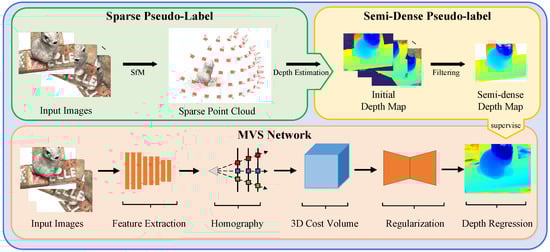
Figure 1.
Geometric prior-guided self-supervised learning MVS framework. We generate the sparse and semi-dense pseudo-labels by using SfM and the traditional MVS method. These labels are then used to supervise the training of our MVS network.
3.1. Photometric Consistency Loss Revisited
The photometric consistency loss, , measures the resemblance between the source image, , projected to the reference view, according to the estimated depth maps and the reference image, :
where ▽ represents the gradient, and is the effective area of the image.
Although the photometric consistency loss between different views can serve as supervision for self-supervised learning, there are still two issues that remain unresolved. (1) As shown in Figure 2, in a real scene, there is often interference from reflective surfaces, object occlusion, or other factors, and the corresponding points in different perspectives do not always meet the conditions of photometric consistency; (2) the supervision of the background areas in the DTU dataset is invalid. Specifically, there are invisible areas between different views, thus, the reconstructed image, , usually contains invalid areas, and using photometric consistency loss will introduce large errors.
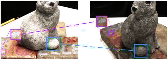
Figure 2.
Ambiguity when adopting photometric consistency.
To solve these issues, we propose two pseudo-labels as supervision. In Figure 1, the sparse pseudo-label is located in the top left, while the semi-dense pseudo-label can be found in the top right. The pseudo-label-based self-supervised MVS framework can learn 3D information well and efficiently, even under reflective surfaces, object occlusion, and illumination changes.
3.2. Sparse Pseudo-Label
This section covers the generation of sparse depth map pseudo-labels. SfM [5], as a pre-step for MVS, aims to predict camera parameters of input images and 3D sparse point clouds of the scene. By triangulating feature points that match across multiple images, a set of sparse 3D points is obtained. These points are then optimized through bundle adjustment and outlier filtering, ensuring that the remaining sparse points are sufficiently reliable. Figure 3 shows the generation of sparse pseudo-labels, where only the white points in the depth map contain sparse prior information. Specifically, we generate sparse pseudo-labels based on the sparse point clouds , and the camera parameters from SfM. For visible sparse point in view i, we transform the world coordinates into camera coordinates , with the extrinsic :
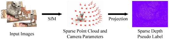
Figure 3.
Generation of sparse pseudo-label.
Then, we project the sparse 3D points (camera coordinates) to the 2D image. For point in a sparse point cloud, we get the projected point , with the intrinsics:
where and from are the pixel focal length and the principal point, respectively. z denotes the depth d of . For those points without prior depth values, we set their depth as 0.
The sparse depth map only provides supervision for some pixels in the estimate. Therefore, we add the depth smoothing loss. The aims of the depth smoothing loss are to make the gradient of the estimate change smoothly and allow discontinuities in depth with large color changes. The depth smoothing loss considers variations in gradients of the input image:
where p is the pixel in the depth map and the image , and is the gradient of the estimate. Thus, the sparse prior loss that we adopt when training the network is:
where represents the loss between the sparse pseudo-label and estimate. is the weight parameters of the two losses in our training with a sparse pseudo-label, is empirically set to 0.1 [13]. is the weight coefficient of the in different stages.
3.3. Semi-Dense Pseudo-Label
The sparse pseudo-label can only provide supervision for a few points in the estimated depth maps, which can constrain the network’s learning capability. Therefore, we consider generating a pseudo-label based on the traditional MVS method, to obtain more dense pseudo-labels. COLMAP [6] is a widely used method for 3D reconstruction, which performs pixel-wise normal and depth estimation based on geometric and photometric consistency. However, for weak textures and background areas, the reconstruction results of COLMAP are generally not reliable, this is due to the ambiguity of photometric consistency. To ensure the production of dependable pseudo-labels for self-supervised learning, we initially employ COLMAP to generate a preliminary depth map and then utilize multi-view geometric consistency to eliminate any outliers.
The initial depth map produced by COLMAP undergoes a filtering process that involves checking for geometric consistency through depth reprojection error, as shown in Figure 4. To be specific, the image i and j are related by their relative position represented by the matrix . The estimated depth of point p in the reference view is denoted as . Back-projecting the point p into 3D space based on , is obtained. Projecting to the source image, gives the projected pixel q of the source view. Back-projecting the q in the source image based on its depth estimate to 3D space, gives the point . Projecting to the reference image gives the projected pixel coordinates . The coordinate reprojection error is expressed as . Similarly, the relative depth reprojection error is expressed as .
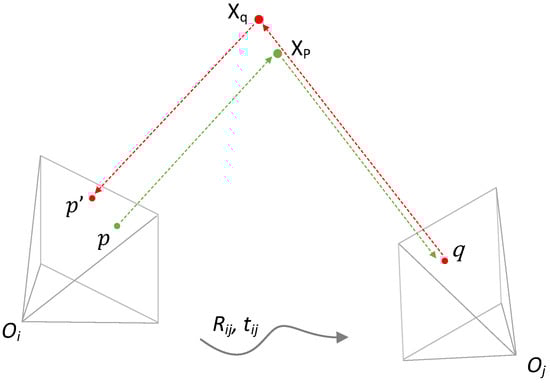
Figure 4.
Cross-view geometric consistency.
We define a criterion to determine whether the estimated depth of pixel p satisfies the cross-view geometric consistency, which comprehensively considers the coordinate reprojection error and relative depth reprojection error of the depth map. We consider the to be consistent between the two views if the following equation is satisfied:
where and are empirically set to 1 and 0.01 based on the geometric consistency used in the previous method [27].
The initial depth map, estimated based on the traditional geometric method, is denoted as . For the p in the reference image, there are source images for the multi-view geometric consistency check, and we can obtain pixels reprojected to the reference image. If the reprojected depth values are consistent for at least views, i.e., , then the estimate is considered dependable; represents the minimum number of views necessary to achieve depth consistency. The retained high-confidence depth map is denoted as , which is the semi-dense pseudo-label used for model training.
As shown in Figure 5, after the cross-view geometric consistency check, the erroneous background area in the depth map is filtered basically, while the depth estimation in the foreground part is retained. The multi-view geometric consistency check avoids invalid supervision of the background area, which is more conducive to the training of the network model.
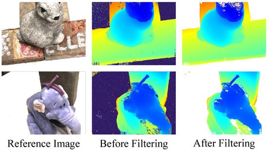
Figure 5.
Semi-dense pseudo-label with cross-view geometric consistency.
We adopt the semi-dense loss when training the network with semi-dense pseudo-labels:
we follow the multi-stage training strategy of the backbone network [35], where is the estimate of stage l, and is the pseudo-label. denotes valid pixels in the pseudo-label. is the weight of the loss items in different stages.
3.4. Geometric Prior-Guided Multi-View Stereo Network
CasMVSNet [35] is used as our baseline model, and we apply the proposed sparse prior loss or semi-dense loss to supervise the network during training. The coarse-to-fine strategy is utilized by CasMVSNet [35] for estimating high-resolution depth maps. It first uses a weight-sharing feature pyramid network [38] to extract multi-scale features () from all input images, with resolution . For each scale, the features are then warped into fronto-parallel planes of the reference view, using differentiable homography [27], to obtain feature volumes. By calculating the variance-based similarity, the feature volumes are combined to construct the 3D cost volume. Subsequently, the raw cost volume is regularized using a 3D UNet, resulting in a pixel-wise depth probability distribution. From this distribution, the is obtained by taking the expectation value. Finally, the depth map , with resolution , can be obtained by gradually decreasing the depth sampling range and the depth sampling number of cost volumes, according to the predictions of previous stages.
4. Experiments
In this section, the performance of the GP-MVS framework is evaluated on the DTU [39] and Tanks and Temples benchmark [40]. We begin by describing these datasets and providing implementation details. Subsequently, we present the benchmarking process carried out on the aforementioned datasets. Finally, an ablation study is presented, to showcase the benefits of utilizing the proposed pseudo-labels.
4.1. Datasets and Implementation Details
4.1.1. Datasets
DTU is a dataset that comprises over 100 indoor scenes captured in a laboratory environment and featuring 7 distinct lighting conditions. Each scene consists of 39 or 64 images. We adopt the sparse prior generation process proposed in Section 3.2, and use the camera projection transformation to obtain the sparse depth map pseudo-labels. For semi-dense depth map pseudo-labels, as presented in Section 3.3, the initial depth maps are generated using COLMAP [5], and then we employ geometric consistency to remove any outliers.
We use metrics of mean accuracy, mean completeness, overall score, and the 0.5 mm F score for this dataset. These metrics are given by Equations (8)–(11), respectively.
where , measures the distance from each point in the reconstructed point cloud to the ground-truth point cloud .
where , measures the distance from each point in the ground truth point cloud to the reconstructed point cloud
where the precision , measures the percentage of the number of reconstructed point clouds that fall within a given distance threshold , to the total number of reconstructed point clouds, the recall , measures the percentage of the number of ground-truth point clouds to the total number of ground-truth point clouds at a given distance threshold . The and are given by Equations (12) and (13), respectively.
Tanks and Temples is a dataset consisting of indoor and outdoor scenes captured in realistic environments, and it includes the intermediate set and the advanced set. Our method is evaluated for its generalization performance using this dataset, with the F score serving as the primary metric.
4.1.2. Implementation Details
Training. We used generated pseudo-labels to supervise the backbone network [35,37] on the training set of DTU. Similar to CasMVSNet [35], the high-resolution input images and pseudo-label depth maps, with resolution 1600 × 1200, were down-sampled and center-cropped to obtain image and depth maps with a resolution of 640 × 512 when training. PyTorch was used to implement the network, and a total of 16 epochs were used to train the network with the Adam optimizer. The initial learning rate of 0.001 was halved at the 10th, 12th, and 14th epochs, to prevent the network training from falling into a local optimum. Following CasMVSNet [35], we employed 48, 32, and 8 hypothesis planes at each stage, and the for each stage was set to 0.5, 1.0, and 2.0.
Depth Fusion. After generating depth maps for all reference views, we fused them to create a dense 3D point cloud model, using a similar approach to previous work [35]. We started by filtering out unreliable depth values with low confidence, using the probability map generated by the network. We then applied the geometric consistency check in Equation (6) to verify the depth maps, further filtering out unreliable depths. The final depth estimation for each pixel was obtained by taking the average over all reprojected depths. Finally, we directly reprojected the filtered depth maps into space to generate the 3D point cloud.
4.2. Benchmark Performance
Results on DTU. Our method’s performance is assessed on the DTU test set using the network trained on the DTU training set. As for the supervised backbone CasMVSNet [35], the resolution of the input is resized to and five images are used for depth map prediction (one reference image and four source images).
We evaluate the point clouds reconstructed by our method using the overall score. As summarized in Figure 6, our approach that utilizes semi-dense depth pseudo-labels delivers performance that is comparable to self-supervised learning approaches and even outperforms the supervised MVSNet [27], R-MVSNet [31], and Point-MVSNet [34], and the result is roughly on par with those of CasMVSNet [35] and CVP-MVSNet [36].
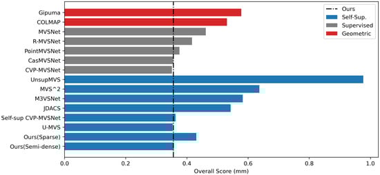
Figure 6.
Comparison between SOTA MVS methods on DTU dataset (lower is better).
The quantitative results of various self-supervised MVS methods, including the proposed pseudo-label based method, are presented in Table 1. Our methods (trained with sparse pseudo-labels or semi-dense pseudo-labels) perform better than UnsupMVS [10], MVS2 [11], M3VSNet [12], and JDACS [13]. The model trained with our semi-dense depth map pseudo-labels (semi-dense) achieved comparable performance compared with Self-sup CVP-MVSNet [14] and U-MVS [15]. Note that the pseudo-labels generation process of Self-sup CVP-MVSNet and U-MVS is much more complicated compared with that of our method. For Self-sup CVP-MVSNet, after obtaining the initial depth map from the unsupervised model, an iterative refinement process is performed to obtain the pseudo-labels, which involves several steps, such as initial depth estimation from a high-resolution image, consistency check-based filtering for estimates, and fusion of the depth from multiple views, to obtain final pseudo-labels. For U-MVS, it uses the pretrained unsupervised model based on the uncertainty to generate pseudo-labels, which requires sampling up to 20 times to obtain reliable uncertainty maps for depth filtering.

Table 1.
Quantitative results of our method against self-supervised MVS methods on the DTU dataset (lower is better). The best results are in bold, while the second ones are underlined.
Table 2 showcases a comparison between the proposed methods and traditional/supervised MVS methods. Our approach surpasses the traditional approaches Gipuma [21] and COLMAP [6]. MVSFormer [37] has been improved on the basis of CasMVSNet [35], achieving the best performance of the supervised methods on the DTU dataset. Our self-supervised method is comparable to the supervised multi-scale MVS network CVP-MVSNet [14], and the point cloud reconstructed by our method has better completeness. We also compare the self-supervised approach proposed with the backbone network CasMVSNet. Table 2 presents a numerical evaluation of our approach compared to the CasMVSNet on the DTU dataset. Our approach shows slightly lower quantitative results but the qualitative results, as shown in Figure 7, suggest that our approach can reconstruct 3D point clouds with high accuracy, especially in capturing local details.
Table 2.
Quantitative results of our approach against traditional and supervised MVS methods on the DTU dataset (lower is better). The best results are in bold, while the second ones are underlined.
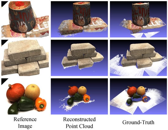
Figure 7.
Qualitative results of our approach on the DTU dataset in terms of reconstructed point clouds.
Results on Tanks and Temples. To assess the generalization capability of the proposed methods, the models were trained on the DTU dataset and performed an evaluation on the Tanks and Temples dataset, without any fine-tuning. Specifically, five input images were used as an input, with a resolution of . As displayed in Table 3, our approach surpasses the traditional methods and supervised methods by a significant margin, which proves that the MVS network supervised with our proposed pseudo-label is effective. Additionally, Figure 8 illustrates the qualitative results of both subsets. The proposed method can reconstruct denser point clouds with more details, making them more visually appealing.
Table 3.
The performance of our approach on the Tanks and Temples benchmark (intermediate set) with F score (%) (higher is better). The best results are in bold, while the second ones are underlined.
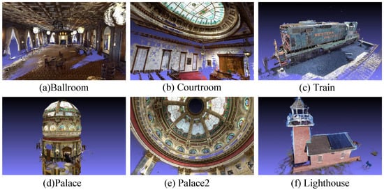
Figure 8.
Visualization of the reconstructed point clouds on the Tanks and Temples dataset.
The advanced set of Tanks and Temples contains challenging scenes. Our approach demonstrates superior performance compared to other approaches in most evaluation metrics, as presented in Table 4. This proves that the proposed depth map pseudo-labels based on the geometry prior, can effectively capture the geometric information in the 3D scene. Due to overfitting on the DTU dataset, supervised methods, such as the backbone CasMVSNet, exhibit limited generalization performance. Thus, even though our method achieved slightly lower reconstruction performance on the DTU compared to the backbone network, the use of our proposed pseudo-labels has the potential to enhance the network’s generalization ability. This proves that the MVS network supervised with our proposed pseudo-labels is effective.
Table 4.
The performance of our approach on the Tanks and Temples benchmark (advanced set) with F score (%) (higher is better). The best results are in bold.
4.3. Ablation Study
Accuracy of pseudo-labels. Figure 9 shows the visualization of different pseudo-labels. The white dots in the sparse depth map are the pixel positions with sparse prior information. The sparse depth map can only describe the basic geometric structure of the 3D scene, focusing more on the rich texture part. The supervision of the semi-dense pseudo-label depth map in the foreground area is more complete. Upon comparison with the ground truth, it can be inferred that the foreground, using semi-dense pseudo-labels, is more complete, while removing false background estimates. We assess the accuracy of the network using various pseudo-labels as supervision on the DTU dataset, with depth prediction accuracy serving as the evaluation metric. In addition, we provide the density (means of percentage of labeled pixels in each image) of different pseudo-labels. Note that the density of the initial depth map without filtering is 100%.
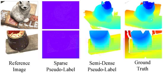
Figure 9.
Visualization of different pseudo-labels.
From Table 5, it can be concluded that the accuracy of the sparse depth map has already achieved a high accuracy (86% pixels of the sparse depth map are accurate within 2 mm). However, due to the few labeled points, the sparse pseudo-labels have certain limitations as supervision. The semi-dense pseudo-labels, after removing the wrong points, has the highest accuracy.
Table 5.
Evaluation of different pseudo-labels. The best results are in bold.
Analysis of Different Supervisions. Table 6 reflects the accuracy of depth maps estimated by models trained under different supervision. The results show that the network trained with semi-dense depth map pseudo-labels achieves the second best accuracy, which is comparable to that of the supervised CasMVSNet, while outperforming the network based on photometric consistency loss and the sparse prior loss.
Table 6.
Qualitative results of depth estimation on the DTU dataset (lower is better). The best results are in bold, while the second ones are underlined.
As shown in Figure 10, using photometric consistency loss as supervision, leads to noticeable errors at the boundaries. In contrast, using semi-dense pseudo-labels as the network’s supervision, allows for more precise depth map predictions, especially at the border between foreground and background.
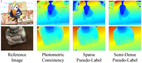
Figure 10.
Quantitative results of depth estimation on the DTU dataset.
Table 7 shows the results of point clouds reconstructed by models with different supervisions. We use the overall and the F score under the 1 mm threshold as the evaluation metrics. Methods based on semi-dense pseudo-labels have the best quality.
Table 7.
Qualitative results of point cloud reconstruction on the DTU dataset (lower is better). The best results are in bold.
By comparing the performance of different methods, we aimed to provide further evidence of the effectiveness of our self-supervised approach utilizing pseudo-labels. Figure 11 displays the reconstructed results of scan9, scan33, and scan49 in the DTU dataset. UnsupMVS [10] is an unsupervised MVS method based on photometric consistency loss. The self-supervised MVS method based on pseudo-labels produces denser 3D point clouds with more complete local details compared to other methods, as shown in Figure 11.
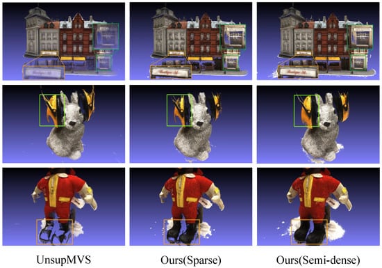
Figure 11.
Quantitative results of point cloud reconstruction on the DTU dataset.
In addition, we conducted a comparison between the point clouds generated by our method and those obtained using traditional methods. The sparse point clouds were generated from the SfM described in Section 3.2. Table 8 demonstrates that although the sparse point cloud has an acceptable accuracy, its completeness is compromised, due to the sparse distribution of points. It should be noted, that our self-supervised methods using semi-dense pseudo-labels outperformed the traditional method COLMAP. In addition, using the dense depth map reconstructed by COLMAP as a pseudo-label for training, the accuracy is not only better than COLMAP itself, but also close to the best supervised learning method, and even stronger in generalization ability. These results highlight the strengths of our proposed pseudo-label approach.
Table 8.
Comparison between traditional methods on the DTU dataset (lower is better). The best results are in bold.
Statistical Analysis. To further show the effectiveness of the proposed semi-dense pseudo-labels, a statistical analysis based on the paired t-test is conducted for CasMVSNet [35] and CasMVSNet [35] combined with semi-dense pseudo-labels. The statistic t of the paired t-test is calculated as:
where denotes the sample mean of differences, denotes the hypothesized population mean difference, denotes the standard deviation of differences, and n denotes the sample size. The degrees of freedom . The p-value is determined by checking the corresponding threshold table based on the t statistic. Table 9 shows the results of the paired t-tests for CasMVSNet [35] and CasMVSNet with our semi-dense pseudo-labels on the DTU dataset and the Tanks and Temples dataset, the significance level is set to 0.05. The p values for the DTU and intermediate subsets are 0.8260 and 0.2794, respectively, indicating no significant difference between the experimental results of CasMVSNet and CasMVSNet with our semi-dense pseudo-labels on these datasets. This suggests that CasMVSNet with our semi-dense pseudo-labels is competitive with CasMVSNet on these datasets. On the advanced subset, the p value is 0.0076, indicating a significant difference between the experimental results of CasMVSNet and CasMVSNet with our semi-dense pseudo-labels on this dataset. Therefore, our method outperforms CasMVSNet significantly on this dataset.
Table 9.
The paired t-test results for CasMVSNet [35] with our semi-dense pseudo-labels on the DTU dataset and the Tanks and Temples dataset (significance level = 0.05).
5. Discussion
Our network’s success can be mainly attributed to the utilization of self-supervised multi-view stereo learning, guided by pseudo-labels. Our pseudo-label-guided method effectively avoids the ambiguity of the breadth of the image reconstruction loss monitoring signal, resulting in a trained network model with stronger generalization performance. However, our work also has some limitations. For instance, the sparse depth supervised network model can only describe the basic structure of the scene, due to insufficient monitoring signals. Additionally, the depth map output from the network model based on sparse prior depth map supervision may not accurately estimate finer details. While using semi-dense pseudo-labels as a supervisory signal can achieve better performance than using sparse pseudo-labels, it is limited by the inherent difficulties of traditional MVS methods in estimating reliable depth in some areas such as occlusion, textureless, and non-Lambertian surfaces, where it cannot provide a supervisory signal for the network.
6. Conclusions
In this paper, a geometric prior-guided MVS framework for self-supervised learning is proposed. Unlike other methods that use photometric consistency loss as supervision, we propose two pseudo-labels: sparse depth map and semi-dense depth map. This can effectively address issues arising from illumination changes across images and inadequate supervision in the background area. Specifically, we employed SfM to obtain a sparse 3D point cloud, and produced depth maps using the traditional MVS method. After post-processing, we obtain two high-quality pseudo-labels, namely sparse and semi-dense. By using these pseudo-labels, our approach outperforms self-supervised methods and performs similarly to supervised learning frameworks. The sparse point cloud mentioned in this paper is low-level information, which only contains geometric information of the 3D scene, while the input image contains more semantic information. Our future work will consider how to combine an image’s semantic information to assist MVS.
Author Contributions
Methodology, F.Z., Y.Q. and L.L.; software, F.Z. and Y.Q.; validation, F.Z., W.S. and Y.Q.; writing—original draft preparation, F.Z. and Y.Q.; writing—review and editing, W.S. and L.L.; visualization, F.Z. and Y.Q.; supervision, L.L. and W.T.; funding acquisition, L.L. and W.T. All authors have read and agreed to the published version of the manuscript.
Funding
This work was supported in part by the National Natural Science Foundation of China (grants 61976227 and 62176096) and in part by the Natural Science Foundation of Hubei Province under grant 2020CFA025.
Data Availability Statement
The DTU dataset can be accessed at https://roboimagedata.compute.dtu.dk/ (accessed on 23 April 2016), and the Tanks and Temples benchmark can be accessed at https://www.tanksandtemples.org/ (accessed on 20 July 2017).
Conflicts of Interest
The authors declare no conflict of interest.
References
- Cheng, S.; Xu, Z.; Zhu, S.; Li, Z.; Li, L.E.; Ramamoorthi, R.; Su, H. Deep stereo using adaptive thin volume representation with uncertainty awareness. In Proceedings of the IEEE/CVF Conference on Computer Vision and Pattern Recognition, Seattle, WA, USA, 13–19 June 2020; pp. 2524–2534. [Google Scholar]
- Gonçalves, G.; Gonçalves, D.; Gómez-Gutiérrez, Á.; Andriolo, U.; Pérez-Alvárez, J.A. 3D reconstruction of coastal cliffs from fixed-wing and multi-rotor uas: Impact of sfm-mvs processing parameters, image redundancy and acquisition geometry. Remote Sens. 2021, 13, 1222. [Google Scholar] [CrossRef]
- Fuhrmann, S.; Langguth, F.; Moehrle, N.; Waechter, M.; Goesele, M. MVE—An image-based reconstruction environment. Comput. Graph. 2015, 53, 44–53. [Google Scholar] [CrossRef]
- Cernea, D. OpenMVS: Multi-View Stereo Reconstruction Library. 2020, Volume 5, p. 7. Available online: https://cdcseacave.github.io/openMVS (accessed on 20 May 2015).
- Schonberger, J.L.; Frahm, J.M. Structure-from-motion revisited. In Proceedings of the IEEE Conference on Computer Vision and Pattern Recognition, Las Vegas, NV, USA, 27–30 June 2016; pp. 4104–4113. [Google Scholar]
- Schönberger, J.L.; Zheng, E.; Frahm, J.M.; Pollefeys, M. Pixelwise view selection for unstructured multi-view stereo. In Proceedings of the European Conference on Computer Vision, Amsterdam, The Netherlands, 11–14 October 2016; pp. 501–518. [Google Scholar]
- Ji, M.; Gall, J.; Zheng, H.; Liu, Y.; Fang, L. Surfacenet: An end-to-end 3d neural network for multiview stereopsis. In Proceedings of the IEEE International Conference on Computer Vision, Venice, Italy, 22–29 October 2017; pp. 2307–2315. [Google Scholar]
- Zhong, Y.; Li, H.; Dai, Y. Open-world stereo video matching with deep rnn. In Proceedings of the European Conference on Computer Vision (ECCV), Munich, Germany, 8–14 September 2018; pp. 101–116. [Google Scholar]
- Zhang, X.; Zhao, Y.; Wang, H.; Zhai, H.; Sun, H.; Zheng, N. End-to-end learning of self-rectification and self-supervised disparity prediction for stereo vision. Neurocomputing 2022, 494, 308–319. [Google Scholar] [CrossRef]
- Khot, T.; Agrawal, S.; Tulsiani, S.; Mertz, C.; Lucey, S.; Hebert, M. Learning unsupervised multi-view stereopsis via robust photometric consistency. arXiv 2019, arXiv:1905.02706. [Google Scholar]
- Dai, Y.; Zhu, Z.; Rao, Z.; Li, B. Mvs2: Deep unsupervised multi-view stereo with multi-view symmetry. In Proceedings of the 2019 International Conference on 3D Vision (3DV), Quebec, QC, Canada, 16–19 September 2019; IEEE: Piscataway, NJ, USA, 2019; pp. 1–8. [Google Scholar]
- Huang, B.; Yi, H.; Huang, C.; He, Y.; Liu, J.; Liu, X. M3VSNet: Unsupervised multi-metric multi-view stereo network. In Proceedings of the 2021 IEEE International Conference on Image Processing (ICIP), Anchorage, AK, USA, 19–22 September 2021; IEEE: Piscataway, NJ, USA, 2021; pp. 3163–3167. [Google Scholar]
- Xu, H.; Zhou, Z.; Qiao, Y.; Kang, W.; Wu, Q. Self-supervised multi-view stereo via effective co-segmentation and data-augmentation. In Proceedings of the AAAI Conference on Artificial Intelligence, Virtual Event, 2–9 February 2021; Volume 35, pp. 3030–3038. [Google Scholar]
- Yang, J.; Alvarez, J.M.; Liu, M. Self-supervised learning of depth inference for multi-view stereo. In Proceedings of the IEEE/CVF Conference on Computer Vision and Pattern Recognition, Nashville, TN, USA, 20–25 June 2021; pp. 7526–7534. [Google Scholar]
- Xu, H.; Zhou, Z.; Wang, Y.; Kang, W.; Sun, B.; Li, H.; Qiao, Y. Digging into uncertainty in self-supervised multi-view stereo. In Proceedings of the IEEE/CVF International Conference on Computer Vision, Montreal, BC, Canada, 11–17 October 2021; pp. 6078–6087. [Google Scholar]
- Lhuillier, M.; Quan, L. A quasi-dense approach to surface reconstruction from uncalibrated images. IEEE Trans. Pattern Anal. Mach. Intell. 2005, 27, 418–433. [Google Scholar] [CrossRef] [PubMed]
- Furukawa, Y.; Ponce, J. Accurate, dense, and robust multiview stereopsis. IEEE Trans. Pattern Anal. Mach. Intell. 2009, 32, 1362–1376. [Google Scholar] [CrossRef] [PubMed]
- Hane, C.; Zach, C.; Cohen, A.; Angst, R.; Pollefeys, M. Joint 3D scene reconstruction and class segmentation. In Proceedings of the IEEE Conference on Computer Vision and Pattern Recognition, Portland, OR, USA, 23–28 June 2013; pp. 97–104. [Google Scholar]
- Shen, S. Accurate multiple view 3d reconstruction using patch-based stereo for large-scale scenes. IEEE Trans. Image Process. 2013, 22, 1901–1914. [Google Scholar] [CrossRef] [PubMed]
- Zheng, E.; Dunn, E.; Jojic, V.; Frahm, J.M. Patchmatch based joint view selection and depthmap estimation. In Proceedings of the IEEE Conference on Computer Vision and Pattern Recognition, Columbus, OH, USA, 23–28 June 2014; pp. 1510–1517. [Google Scholar]
- Galliani, S.; Lasinger, K.; Schindler, K. Massively parallel multiview stereopsis by surface normal diffusion. In Proceedings of the IEEE International Conference on Computer Vision, Santiago, Chile, 7–13 December 2015; pp. 873–881. [Google Scholar]
- Li, Z.; Wang, K.; Meng, D.; Xu, C. Multi-view stereo via depth map fusion: A coordinate decent optimization method. Neurocomputing 2016, 178, 46–61. [Google Scholar] [CrossRef]
- Xu, Q.; Tao, W. Multi-scale geometric consistency guided multi-view stereo. In Proceedings of the IEEE/CVF Conference on Computer Vision and Pattern Recognition, Long Beach, CA, USA, 15–20 June 2019; pp. 5483–5492. [Google Scholar]
- Zhou, L.; Zhang, Z.; Jiang, H.; Sun, H.; Bao, H.; Zhang, G. DP-MVS: Detail Preserving Multi-View Surface Reconstruction of Large-Scale Scenes. Remote Sens. 2021, 13, 4569. [Google Scholar] [CrossRef]
- Stathopoulou, E.K.; Battisti, R.; Cernea, D.; Remondino, F.; Georgopoulos, A. Semantically derived geometric constraints for MVS reconstruction of textureless areas. Remote Sens. 2021, 13, 1053. [Google Scholar] [CrossRef]
- Bleyer, M.; Rhemann, C.; Rother, C. Patchmatch stereo-stereo matching with slanted support windows. In Proceedings of the BMVC, Dundee, UK, 29 August–2 September 2011; Volume 11, pp. 1–11. [Google Scholar]
- Yao, Y.; Luo, Z.; Li, S.; Fang, T.; Quan, L. Mvsnet: Depth inference for unstructured multi-view stereo. In Proceedings of the European Conference on Computer Vision (ECCV), Munich, Germany, 8–14 September 2018; pp. 767–783. [Google Scholar]
- Xue, Y.; Chen, J.; Wan, W.; Huang, Y.; Yu, C.; Li, T.; Bao, J. Mvscrf: Learning multi-view stereo with conditional random fields. In Proceedings of the IEEE/CVF International Conference on Computer Vision, Seoul, Republic of Korea, 27 October–2 November 2019; pp. 4312–4321. [Google Scholar]
- Luo, K.; Guan, T.; Ju, L.; Huang, H.; Luo, Y. P-mvsnet: Learning patch-wise matching confidence aggregation for multi-view stereo. In Proceedings of the IEEE/CVF International Conference on Computer Vision, Seoul, Republic of Korea, 27 October–2 November 2019; pp. 10452–10461. [Google Scholar]
- Xu, Q.; Tao, W. Learning inverse depth regression for multi-view stereo with correlation cost volume. In Proceedings of the AAAI Conference on Artificial Intelligence, New York, NY, USA, 7–12 February 2020; Volume 34, pp. 12508–12515. [Google Scholar]
- Yao, Y.; Luo, Z.; Li, S.; Shen, T.; Fang, T.; Quan, L. Recurrent mvsnet for high-resolution multi-view stereo depth inference. In Proceedings of the IEEE/CVF Conference on Computer Vision and Pattern Recognition, Long Beach, CA, USA, 15–20 June 2019; pp. 5525–5534. [Google Scholar]
- Yan, J.; Wei, Z.; Yi, H.; Ding, M.; Zhang, R.; Chen, Y.; Wang, G.; Tai, Y.W. Dense hybrid recurrent multi-view stereo net with dynamic consistency checking. In Proceedings of the European Conference on Computer Vision, Glasgow, UK, 23–28 August 2020; pp. 674–689. [Google Scholar]
- Wei, Z.; Zhu, Q.; Min, C.; Chen, Y.; Wang, G. Aa-rmvsnet: Adaptive aggregation recurrent multi-view stereo network. In Proceedings of the IEEE/CVF International Conference on Computer Vision, Montreal, BC, Canada, 11–17 October 2021; pp. 6187–6196. [Google Scholar]
- Chen, R.; Han, S.; Xu, J.; Su, H. Point-based multi-view stereo network. In Proceedings of the IEEE/CVF International Conference on Computer Vision, Seoul, Republic of Korea, 27 October–2 November 2019; pp. 1538–1547. [Google Scholar]
- Gu, X.; Fan, Z.; Zhu, S.; Dai, Z.; Tan, F.; Tan, P. Cascade cost volume for high-resolution multi-view stereo and stereo matching. In Proceedings of the IEEE/CVF Conference on Computer Vision and Pattern Recognition, Seattle, WA, USA, 13–19 June 2020; pp. 2495–2504. [Google Scholar]
- Yang, J.; Mao, W.; Alvarez, J.M.; Liu, M. Cost volume pyramid based depth inference for multi-view stereo. In Proceedings of the IEEE/CVF Conference on Computer Vision and Pattern Recognition, Seattle, WA, USA, 13–19 June 2020; pp. 4877–4886. [Google Scholar]
- Cao, C.; Ren, X.; Fu, Y. MVSFormer: Multi-View Stereo by Learning Robust Image Features and Temperature-based Depth. arXiv 2023, arXiv:2208.02541. [Google Scholar]
- Lin, T.Y.; Dollár, P.; Girshick, R.; He, K.; Hariharan, B.; Belongie, S. Feature pyramid networks for object detection. In Proceedings of the IEEE Conference on Computer Vision and Pattern Recognition, Honolulu, HI, USA, 21–26 July 2017; pp. 2117–2125. [Google Scholar]
- Aanæs, H.; Jensen, R.R.; Vogiatzis, G.; Tola, E.; Dahl, A.B. Large-scale data for multiple-view stereopsis. Int. J. Comput. Vis. 2016, 120, 153–168. [Google Scholar] [CrossRef]
- Knapitsch, A.; Park, J.; Zhou, Q.Y.; Koltun, V. Tanks and temples: Benchmarking large-scale scene reconstruction. ACM Trans. Graph. (ToG) 2017, 36, 1–13. [Google Scholar] [CrossRef]
Disclaimer/Publisher’s Note: The statements, opinions and data contained in all publications are solely those of the individual author(s) and contributor(s) and not of MDPI and/or the editor(s). MDPI and/or the editor(s) disclaim responsibility for any injury to people or property resulting from any ideas, methods, instructions or products referred to in the content. |
© 2023 by the authors. Licensee MDPI, Basel, Switzerland. This article is an open access article distributed under the terms and conditions of the Creative Commons Attribution (CC BY) license (https://creativecommons.org/licenses/by/4.0/).