Article

A Random Forest-Based CA-Markov Model to Examine the Dynamics of Land Use/Cover Change Aided with Remote Sensing and GIS

1
Department of Hydrology and Water Resources Management, Institute for Natural Resource Conservation, Kiel University, D-24118 Kiel, Germany
2
Fujian Key Laboratory of Coastal Pollution Prevention and Control, Xiamen University, Xiamen 361102, China
*
Author to whom correspondence should be addressed.
Remote Sens. 2023, 15(8), 2128; https://doi.org/10.3390/rs15082128
Submission received: 31 January 2023 / Revised: 27 March 2023 / Accepted: 11 April 2023 / Published: 18 April 2023

Abstract

:
Understanding the land use/cover change (LUCC) in watersheds is essential for sustainable development. The CA-Markov model has been proven to be an effective method for land use modeling because of its simplicity and potential for evolution. However, it is difficult to apply this method to meet the requirement of land use planning and management since it fails to consider the driving forces of LUCC. To evaluate the factors that influence LUCC comprehensively, we developed and implemented a machine learning-based CA-Markov model to understand the dynamics of LUCC in a coastal watershed in Southeast China, the Minjiang River Watershed (MRW). The proposed method performed well for each land use category, with average AUC values of 0.999 and 0.916 for the training and testing periods, respectively, for suitable images. The overall accuracy for LUCC was 0.971. The urbanization process in the MRW was speeding up recently. Urban area increased by 2.22% of the total area during 2015–2020, and most of that was from conversion of woodland and agricultural land. Additionally, the proposed method provided a much deeper understating of the forces driving the LUCC on a regional scale. Population and gross domestic product (GDP) were the major factors influencing the distribution of urbanized land in the MRW. In contrast, woodland distribution was highly related to topographic factors in the MRW. Scenario analysis was also employed to identify patterns of LUCC under different scenarios. The results showed that the process of urbanization may become more complex with increasing population and GDP and that land use evolution may be more sustainable with scientific spatial plans which consider facilities for people and ecological protection. The proposed method quantifies the LUCC in changing environmental settings and can serve as a helpful tool for sustainable watershed management.

1. Introduction

Land use/cover change (LUCC), as the most direct indicator depicting the effects of human activities on the natural ecosystem, plays a significant role in global change [1,2]. As a complex system constructed by the interaction between natural processes and human activities, regional LUCC is influenced by social, political, and natural factors [3,4,5]. Therefore, assessing and quantifying LUCC patterns is critical for developing regional environmental management and enhancing understanding of the interactions between ecosystems and human activities [6,7,8].
LUCC Modeling has recently attracted considerable interest because LUCC is a complex issue involving physical, environmental, and socio-economic factors [9,10]. Models are one of the most effective tools for understanding the dynamics of LUCC and providing scientific references for rational decision-making [11,12,13]. Therefore, several models have been developed to simulate LUCC patterns. These include the cellular automata Markov chain (CA-Markov) [14], multi-agent models [2], and the logistic regression method [15]. These models have been widely applied to understand land use evolution and play a significant role in spatial planning [9,12]. However, it is still difficult to meet the requirements of land use planning and management with these models because the models lack consideration of the impacts of socio-economic and natural factors [10]. Coupled models were developed recently to comprehend the LUCC on a regional or global scale [10,16].
Coupled with other modeling techniques, the CA-Markov model has greater advantages for simulating changes in complex land use systems through improved accuracy and effective simulation [5,13,17]. Typically, researchers have attempted to assign a suitability score for each factor affecting land use based on experience, a literature review, or the fuzzy-logic method and then quantify the impacts of factors on land use by converting original values to a unified scale, namely, the degree of suitability. After scoring the suitability of each factor, transition rules can be constructed and applied to land use modeling [13]. Fuzzy-logic-based methods, such as logistic regression, have been widely used to build suitability data for land use modeling [13,16,18]. For example, to evaluate urban growth in mountainous cities of Oman, the analytic hierarchy process method was integrated with the CA-Markov model and suggested that urban expansion was initially associated with increased immigration to the urban centers [19]. Additionally, to understand the driving forces of land use, the CA-Markov was integrated with logistic regression models to simulate the law of land use evolution scientifically and suggested that natural and human factors have a major impact on LUCC whereas proximity factors have a relatively small impact [17]. Thus, the CA-Markov model is more scientific and practical than other models [12,20].
Several studies have proven that the uncertainties of the CA-Markov model can be mitigated by considering the driving factors using hybrid methods and assigning suitability scores [9,21]. However, a common problem with the existing methods is that the assigned scores may not reflect land use changes in specific regions [13,22]. For example, fuzzy logic-based methods may produce overfitted models because their rules are based on heuristics, although they can model uncertainty in real world data with continuous boundaries [22,23]. Moreover, these traditional methods may not work well when modeling complex nonlinear relationships between potential driving factors and land use, and the effects of heterogeneity may be discarded or not fully captured, especially for the process of urban development [10,20,24]. Some traditional methods have the limitation of being black-box models, and the statistical significance of the drivers for LUCC is obscured, which may not be conducive to watershed management [10,22]. Thus, it is necessary to minimize these weaknesses when developing a model for land use management [2,10].
Recently, machine learning methods have attracted the attention of geospatial science researchers and have been applied to analyses of remote sensing data [10,17,24]. As a subfield of artificial intelligence, machine learning can overcome the limitations of previous methods and achieve superior or at least equivalent accuracy outcomes [24,25]. Several studies have used machine-learning models to understand land use change in cities or metropolitan regions. For example, by coupling a machine learning method, the evolution of urban space in Shanghai from 2015 to 2030 was simulated under different scenarios and showed that urban development will be more sustainable under the constraints of ecological and cultivated protection [10]. Similarly, the land use/cove in Attica was analyzed based on a machine learning modeling approach and suggested that the high economic growth in Greece may increase built-up area surfaces in this region, accompanied by reductions in natural areas and croplands [26]. However, most related studies have focused on the evolution of urbanization, and these methods have rarely been introduced to evaluate multiple land use types at global or regional scales. The random forest (RF) algorithm, one of the most important machine learning methods, can function as a “white box” method because of its better interpretability for analyzing the contributions of spatial variables [17,26].
Land use modeling has been developed as an important tool for analyzing LUCC dynamics for policy and strategy development, particularly in rapid developing countries [9,10], and RF has proven to be a suitable machine learning algorithm with good interpretability and moderate time complexity [10]. However, few studies have combined machine learning models with the CA-Markov model, and limited regional scale research has been conducted in China. To close these knowledge gaps, the major aim of this study was to integrate the CA-Markov model with the RF algorithm to understand the dynamics in LUCC under specific scenarios. To identify the impacts of multiple variables on land use evaluation at the regional scale, we applied this coupled model to the largest watershed in Southeast China, namely, the Minjiang River Watershed (MRW), which is under increasing pressure from continuous population growth, rapid socio-economic development, and limited natural resources. The objectives of this study were to (1) quantify the land use change in Southeast China, (2) analyze the evolution of land use under different scenarios, and (3) understand the role of strategic spatial planning in regional land use change and provide in-depth implications for sustainable watershed management.

2. Material and Methods
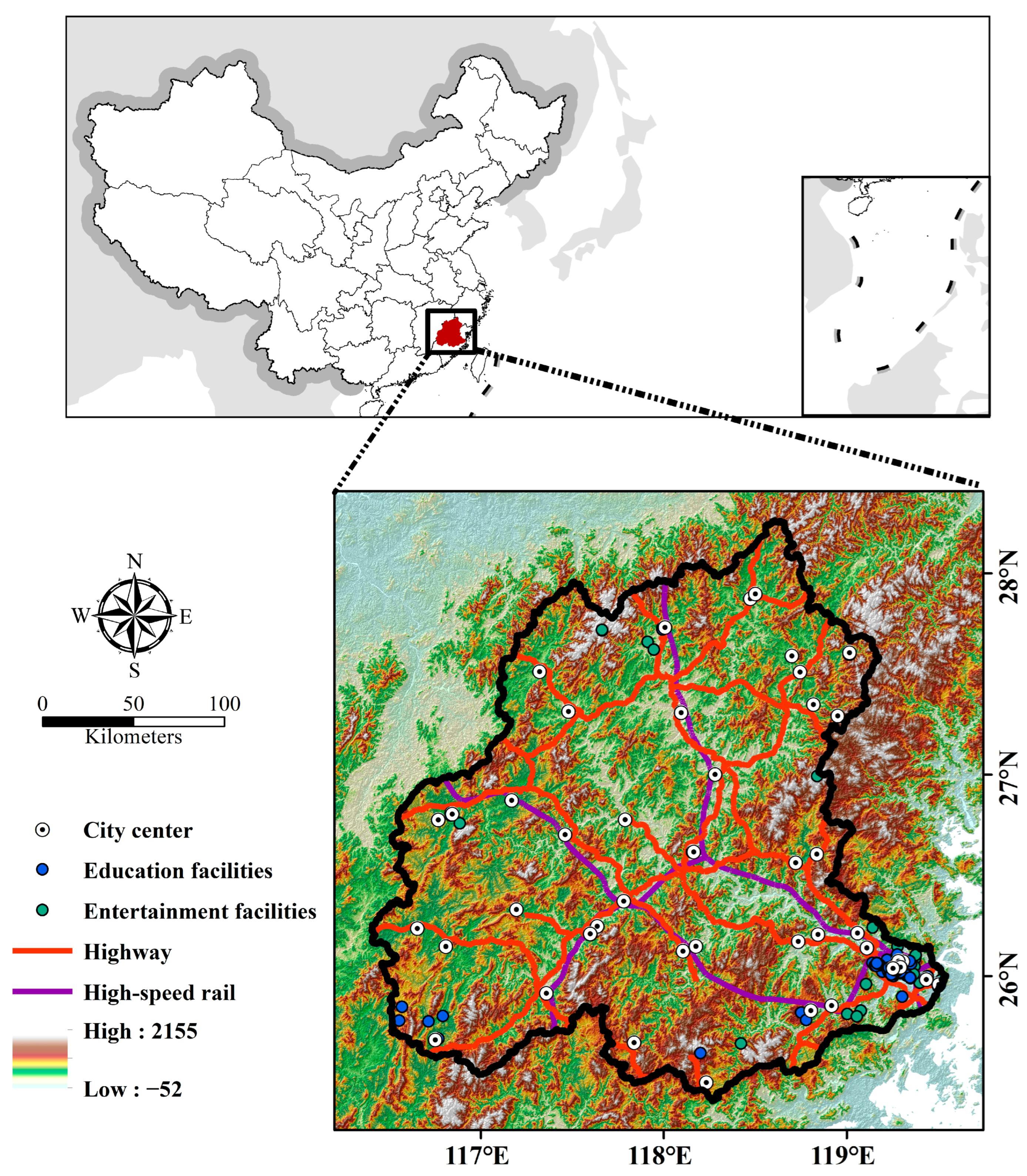
2.1. Study Area

With an area of 60,992 km2, the MRW (25°23′–28°19′ N, 116°23′–119°43′ E) is the largest watershed in Southeast China. Located in the subtropical zone, the MRW has a mean annual temperature and precipitation of 18 °C and 1617 mm, respectively, and approximately 70% of the precipitation occurs between April and September [27,28]. Based on official population records, the populations in 2010, 2015, and 2020 were 10.75, 11.02, and 11.72 million, respectively. More than 60% of the population lives in urban areas (Figure S1). The gross domestic product (GDP) increased by approximately 200% in the past 10 years, from 417 billion CNY (2010) to 1292 billion CNY (2020) (Figure S1). By 2021, more than 1900 km of high-speed railway and 6000 km of highways had been built in Fujian Province, and 60% of this is within the MRW. Additional highways and high-speed railways are planned to be constructed by 2030, which may change the land use patterns in the MRW (Figure 1).

2.2. Data Sources

Following the completion of the first high-speed line in 2009, anthropogenic activities in the MRW increased significantly from 2010. Thus, Landsat images of the MRW were obtained from the USGS Earth Explorer (https://earthexplorer.usgs.gov/, accessed on 17 January 2022 for the years 2010, 2015, and 2020. After examining the available images, we realized that the uncertainties caused by clouds were more significant than those induced by inconsistent dates. Therefore, different dates were used to obtain complete and cloud-free coverage of the study area (Table 1). The unsupervised classification of the Landsat images was performed using the Iterative Self Organizing Data Analysis Technique Algorithm (ISODATA) integrated with post-classification enhancement [29,30]. This method has been proven effective for understanding LUCC [30,31]. Ancillary data, including high-resolution images from Google Earth, GIS data, and information collected during field trips, were employed as reference data for the classification and accuracy assessment. We classified the land use/cover into seven categories, namely, woodland, grassland, agriculture, orchard, urban, barren, and water (Table 2). The results of the accuracy assessment are shown in Tables S1 and S2, and the overall accuracies of the classification for the years 2010, 2015, and 2020 were 0.805 ± 0.024, 0.863 ± 0.021, and 0.864 ± 0.021, respectively.
Based on previous studies, the spatial driving factors influencing land use and cover employed in this study are listed in Table 3. The topographical data, including elevation, slope, and aspect, were estimated using the 30 m SRTM Digital Elevation Database produced by the National Aeronautics and Space Administration of the USA (NASA, https://www.nasa.gov/, accessed on 17 January 2022).The vector and Point-of-Interest (POI) data in the MRW, including highway, high-speed rail, city centers, and education facilities, were collected from the OpenStreetMap (OSM, https://www.openstreetmap.org/, accessed on 17 January 2022). VIIRS Night-time Light (VNL) data, produced by the Earth Observation Group, Payne Institute for Public Policy, Colorado School of Mines [32,33], were used to identify the socioeconomic development in the MRW (Figure S2). Population data were obtained based on the population density of China provided by WorldPop and the Center for International Earth Science Information Network (2018) [34].

2.3. The RF-CA-Markov Model

LUCC models are commonly established based on the relationship between historical land use and the related driving factors [2,11,35]. In this study, we proposed a method to simulate land use with RF, CA, and Markov chain (Figure 2). The machine learning based CA-Markov model simulates LUCC based on the probability of occurrence, neighborhood influence, and transition probability. The relationships between the driving factors and each land use type were identified using the RF method, and the cells that may be transferred to other types of land use were depicted by transition suitability images estimated by the RF models. The probability of occurrence of each land-use category was identified using a Markov model based on historical land-use images. The spatial process of the LUCC was estimated using the CA model.
Previous studies have shown that RF is a powerful machine learning classifier for land use studies because of its non-parametric nature, high classification accuracy, ability to determine variable importance, and capability to avoid over-fitting [10,36,37]. In this study, we used this algorithm to determine transformation rules, which determine the probability of one category of land-use cell being converted into another based on a set of driving factors. To establish a database of factors, we collected spatial driving data, including topographic variables, proximity variables, and socioeconomic variables, and resampled these images to a resolution similar to that of the land-use database.
The coupled CA with Markov model can be used to simulate land-use dynamics. The CA model can describe changes in spatial positions, whereas temporal changes in land use are simulated using the Markov transformation matrix. The CA model is characterized by discreteness in space and the state of land use and can be used to analyze spatial distribution and neighborhood interactions [13,17]. CA models are discrete mathematical systems that intrinsically consist of five elements: a uniform regular lattice, a cell, a cell state, cell neighbors, and transition rules [38]. The overall complex, self-organizing system has been described using a CA model based on individual cell behaviors and interactions between neighboring cells [11]. Land-use changes were simulated under the assumption that areas have a higher tendency to transfer to a typical land use when the same type of land use is nearby [12]. The CA model has been applied widely to assess urbanized land use, such as sprawl [10,12]. The model is expressed as follows [39,40]:
S i , j t + 1 = f ( S i , j t , Ω i , j t , V )
where t and t + 1 are the beginning and end of the simulation;  S i , j t  and  S i , j t + 1  are the state of the cell in row i and column j at t; t − 1  Ω i , j t  is the state of neighbors of the cell in row i and column j at t; V is the set of suitability factors; and f is the transition law. In previous studies [41,42], a standard contiguity filter of 5 × 5 pixels was used as the neighborhood definition, which meant that each cellular center was surrounded by a matrix space composed of 5 × 5 cells.
The Markov model is a stochastic model that simulates LUCC on a temporal scale to describe how likely one state is to change to another state. Based on the formation of a Markov random process for prediction and optimal control theory, the possibility of one state transferring to another state is described by probability matrix [40]. In the land use analysis, the transition objective was produced by the Markov analysis with the historical land use images [12]. The LUCC was simulated using the following equation with a Markov model [40,43]:
S ( t + 1 ) = P i j × S ( t )
where S(t) and S(t + 1) are the system status at time t and t + 1, respectively, and Pij is the transition probability matrix in a state, which is calculated as follows [40].
P i j = [ P 11 P 12 P 1 n P 21 P 22 P 2 n P n 1 P n 2 P n n ] ( 0 P ij < 1 a n d j = 1 N P i j = 1 , ( i , j = 1 , 2 , , n ) )
In addition, to improve the performance of the proposed RF–CA-Markov model, we estimated the performance of the models twice during the method development (Figure 2). The accuracy of the simulated transition probability was checked for the RF model, and the performance of the simulated LUCC was checked for the RF–CA-Markov model.

2.4. Accuracy Assessment of Land Use/Cover Change

To evaluate the performance of the model, the simulated transition suitability images were validated using the receiver operating characteristic (ROC) curves. The area under ROC curve (AUC) was calculated to evaluate model performance [44]. An AUC value of 1 represents perfect model performance, and a value of 0.5 presents agreement due to random chance. Additionally, the overall accuracy, user’s accuracy, producer’s accuracy, and figure of merit (FOM) were employed to evaluate the performance of the simulated land use maps, which were calculated based on the confusion matrix (Table 4).
O v e r a l l   a c c u r a c y = H + C R H + M + F A + C R
P r o d u c e r s   a c c u r a c y   ( s e n s i t i v i t y ) = H H + M
U s e r s   a c c u r a c y   ( p r e c i s i o n ) = H H + F A
F O M = H H + M + F A
In the equations above, H, M, FA, and CR are the number of hits, misses, false alarms, and correct rejections in the confusion matrix, respectively.
Intensity analysis at the category level was employed to quantify the land use change of each category. The change in intensity of each category was measured using the percentages of Gain and Loss [45]. The intensity level for each category (i.e., dormant and active) was estimated using the method proposed by Aldwaik and Pontius [46]. The component of intensity was estimated using the percentages of Quantity, Exchange, and Shift for each category in the study area [47]. Quantity is the quantitative difference between two time points; Exchange is the location changes between two categories during the period; and Shift is the location change between more than two categories [48,49].

2.5. Scenario Analysis

To understand the LUCC patterns under different strategies as well as the effects of the socioeconomic development, we developed three scenarios to explore the dynamics of land-use change in the MRW under different policies. Scenario I was set up under the assumption that changes of land use will occur under the current environmental setting, and all related factors are same as in the year 2020. Scenario II was built with the assumption that population and socioeconomic development will increase or improve based on expected values. The Government of China has indicated that China’s total population will reach 1.45 billion, an increase of 2% compared to the population in 2020, and that GDP will grow at a rate of 5% per year. Scenario III was built with the assumption that socioeconomic factors will develop as expected and that traffic, education, and living facilities in the MRW will be improved continually. More high-speed railways and highway will be constructed according to the plans of the local government (Fujian Provincial Development and Reform Commission, http://fgw.fujian.gov.cn, accessed on 17 January 2022). The distances to education and entertainment facilities will decrease by 20% compared to those of the year 2020, and human activities will be limited by the protection of some areas within the MRW.

3. Results

3.1. Patterns of Land Use Change

The land-use patterns over 10 years are presented in Figure S3, along with the losses and gains of different land use categories during each time interval. The transitions of each category of land use are listed in Table 5. Woodland accounted for more than 80% of the area of the MRW at all time points. A net increase in urban area was observed during all time intervals, and there were no losses in urban area for these two periods. Urban area increased by 0.84% and 2.22% of the total area in 2010–2015 and 2015–2020, respectively. The additional urban area mainly came from agricultural and woodland areas, and 0.65% and 1.92% of the total area were transferred from those to urban areas, respectively, accounting for more than 75% of the net increased in urban area in these periods.
The intensities of loss and gain and the components of temporal differences between the two periods were quantified (Figure 3). Based on the intensity analysis, the contribution of each category to the overall change was identified. Grassland, agricultural land, orchards, urban land, and barren land were always active during both periods.

3.2. Model Training and Validation

The RF models were trained with the data during 2010–2015 with AUC more than 0.950 and then tested with the observed data in 2015–2020. The RF models performed well for each land use category with average AUC value of 0.916 for the testing period (Figure 4). During the testing period, AUC values ranged from 0.844 for barren land to 0.981 for water areas in the MRW. Overall, high model performance was identified when estimating the transition suitability of woodland, agricultural areas, orchard, urban areas, and water areas, whereas low accuracy was observed for grassland and barren land.
The contributions of each driving factor to the output of the RF models are shown in Figure 5. The distributions of human-impacted land uses, such as urban and agricultural land, may be highly controlled by local socioeconomic development, whereas the natural land use in the MRW may be highly related to topographic variation. Population, VIIRS nighttime lights, and slope were the most important factors influencing the distribution of urban area. Population and slope were important factors influencing the distribution of agricultural land. By contrast, natural land use may have been influenced by topographical variables. The most important factor influencing the distribution of woodlands was slope, while the most important factor influencing the distributions of water was elevation.
The land use patterns of the MRW in 2020 were simulated based on the proposed model (Figure S4). The simulated land use was highly consistent with the observed land use. Although the accuracies of barren land (producer’s accuracy = 68.30%, user’s accuracy = 61.70%, FOM = 0.60) and grassland (producer’s accuracy = 60.98%, user’s accuracy = 84.59%, FOM = 0.64) were lower than those of other land-use categories, the proposed model is suitable for predicting land-use change in the MRW. The overall accuracy of the map was 0.971 (Table 6).

3.3. Land Use Change under Different Scenarios

Based on the conditions set under the three development scenarios, transition suitability images were simulated using the RF models (Figure 6, Figures S5 and S6). In Scenario I, the patterns of land use change were identified under the assumption that changes in land use will develop under the environmental setting of 2020 (Figure 7). The results show that there are no new barren areas and that approximately 81.8% of the barren land may be transferred to other types of land use, including urbanized land, orchard, agricultural land, and grassland. Urban area continues to increase during this process.
The transformation patterns of land use were also evaluated under Scenario II, which assumes that social and economic factors improve with increasing population and GDP (Figure S7). The results indicate that barren land may be more frequent and that there would be a gain of approximately 9.1% of new barren areas during this process. The process of urbanization may be more complex under Scenario II, and it was found that approximately 0.5% of urban areas may transfer to other types of land use.
The spatial planning of related facilities may have influenced land-use patterns in the MRW (Figure S8). Compared with the transformation pattern under Scenario II, barren land may be less prominent under the assumption of this scenario. There was no newly gained barren land under the assumptions of Scenario III. The intensity of agricultural activities may be less pronounced in Scenario III. The gains of orchards and agricultural land under Scenario III were 45.3% and 7.6%, respectively (Figure S8). In contrast, gains of approximately 46.2% and 9.3%, respectively, could be obtained under the assumption of Scenario II. In addition, the process of urbanization may still be complex under this scenario.

4. Discussion

4.1. LUCC in the MRW

Chinese cities are undergoing rapid anthropogenic disturbance, and the LUCC in China has recently drawn much attention [6,10]. The pattern of land use in the MRW during 2010–2020 was analyzed in this study (Table 4, Figure 3). Land transformation accelerated across the two time intervals, which is consistent with the accelerating economic development in Southeast China (Figure S1). This finding is consistent with those of previous studies conducted in related area [6,31].
The change in grasslands was pronounced in the two time intervals and was most prominent during 2015–2020. During this period, most of the newly gained grasslands were converted from woodlands, agricultural lands, and barren lands (Table 2). On the one hand, land-use policy may play an important role in the LUCC. For example, as reported by a study in the Yanhe River Watershed in China, conversion from agricultural land to grassland was observed after application of the Gain for Green Policy in China [51]. On the other hand, frequent mutual transformation of different land-use categories was observed because of environmental conditions, economic development, and land resources status [52]. For example, some forests may be replaced by shrubs, grassland, and barren areas because of frequent disturbances, such as wildfires and deforestation [31,53]. This result is similar to the trend observed in Asia, indicating that the most intensive transition to grassland is from shrubs [48].
In this study, an efficient hybrid geospatial explicit approach was developed based on an RF model combined with CA and Markov models to understand the patterns of land use in a large watershed in Southeast China. Although the CA-Markov model has been widely used in landscape and urban planning, development of suitability maps for this model has not improved over the past few decades [13]. For example, Arsanjani et al. (2013) proposed a hybrid CA-Markov model that coupled environmental and socioeconomic variables with the logistic regression method and achieved outcomes with a match of 89% for simulated land-use maps [12]. Compared with the conventional CA-Markov model, the revised CA-Markov model with multiple spatial driving factors may improve the performance of LUCC modeling. Rani et al. (2022) indicated that the model accuracy improved from 47.90% to 81.36% by complementing it with a multilayer perceptron method [21]. The RF model has the advantage of exploring the relationships between land use and local factors, particularly nonlinear relationships. The accuracy of the proposed method was relatively high, and the method proved satisfactory for land-use modeling. The overall accuracy of the simulated map was 0.971. Compared to those of other land- use categories, the accuracies for grassland and barren land were relatively low (Figure 4). Uncertainty from the input data, parameters, model structure, processes, and mathematical representation may influence the performance of land use models [54,55,56]. Recently, Lu et al. (2020) suggested that the percentage of land use may also affect the performance of the models [56]. This study confirmed that the total areas of barren land and grassland in the MRW were less than those of other categories of land use, and data for training and testing RF models may be insufficient.

4.2. Driving Factors for Land Use Change

The evolution of land use is affected by regional environmental settings, socioeconomic development, and related policies [12,18]. The LUCC is controlled by the interactions between human activities and the natural environment [35,57]. The driving factor of LUCC may play different roles in simulating LUCC at different scales. Consider recent studies in China as an example. When research attempts to predict LUCC on a national scale, spatial climate variability is considered as a factor that alters natural landscape dynamics [57,58]. In contrast, for regional land use modeling, anthropogenic factors, such as traffic conditions, socioeconomic development, and policies, may make a more significant contribution to the local LUCC [12,35]. Land use models are valuable tools for understanding land use changes and identifying the potential outcomes of policies or strategies [21,35]. The importance of the driving factors influencing land use change was identified using the RF models (Figure 5). This result indicated that socioeconomic factors may significantly affect the urban sprawl. Population density and VIIRS nighttime lights were the major factors that influence the distribution of urbanized land in the MRW (Figure 5). These results are consistent with the findings of previous studies [10,18,30]. Topography is one of the most important factors influencing human-induced land use. In this study, we found that slope highly influences the distributions of urbanized land and agricultural land in the MRW.
Topographic factors such as elevation and slope gradient can reflect land productivity [59]. Areas with steep slopes may be more difficult to develop and use, and lower economic benefits may be achieved on these lands, which have a lower probability of change. Thus, natural or semi-natural land uses were likely to exist in these areas [12,18,59]. For example, Lei et al. (2019) indicated that the probabilities of fallow, forest, or orchard/garden increase by 35.7%, 34.7%, and 50.3%, respectively, with a 1 degree increase in slope in a rural lowland catchment in Germany [18]. Viana et al. (2021) also proposed that slope can be used as an explanatory factor for agricultural land use, and different threshold values were found in the Beja district in southern Portugal [24]. In contrast, urbanized land use is usually observed in areas with flat terrain [10]. Price et al. (2015) indicated that flat areas are likely to be subject to strong urbanization pressures as well as agricultural abandonment [58]. In this study, we also found that the distribution of woodlands was highly related to slope in the MRW. The dynamics of urbanized land use and agricultural land use may be modified by difference of slope in the MRW.

4.3. Effects of Spatial Planning on the Dynamics of Land Use Change

This study simulated land use patterns under different scenarios (Figure 7, Figures S7 and S8). Overall, urbanized land was still dynamic in these scenarios, and most of the newly urbanized areas were transformed from the agricultural land and woodland. Similar studies in the former socialist countries in Europe such as Slovakia and Romania have also found that agricultural land may be replaced by urbanized land to meet the market demands under changing policies [60]. With increasing demands of the market, the process of urbanization becomes more complex, and some urbanized land may even be lost. More woodland was transferred to urbanized land under Scenarios II and III (Figures S7 and S8). As a result of the rapid economic development and high population in highly urbanized areas, urbanized land may increase in these areas for urban sprawl, while urbanized land may diminish in rural areas because of decreasing population. Similar results have been observed in related studies conducted in China. For example, Zhou et al. [10] found that the urban land area in Chongming District, a rural area of Shanghai, experienced negative growth during 2015–2020 while the urban area of Shanghai increased continuously.
Spatial regional planning plays an important role in land-use development [10]. By comparing the scenarios of rapid economic development and high population (i.e., Scenarios II and III), we found that regional planning may reduce the effect of land degradation during urbanization. Although more urbanized land may have been gained under these scenarios, higher land abandonment was observed under Scenario II (Figures S7 and S8). Because of the unconstrained development and limited facilities to meet the demands of people, the land use change patterns were more intense under Scenario II, and more orchards, agricultural land, and barren land were gained than under Scenario III. On one hand, as a result of the limited facilities, demands in urbanized areas may increase; thus, agriculture and orchard land may increase nearby. On the other hand, with unconstrained development in this area, more areas may be developed without limitations; thus, more land may be abandoned, and more barren land may be gained.

5. Conclusions

We developed a machine learning-based CA-Markov method to understand the LUCC in the MRW under different scenarios. Using land-use maps (2010, 2015, and 2020) and spatial driving factors (i.e., topographic, proximity, and socioeconomic variables), suitable images for each category of land use were re-constructed using the RF method. When combined with these images, the proposed CA-Markov method exhibited acceptable performance, and overall accuracy for LUCC was 0.971. Lower accuracies were observed in the grassland and barren land simulations. Analysis of the LUCC during 2010–2020 revealed that transformation has been accelerating in recent decades, which is consistent with accelerating socioeconomic development in the MRW. Urban area increased by 0.84%, and 2.22% of the total area in 2010–2015 and 2015–2020, respectively, accounting for more than 75% of the net increase in urban area in these periods. Using the RF model, the most important driving factor for land use change was identified. The distribution of urbanized land use in the MRW was highly related to spatial variation in population, VIIRS nighttime lights, and slope. In contrast, the distribution of natural land use was more sensitive to spatial variations of topographic factors. Additionally, this study analyzed the possible LUCC patterns under different land use policies, which indicated that spatial planning may play a non-negligible role in land use evolution. This study provides an in-depth understanding of the LUCC patterns under various strategies.

Supplementary Materials

The following supporting information can be downloaded at: https://www.mdpi.com/article/10.3390/rs15082128/s1.

Author Contributions

Conceptualization, J.H.; Methodology, G.H.; Software, G.H.; Investigation, Z.Z.; Resources, J.H.; Data curation, Z.Z.; Writing—original draft, Z.Z.; Writing—review & editing, G.H., J.H. and N.F.; Supervision, N.F.; Funding acquisition, J.H. All authors have read and agreed to the published version of the manuscript.

Funding

This research was supported by the National Natural Science Foundation of China (Grant No. 41971231), and Chinese Scholarship Council (CSC) scholarship (CSC No. 202006310122). And The APC was funded by National Natural Science Foundation of China.

Data Availability Statement

The data that support the findings of this study are available from the authors upon reasonable request.

Conflicts of Interest

The authors declare no conflict of interest.

References

  1. Meyer, W.B.; Turner, B.L. Changes in Land Use and Land Cover: A Global Perspective; Cambridge University Press: Cambridge, UK, 1994. [Google Scholar]
  2. Parker, D.C.; Manson, S.M.; Janssen, M.A.; Hoffmann, M.J.; Deadman, P. Multi-agent systems for the simulation of land-use and land-cover change: A review. Ann. Assoc. Am. Geogr. 2003, 93, 314–337. [Google Scholar] [CrossRef]
  3. Lambin, E.F.; Geist, H.J.; Lepers, E. Dynamics of land-use and land-cover change in tropical regions. Annu. Rev. Environ. Resour. 2003, 28, 205–241. [Google Scholar] [CrossRef]
  4. Chen, Y.; Kirwan, M.L. Climate-driven decoupling of wetland and upland biomass trends on the mid-Atlantic coast. Nat. Geosci. 2022, 15, 913–918. [Google Scholar] [CrossRef]
  5. Palmate, S.S.; Wagner, P.D.; Fohrer, N.; Pandey, A. Assessment of uncertainties in modelling land use change with an integrated Cellular Automata-Markov chain model. Environ. Model. Assess. 2022, 27, 275–293. [Google Scholar] [CrossRef]
  6. Huang, J.L.; Pontius, R.G.; Li, Q.S.; Zhang, Y.J. Use of intensity analysis to link patterns with processes of land change from 1986 to 2007 in a coastal watershed of southeast China. Appl. Geogr. 2012, 34, 371–384. [Google Scholar] [CrossRef]
  7. Marques, A.; Martins, I.S.; Kastner, T.; Plutzar, C.; Theurl, M.C.; Eisenmenger, N.; Huijbregts, M.A.J.; Wood, R.; Stadler, K.; Bruckner, M.; et al. Increasing impacts of land use on biodiversity and carbon sequestration driven by population and economic growth. Nat. Ecol. Evol. 2019, 3, 628–637. [Google Scholar] [CrossRef]
  8. Ayalew, A.D.; Wagner, P.D.; Sahlu, D.; Fohrer, N. Land use change and climate dynamics in the Rift Valley Lake Basin, Ethiopia. Environ. Monit. Assess. 2022, 194, 791. [Google Scholar] [CrossRef]
  9. Aburas, M.M.; Ho, Y.M.; Ramli, M.F.; Ash’aari, Z.H. Improving the capability of an integrated CA-Markov model to simulate spatio-temporal urban growth trends using an analytical hierarchy process and frequency ratio. Int. J. Appl. Earth Obs. Geoinf. 2017, 59, 65–78. [Google Scholar] [CrossRef]
  10. Zhou, L.; Dang, X.W.; Sun, Q.K.; Wang, S.H. Multi-scenario simulation of urban land change in Shanghai by random forest and CA-Markov model. Sustain. Cities Soc. 2020, 55, 102045. [Google Scholar] [CrossRef]
  11. Wu, F.; Webster, C.J. Simulation of land development through the integration of cellular automata and multicriteria evaluation. Environ. Plan. B Plan. Des. 1998, 25, 103–126. [Google Scholar] [CrossRef]
  12. Arsanjani, J.J.; Helbich, M.; Kainz, W.; Boloorani, A.D. Integration of logistic regression, Markov chain and cellular automata models to simulate urban expansion. Int. J. Appl. Earth Obs. Geoinf. 2013, 21, 265–275. [Google Scholar] [CrossRef]
  13. Fu, X.; Wang, X.H.; Yang, Y.J. Deriving suitability factors for CA-Markov land use simulation model based on local historical data. J. Environ. Manag. 2018, 206, 10–11. [Google Scholar] [CrossRef]
  14. Li, H.; Reynolds, J.F. Modeling Effects of Spatial Pattern, Drought, and Grazing on Rates of Rangeland Degradation: A Combined Markov and Cellular Automaton Approach. In Scale in Remote Sensing and GIS; Quattrochi, D.A., Goodchild, M.F., Eds.; Lewis Publishers: Boca Raton, FL, USA, 1997; pp. 211–230. [Google Scholar]
  15. Serneels, S.; Lambin, E.F. Proximate causes of land use change in Narok district Kenya: A spatial statistical model. Agric. Ecosyst. Environ. 2001, 85, 65–81. [Google Scholar] [CrossRef]
  16. Wager, P.D.; Fohrer, N. Gaining prediction accuracy in land use modeling by integrating modeled hydrologic variables. Environ. Model. Softw. 2019, 115, 155–163. [Google Scholar] [CrossRef]
  17. Wang, Q.; Wang, H.J.; Chang, R.H.; Zeng, H.R.; Bai, X.P. Dynamic simulation patterns and spatiotemporal analysis of land-use/land-cover changes in the Wuhan metropolitan area, China. Ecol. Model. 2022, 464, 109850. [Google Scholar] [CrossRef]
  18. Lei, C.G.; Wagner, P.D.; Fohrer, N. Identifying the most important spatially distributed variables for explaining land use patterns in a rural lowland catchment in Germany. J. Geogr. Sci. 2019, 29, 1788–1806. [Google Scholar] [CrossRef]
  19. Mansour, S.; Al-Belushi, M.; Al-Awadhi, T. Monitoring land use and land cover changes in the mountainous cities of Oman using GIS and CA-Markov modelling techniques. Land Use Policy 2020, 91, 104414. [Google Scholar] [CrossRef]
  20. Xu, T.; Gao, J.; Coco, G. Simulation of urban expansion via integrating artificial neural network with Markov chain-cellular automata. Int. J. Geogr. Inf. Sci. 2019, 33, 1960–1983. [Google Scholar] [CrossRef]
  21. Rani, M.S.; Cameron, R.; Schroth, O.; Lange, E. Updating and backdating analyses for mitigating uncertainties in land change modeling: A case study of the Ci Kapundung upper water catchment area, Java Island, Indonesia. Int. J. Geogr. Inf. Sci. 2022, 12, 2549–2562. [Google Scholar] [CrossRef]
  22. Okwuashi, O.; Ndehedehe, C.E. Integrating machine learning with Markov chain and cellular automata models for modelling urban land use change. Remote Sens. Appl. Soc. Environ. 2021, 21, 100461. [Google Scholar] [CrossRef]
  23. Amato, F.; Tonini, M.; Murgante, B.; Kanevski, M. Fuzzy definition of rural urban interface: An application based on land use change scenarios in Portugal. Environ. Model. Softw. 2018, 104, 171–187. [Google Scholar] [CrossRef]
  24. Viana, C.M.; Santos, M.; Freire, D.; Abrantes, P.; Rocha, J. Evaluation of the factors explaining the use of agriculture land: A machine learning and model-agnostic approach. Ecol. Indic. 2021, 131, 108200. [Google Scholar] [CrossRef]
  25. Ren, X.; Mi, Z.; Georgopoulos, P.G. Comparison of machine learning and land use regression for fine scale spatiotemporal estimation of ambient air pollution: Modeling ozone concentration across the contiguous United States. Environ. Int. 2020, 142, 105827. [Google Scholar] [CrossRef] [PubMed]
  26. Gounaridis, D.; Chorianopoulos, I.; Symeonakis, E.; Koukoulas, S. A random forest-cellular automata modelling approach to explore future land use/cover change in Attica (Greece), under different socio-economic realities and scales. Sci. Total Environ. 2015, 646, 320–335. [Google Scholar] [CrossRef]
  27. Zhou, P.; Huang, J.; Pontius, R.G.; Hong, H. New Insight into the Correlations between Land Use and Water Quality in a Coastal Watershed of China: Does Point Source Pollution Weaken It? Sci. Total Environ. 2016, 543, 591–600. [Google Scholar] [CrossRef]
  28. Zhang, Z.; Huang, J.; Zhou, M.; Huang, Y.; Lu, Y. A Coupled Modeling Approach for Water Management in a River-reservoir System. Int. J. Environ. Res. Public Health 2019, 16, 2949. [Google Scholar] [CrossRef]
  29. Yang, X.J.; Liu, Z. Using satellite imagery and GIS for land-use and land-cover change mapping in an estuarine watershed. Int. J. Remote Sens. 2005, 26, 5275–5296. [Google Scholar] [CrossRef]
  30. Huang, B.Q.; Huang, J.L.; Pontius, R.G.; Tu, Z.S. Comparison of intensity analysis and the land use dynamic degrees to measure land changes versus inside the coastal zone of Longhai, China. Ecol. Indic. 2018, 89, 336–347. [Google Scholar] [CrossRef]
  31. Zhou, P.; Huang, J.L.; Pontius, R.G.; Hong, H.S. Land classification and change intensity analysis in a coastal watershed of southeast China. Sensors 2014, 14, 11640–11658. [Google Scholar] [CrossRef]
  32. Elvidge, C.D.; Baugh, K.; Zhizhin, M.; Hsu, F.C.; Ghosh, T. VIIRS night-time lights. Int. J. Remote Sens. 2017, 38, 5860–5879. [Google Scholar] [CrossRef]
  33. Elvidge, C.D.; Zhizhin, M.; Ghosh, T.; Hsu, F.C. Annual time series of global VIIRS nighttime lights derived from monthly averages: 2012 to 2019. Remote Sens. 2021, 13, 922. [Google Scholar] [CrossRef]
  34. WorldPop, Center for International Earth Science Information Network (CIESIN), Columbia University. Global High Resolution Population Denominators Project. 2018. Available online: https://hub.worldpop.org/geodata/summary?id=24926 (accessed on 26 March 2023).
  35. Xu, D.; Zhang, K.; Cao, L.; Guan, X.; Zhang, H. Driving forces and prediction of urban land use change based on the geodetector and CA-Markov model: A case study of Zhengzhou, China. Int. J. Digit. Earth 2022, 15, 2246–2267. [Google Scholar] [CrossRef]
  36. Rodriguez-Galiano, V.F.; Ghimire, B.; Rogan, J.; Chica-Olmo, M.; Rigol-Sanchez, J.P. An assessment of the effectiveness of a random forest classifier for land-cover classification. ISPRS J. Photogramm. Remote Sens. 2012, 67, 93–104. [Google Scholar] [CrossRef]
  37. Tan, M.; Liu, K.; Liu, L.; Zhu, Y.; Wang, D. Spatialization of population in the Pearl River Delta in 30m grids using random forest model. Prog. Geogr. 2017, 36, 1304–1312. [Google Scholar]
  38. Webster, C.; Wu, F. Coarse, spatial pricing and self-organising cities. Urban Stud. 2001, 38, 2037–2054. [Google Scholar] [CrossRef]
  39. Wolfram, S. Cellular automata as models of complexity. Nature 1998, 311, 419–424. [Google Scholar] [CrossRef]
  40. Hou, X.; Chang, B.; Yu, F. Land use in Hexi corridor based on CA-Markov methods. Trans. CSAE 2004, 20, 286–291. [Google Scholar]
  41. Hamad, R.; Balzter, H.; Kolo, K. Predicting land use/cover changes using a CA-Markov model under two different scenarios. Sustainability 2018, 10, 3421. [Google Scholar] [CrossRef]
  42. Sang, L.; Zhang, C.; Yang, J.; Zhu, D.; Yun, W. Simulation of land use spatial pattern of towns and villages based on CA-Markov model. Math. Comput. Model. 2011, 54, 938–943. [Google Scholar] [CrossRef]
  43. Jiang, G.; Zhang, F.; Kong, X. Determining conversion direction of the rural residential land consolidation in Beijing mountainous areas. Trans. CSAE 2009, 25, 214–221. [Google Scholar]
  44. Pontius, R.G.; Scheider, L.C. Land-cover change model validation by an ROC method for the Ipswich watershed Massachusetts, USA. Agric. Ecosyst. Environ. 2001, 85, 239–248. [Google Scholar] [CrossRef]
  45. Pontius, R.G.; Shusas, E.; McEachern, M. Detecting important categorical land changes while accounting for persistence. Agric. Ecosyst. Environ. 2004, 101, 251–268. [Google Scholar] [CrossRef]
  46. Aldwaik, S.Z.; Pontius, R.G. Intensity analysis to unify measurements of size and stationarity of land changes by interval, category, and transition. Landsc. Urban Plan. 2012, 106, 103–114. [Google Scholar] [CrossRef]
  47. Pontius, R.G.; Santacruz, A. Quantity, exchange, and shift components of difference in a square contingency table. Int. J. Remote Sens. 2014, 35, 7543–7554. [Google Scholar] [CrossRef]
  48. Shafizadeh-Moghadam, H.; Minaei, M.; Feng, Y.J.; Pontius, R.G. Globaeland30 maps show four times larger gross than net land change from 2000 to 2010 in Asia. Int. J. Appl. Earth Obs. Geoinf. 2019, 78, 240–248. [Google Scholar]
  49. Pontius, R.G. Component intensities to relate difference by category with difference overall. Int. J. Appl. Earth Obs. Geoinf. 2019, 77, 94–99. [Google Scholar] [CrossRef]
  50. Pontius, R.G.; Miliones, M. Death to Kappa: Birth of quantity disagreement and allocation disagreement for accuracy assessment. Int. J. Remote Sens. 2011, 32, 4407–4429. [Google Scholar] [CrossRef]
  51. Su, C.; Fu, B.; Lu, Y.; Lu, N.; Zeng, Y.; He, A.; Lamparski, H. Land use change and anthropogenic driving forces: A case study in Yanhe River Basin. Chin. Geogr. Sci. 2011, 21, 587–599. [Google Scholar] [CrossRef]
  52. Chang, X.; Xing, Y.; Wang, J.; Yang, H.; Gong, W. Effects of land use and cover change (LUCC) on terrestrial carbon stocks in China between 2000 and 2018. Resour. Conserv. Recycl. 2022, 182, 106333. [Google Scholar] [CrossRef]
  53. Stevens-Ruman, C.S.; Morgan, P. Tree regeneration following wildfires in the western US: A review. Fire Ecol. 2019, 15, 15. [Google Scholar] [CrossRef]
  54. Pontius, R.G.; Versluis, A.J.; Malizia, N.R. Visualizing certainty of extrapolations from models of land change. Landsc. Ecol. 2006, 21, 1151–1161. [Google Scholar] [CrossRef]
  55. Ren, Y.J.; Lu, Y.H.; Comber, A.; Fu, B.J.; Harris, P.; Wu, L.H. Spatially explicit simulation of land use/land cover changes: Current coverage and future prospects. Earth-Sci. Rev. 2019, 190, 398–415. [Google Scholar] [CrossRef]
  56. Lu, D.; Gao, G.Y.; Lu, Y.H.; Ren, Y.J.; Fu, B.J. An effective accuracy assessment indicator for credible land use change modelling: Insights from hypothetical and real landscape analyses. Ecol. Indic. 2020, 117, 106552. [Google Scholar] [CrossRef]
  57. Liu, X.; Liang, X.; Li, X.; Xu, X.; Ou, J.; Chen, Y.; Li, S.; Wang, S.; Pei, F. A future land use simulation model (FLUS) for simulating multiple land use scenarios by coupling human and natural effects. Landsc. Urban Plan. 2017, 168, 94–116. [Google Scholar] [CrossRef]
  58. Price, B.; Kienast, F.; Seidl, I.; Ginzler, C.; Verburg, P.H.; Bolliger, J. Future landscapes of Swizerland: Risk areas for urbanisation and land abandonment. Appl. Geogr. 2015, 57, 32–41. [Google Scholar] [CrossRef]
  59. Guan, D.J.; Zhao, Z.L.; Tan, J. Dynamic simulation of land use change based on logistic-CA-Markov and WLC-CA-Markov models: A case study in three gorges reservoir area of Chongqing, China. Environ. Sci. Pollut. Res. 2019, 26, 20669–20688. [Google Scholar] [CrossRef]
  60. Pazur, R.; Bolliger, J. Land changes in Slovakia: Past processes and future directions. Appl. Geogr. 2017, 85, 163–175. [Google Scholar] [CrossRef]
Figure 1. Study area.
Remotesensing 15 02128 g001
Figure 2. Flowchart of the coupled models.
Remotesensing 15 02128 g002
Figure 3. Intensity analysis of land use for the two periods.
Remotesensing 15 02128 g003
Figure 4. Performance of RF model for land use in the MRW.
Remotesensing 15 02128 g004
Figure 5. Variable importance for determining land use change based on RF models. Note: EL, SL, AS, MO, RA, CI, ED, EN, PO, and NL represent elevation, slope, aspect, distance to motorway, distance to high-speed railway, distance to city center, distance to education facilities, distance to entertainment facilities, population density, and VIIRS nighttime lights, respectively.
Remotesensing 15 02128 g005
Figure 6. Transition suitability images for Scenario Ⅰ.
Remotesensing 15 02128 g006
Figure 7. Patterns of land use change under Scenario Ⅰ.
Remotesensing 15 02128 g007
Table 1. Details of the satellite images.
Year 2010Year 2015Year 2020
Acquisition DataPath/RowSatellite SenorAcquisition DataPath/RowSatellite SenorAcquisition DataPath/RowSatellite Senor
31 October 2010119/41Landsat 5-TM27 September 2015119/41Landsat 8-OLI10 October 2020119/41Landsat 8-OLI
31 October 2010119/42Landsat 5-TM27 September 2015119/42Landsat 8-OLI17 April 2020119/42Landsat 8-OLI
9 December 2010120/41Landsat 5-TM26 February 2015120/41Landsat 8-OLI20 February 2020120/41Landsat 8-OLI
9 December 2010120/42Landsat 5-TM13 May 2015120/42Landsat 8-OLI20 February 2020120/42Landsat 8-OLI
14 January 2010121/41Landsat 5-TM11 October 2015121/41Landsat 8-OLI15 April 2020121/41Landsat 8-OLI
14 January 2010121/42Landsat 5-TM13 February 2015121/42Landsat 8-OLI15 April 2020121/42Landsat 8-OLI
Note: TM: Thematic Mapper; OLI: Operational Land Imager.
Table 2. Classifications of land use/cover in the MRW.
CategoryDescription
WoodlandAny significant clustering of dense vegetation, typically with a closed or dense canopy.
GrasslandOpen areas covered in homogenous grasses with little other vegetation.
AgricultureLand used for cultivation, including newly cultivated land, fallow land, swidden land, and rotation plough land.
OrchardAreas for planting perennial woody plants and perennial herbs that are used for collecting fruit, leaves, or rhizomes.
UrbanHuman-made structures, roads, railways, large homogenous impervious surfaces.
BarrenAreas with little vegetation, including exposed rock or soil, desert and sand dunes, dry salt flats/pans, and mines.
WaterAreas where water is predominant throughout the year.
Table 3. Driving factors for land use/cover change modeling.
CategoryDriving FactorYear
Topographic variableElevation
Slope
Aspect
Proximity variableDistance to highway2015, 2020
Distance to high-speed rail2015, 2020
Distance to city center (i.e., cities and counties)2020
Distance to education facilities (i.e., kindergartens, schools, colleges and universities)
Distance to entertainment facilities (e.g., public garden)
Socioeconomic variablePopulation density2015, 2020
VIIRS nighttime lights2015, 2020
Table 4. Variables for the confusion matrix.
Observed (Yes)Observed (No)
Simulated (Yes)Hits (H)False Alarms (FA)
Simulated (No)Misses (M)Correct Rejections (CR)
Table 5. Land use/cover change during the two periods (% of MRW).
PeriodOrigin CategoryWoodlandGrasslandAgricultureOrchardUrbanBarrenWaterSumLoss
2010–2015Woodland84.130.110.360.120.20.010.0184.940.81
Grassland2.511.590.020.060.10.010.034.322.73
Agriculture0.020.013.180.10.45 3.760.58
Orchard 0.051.80.090.01 1.950.15
Urban00003.54003.540
Barren 0.010.01 0.1 0.120.02
Water 0.01 1.361.370.01
Sum86.661.723.632.084.380.131.4100
Loss2.530.130.450.280.840.030.04
2015–2020Woodland85.340.170.140.280.710.010.0186.661.32
Grassland0.151.280.090.130.06 0.011.720.44
Agriculture0.020.072.160.151.21 0.023.631.47
Orchard 0.030.031.810.2 0.012.080.27
Urban00004.38004.380
Barren0.020.020.020.020.010.04 0.130.09
Water0.030.01 0.110.03 1.221.40.18
Sum85.561.582.442.56.60.051.27100
Loss0.220.30.280.72.220.010.05
Note: Blanks indicated less than 0.005% of the total MRW area.
Table 6. Accuracy assessment for the proposed method (% of MRW).
WoodlandGrasslandAgricultureOrchardUrbanBarrenWater
Overall accuracy98.59%99.46%98.73%99.18%98.53%99.91%99.78%
Producer’s accuracy99.76%60.98%96.59%75.60%78.00%68.30%96.72%
User’s accuracy98.63%84.59%66.74%92.20%99.89%61.70%87.32%
FOM0.990.640.650.750.780.60.85
Overall accuracy of map0.971
Kappa *0.884
* Note: Kappa is a metric we do not encourage. We include it here to help the user better understand its misleading properties and make comparisons with related studies. For a detailed discussion of its drawbacks, see Pontius and Millones [50].
Disclaimer/Publisher’s Note: The statements, opinions and data contained in all publications are solely those of the individual author(s) and contributor(s) and not of MDPI and/or the editor(s). MDPI and/or the editor(s) disclaim responsibility for any injury to people or property resulting from any ideas, methods, instructions or products referred to in the content.

