
Research on the Uncertainty of Landslide Susceptibility Prediction Using Various Data-Driven Models and Attribute Interval Division

Abstract
:
1. Introduction
- (1)
- The FR value of the landslide interval, which can clearly depict the relative impact of each attribute interval of environmental factors on the occurrence of landslides, is calculated by conducting interval analysis of the 11 primary landslide impact factors in Ruijin City;
- (2)
- More sophisticated machine learning models can significantly increase the prediction accuracy of landslide susceptibility, as demonstrated by the use of various data-driven algorithms to simulate landslide susceptibility based on landslide locations;
- (3)
- The experimental findings from the real-world landslide dataset indicate that the modeling uncertainty will increase with the attribute division of various landslide impact factor intervals, whereas the accurate landslide impact factor interval can clearly better ensure the modeling accuracy and reliability.
2. Preliminaries
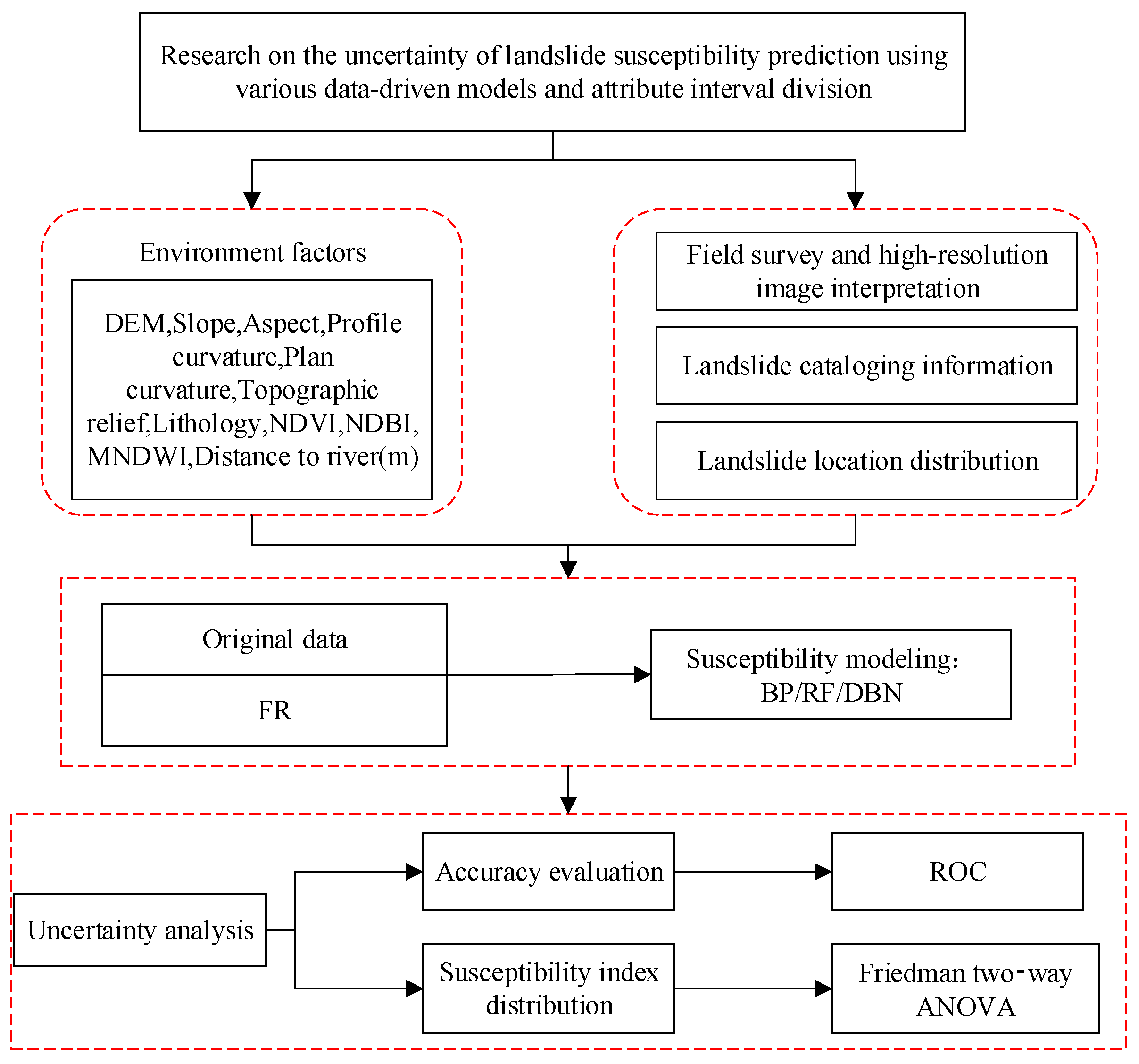
2.1. Research Ideas
- (1)
- The research area’s landslide catalog and associated environmental components were gathered (Figure 1). A FR analysis was then conducted using different AIN values for continuous environmental parameters (4, 8, 12, 16, 20);
- (2)
- The model training and test datasets are partitioned according to the most widely used 7:3 ratio, with the FR values of all the collected environmental parameters used as model input variables and the landslide catalog and randomly selected non-landslides used as output variables;
- (3)
- From the data-driven model, three models were chosen to forecast landslide susceptibility: DBN, RF, and BP;
- (4)
- In order to create 15 different situations, the FR values generated by 4 AIN were coupled with 3 different types of models. Susceptibility modeling was then completed;
- (5)
- The research area’s grid units’ landslide susceptibility indices were predicted and mapped using the established model;
- (6)
- Three perspectives were used to analyze the uncertainty of the prediction results: the receiver operation characteristic (ROC) curve accuracy evaluation, the susceptibility index difference, and its distribution law;
- (7)
- The value law of AIN in FR analysis was studied, and the effects of different kinds of data-driven models on predictability were examined.
2.2. Overview of Data-Driven Models
2.2.1. FR
2.2.2. RF
2.2.3. DBN
2.2.4. BP
2.3. Uncertainty Analysis Method
3. Application and Results
3.1. Geographical Environment Characteristics of Ruijin City
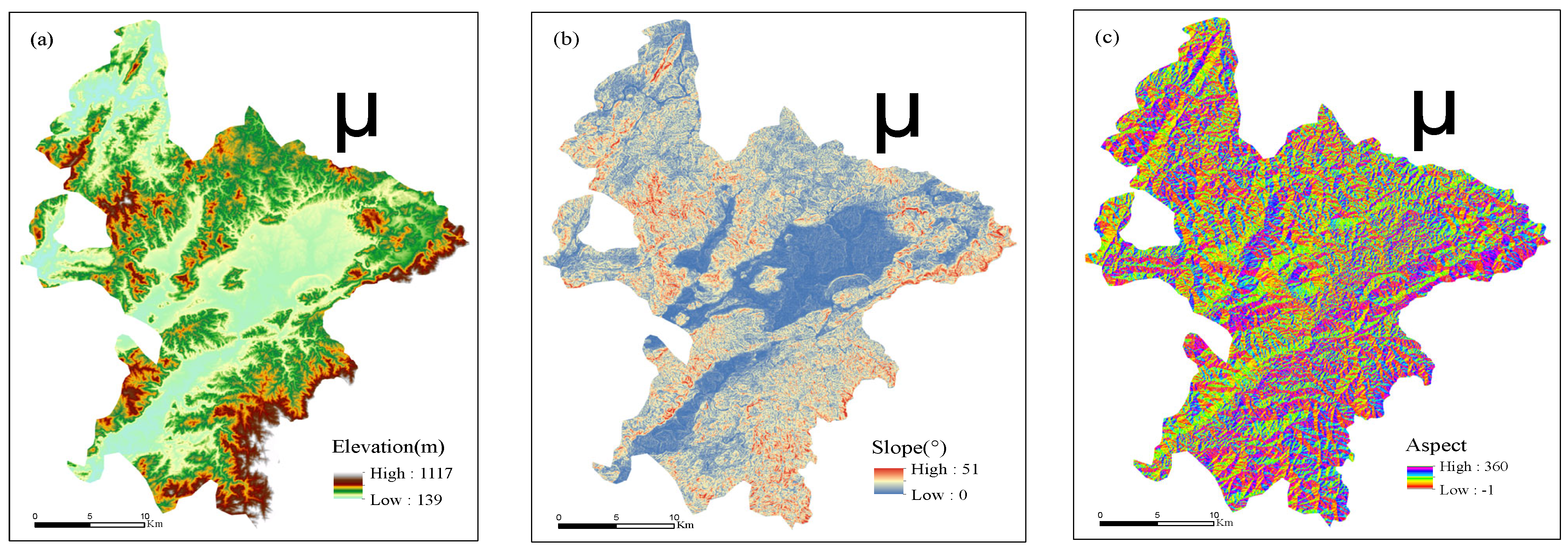
3.2. Landslide Catalogue and Its Environmental Factors
3.3. Landslide Susceptibility Prediction Unit
3.4. Environmental Factor Frequency Ratio Analysis
4. Landslide Susceptibility Prediction
4.1. Spatial Dataset Preparation
4.2. Susceptibility Prediction under Different AIN and Data-Driven Model Working Conditions
4.2.1. DBN Model Predicts Landslide Susceptibility
4.2.2. RF Models Forecast the Susceptibility to Landslides
4.2.3. BP Model Predicts Landslide Susceptibility
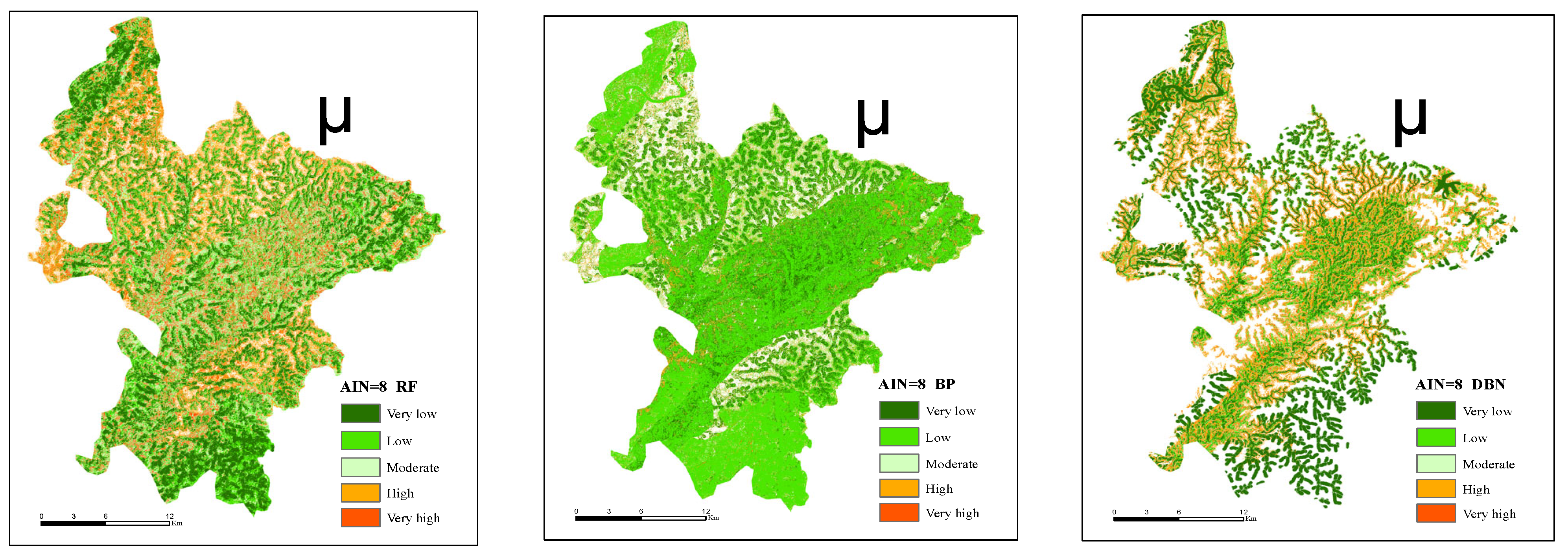
4.3. Landslide Susceptibility Mapping
5. Uncertainty Analysis of Susceptibility Prediction
5.1. Evaluation of Proximate Prediction Accuracy
5.2. Analysis of the Significance of Differences in Susceptibility Results
5.3. Distribution of Susceptibility Index under Typical Working Conditions
5.3.1. AIN Is 8 and Susceptibility Index Features under Different Models
5.3.2. Distribution Characteristics of Susceptibility Index of DBN Model and AIN Working Conditions
6. Discussion
7. Conclusions
- (1)
- When the frequency ratio analysis of the continuous environmental factor for landslides was conducted, the set AIN value increased from 4 to 8, and the accuracy of the susceptibility prediction increased quickly; when the AIN value increases from 8 to 20, the growth rate of susceptibility prediction accuracy slows down until it stabilizes. An important threshold for accurate prediction is an AIN value of 8, which can be used to avoid overly complex frequency ratio calculations.
- (2)
- The DBN model, followed by the RF and BP models, has the highest accuracy in predicting landslide susceptibility under all AIN working conditions, demonstrating that deep learning models can significantly increase the susceptibility prediction accuracy, and that the depth model typically outperforms shallow machine learning models in this regard.
- (3)
- When AIN value and data-driven models are combined, an AIN value of 20 and the DBN model have the highest prediction accuracy of landslide susceptibility, an AIN value of 4 and the BP model have the lowest accuracy, and an AIN value of 8 and the DBN model have the highest efficiency of landslide susceptibility prediction modeling.
- (4)
- This research also examines the uncertainty of vulnerability prediction modeling from the perspectives of the distinction significance of the landslide susceptibility index predicted by various working conditions and the distribution law of the susceptibility index, in addition to the AUC accuracy evaluation. The findings demonstrate that the projected landslide susceptibility index has reduced uncertainty and is more in accordance with the actual landslide probability distribution characteristics with larger AIN values and more sophisticated deep learning models such as DBN.
Author Contributions
Funding
Data Availability Statement
Acknowledgments
Conflicts of Interest
References
- Huang, F.; Zhang, J.; Zhou, C.; Wang, Y.; Huang, J.; Zhu, L. A deep learning algorithm using a fully connected sparse autoencoder neural network for landslide susceptibility prediction. Landslides 2020, 17, 217–229. [Google Scholar] [CrossRef]
- Dou, J.; Yunus, A.P.; Bui, D.T.; Merghadi, A.; Sahana, M.; Zhu, Z.; Chen, C.; Han, Z.; Pham, B.T. Improved landslide assessment using support vector machine with bagging, boosting, and stacking ensemble machine learning framework in a mountainous watershed, Japan. Landslides 2020, 17, 641–658. [Google Scholar] [CrossRef]
- Huang, F.; Cao, Z.; Jiang, S.H.; Zhou, C.; Huang, J.; Guo, Z. Landslide susceptibility prediction based on a semi-supervised multiple-layer perceptron model. Landslides 2020, 17, 2919–2930. [Google Scholar] [CrossRef]
- Khalaj, S.; BahooToroody, F.; Abaei, M.M.; BahooToroody, A.; De Carlo, F.; Abbassi, R. A methodology for uncertainty analysis of landslides triggered by an earthquake. Comput. Geotech. 2020, 117, 103262. [Google Scholar] [CrossRef]
- Ji, J.; Cui, H.; Zhang, T.; Song, J.; Gao, Y. A GIS-based tool for probabilistic physical modelling and prediction of landslides: GIS-FORM landslide susceptibility analysis in seismic areas. Landslides 2022, 19, 2213–2231. [Google Scholar] [CrossRef]
- Skrzypczak, I.; Kokoszka, W.; Zientek, D.; Tang, Y.; Kogut, J. Landslide hazard assessment map as an element supporting spatial planning: The flysch Carpathians region study. Remote Sens. 2021, 13, 317. [Google Scholar] [CrossRef]
- Shahri, A.A.; Spross, J.; Johansson, F.; Larsson, S. Landslide susceptibility hazard map in southwest Sweden using artificial neural network. Catena 2019, 183, 104225. [Google Scholar] [CrossRef]
- Saleem, N.; Huq, M.E.; Twumasi, N.Y.D.; Javed, A.; Sajjad, A. Parameters derived from and/or used with digital elevation models (DEMs) for landslide susceptibility mapping and landslide risk assessment: A review. ISPRS Int. J. Geo-Inf. 2019, 8, 545. [Google Scholar] [CrossRef]
- Myronidis, D.; Papageorgiou, C.; Theophanous, S. Landslide susceptibility mapping based on landslide history and analytic hierarchy process (AHP). Nat. Hazard. 2016, 81, 245–263. [Google Scholar] [CrossRef]
- Rahmati, O.; Kornejady, A.; Samadi, M.; Deo, R.C.; Conoscenti, C.; Lombardo, L.; Dayal, K.; Mehrjardi, R.T.; Bui, D.T. PMT: New analytical framework for automated evaluation of geo-environmental modelling approaches. Sci. Total Environ. 2019, 664, 296–311. [Google Scholar] [CrossRef]
- Alqadhi, S.; Mallick, J.; Talukdar, S.; Bindajam, A.A.; Van Hong, N.; Saha, T.K. Selecting optimal conditioning parameters for landslide susceptibility: An experimental research on Aqabat Al-Sulbat, Saudi Arabia. Environ. Sci. Pollut. Res. 2022, 29, 3743–3762. [Google Scholar] [CrossRef] [PubMed]
- Kornejady, A.; Ownegh, M.; Bahremand, A. Landslide susceptibility assessment using maximum entropy model with two different data sampling methods. Catena 2017, 152, 144–162. [Google Scholar] [CrossRef]
- Chowdhuri, I.; Pal, S.C.; Chakrabortty, R.; Malik, S.; Das, B.; Roy, P. Torrential rainfall-induced landslide susceptibility assessment using machine learning and statistical methods of eastern Himalaya. Nat. Hazard. 2021, 107, 697–722. [Google Scholar] [CrossRef]
- Dai, X.; Zhu, Y.; Sun, K.; Zou, Q.; Zhao, S.; Li, W.; Hu, L.; Wang, S. Examining the Spatially Varying Relationships between Landslide Susceptibility and Conditioning Factors Using a Geographical Random Forest Approach: A Case Study in Liangshan, China. Remote Sens. 2023, 15, 1513. [Google Scholar] [CrossRef]
- Xing, Y.; Yue, J.; Chen, C.; Cai, D.; Hu, J.; Xiang, Y. Prediction interval estimation of landslide displacement using adaptive chicken swarm optimization-tuned support vector machines. Appl. Intell. 2021, 51, 8466–8483. [Google Scholar] [CrossRef]
- Huang, F.; Cao, Z.; Guo, J.; Jiang, S.H.; Li, S.; Guo, Z. Comparisons of heuristic, general statistical and machine learning models for landslide susceptibility prediction and mapping. Catena 2020, 191, 104580. [Google Scholar] [CrossRef]
- Xing, Y.; Yue, J.; Chen, C.; Qin, Y.; Hu, J. A hybrid prediction model of landslide displacement with risk-averse adaptation. Comput. Geosci. 2020, 141, 104527. [Google Scholar] [CrossRef]
- Huang, F.; Chen, J.; Liu, W.; Huang, J.; Hong, H.; Chen, W. Regional rainfall-induced landslide hazard warning based on landslide susceptibility mapping and a critical rainfall threshold. Geomorphology 2022, 408, 108236. [Google Scholar] [CrossRef]
- Ada, M.; San, B.T. Comparison of machine-learning techniques for landslide susceptibility mapping using two-level random sampling (2LRS) in Alakir catchment area, Antalya, Turkey. Nat. Hazards 2018, 90, 237–263. [Google Scholar] [CrossRef]
- Jiang, S.H.; Huang, J.; Huang, F.; Yang, J.; Yao, C.; Zhou, C.B. Modelling of spatial variability of soil undrained shear strength by conditional random fields for slope reliability analysis. Appl. Math. Modell. 2018, 63, 374–389. [Google Scholar] [CrossRef]
- Chang, Z.; Catani, F.; Huang, F.; Yang, J.; Yao, C.; Zhou, C.B. Landslide susceptibility prediction using slope unit-based machine learning models considering the heterogeneity of conditioning factors. J. Rock Mech. Geotech. Eng. 2022, in press. [Google Scholar] [CrossRef]
- Xing, Y.; Yue, J.; Guo, Z.; Chen, Y.; Hu, J.; Travé, A. Large-scale landslide susceptibility mapping using an integrated machine learning model: A case study in the Lvliang mountains of China. Front. Earth Sci. 2021, 9, 622. [Google Scholar] [CrossRef]
- Xing, Y.; Yue, J.; Chen, C. Interval estimation of landslide displacement prediction based on time series decomposition and long short-term memory network. IEEE Access. 2019, 8, 3187–3196. [Google Scholar] [CrossRef]
- Chen, X.; Chen, W. GIS-based landslide susceptibility assessment using optimized hybrid machine learning methods. Catena 2021, 196, 104833. [Google Scholar] [CrossRef]
- Zhu, A.X.; Miao, Y.; Liu, J.; Bai, S.; Zeng, C.; Ma, T.; Hong, H. A similarity-based approach to sampling absence data for landslide susceptibility mapping using data-driven methods. Catena 2019, 183, 104188. [Google Scholar] [CrossRef]
- Dou, J.; Yunus, A.P.; Xu, Y.; Zhu, Z.; Chen, C.W.; Sahana, M.; Khosravi, K.; Yang, Y.; Pham, B.T. Torrential rainfall-triggered shallow landslide characteristics and susceptibility assessment using ensemble data-driven models in the Dongjiang Reservoir Watershed, China. Nat. Hazard. 2019, 97, 579–609. [Google Scholar] [CrossRef]
- Lin, Q.; Lima, P.; Steger, S.; Glade, T.; Jiang, T.; Zhang, J.; Liu, T.; Wang, Y. National-scale data-driven rainfall induced landslide susceptibility mapping for China by accounting for incomplete landslide data. Geosci. Front. 2021, 12, 101248. [Google Scholar] [CrossRef]
- Hong, H.; Liu, J.; Zhu, A.X. Modeling landslide susceptibility using LogitBoost alternating decision trees and forest by penalizing attributes with the bagging ensemble. Sci. Total Environ. 2020, 718, 137231. [Google Scholar] [CrossRef]
- Tehrani, F.S.; Calvello, M.; Liu, Z.; Zhang, L.; Lacasse, S. Machine learning and landslide studies: Recent advances and applications. Nat. Hazard. 2022, 114, 1197–1245. [Google Scholar] [CrossRef]
- Chen, W.; Pourghasemi, H.R.; Panahi, M.; Kornejady, A.; Wang, J.; Xie, X.; Cao, S. Spatial prediction of landslide susceptibility using an adaptive neuro-fuzzy inference system combined with frequency ratio, generalized additive model, and support vector machine techniques. Geomorphology 2017, 297, 69–85. [Google Scholar] [CrossRef]
- Wankhade, M.; Rao, A.C.S.; Kulkarni, C. A survey on sentiment analysis methods, applications, and challenges. Artif. Intell. Rev. 2022, 55, 5731–5780. [Google Scholar]
- Mrówczyńska, M.; Skiba, M.; Leśniak, A.; Bazan-Krzywoszańska, A.; Janowiec, F.; Sztubecka, M.; Grech, R.; Kazak, J.K. A new fuzzy model of multi-criteria decision support based on Bayesian networks for the urban areas’ decarbonization planning. Energy Convers. Manag. 2022, 268, 116035. [Google Scholar] [CrossRef]
- Aidinidou, M.T.; Kaparis, K.; Georgiou, A.C. Analysis, prioritization and strategic planning of flood mitigation projects based on sustainability dimensions and a spatial/value AHP-GIS system. Expert Syst. Appl. 2023, 211, 118566. [Google Scholar] [CrossRef]
- El-Haddad, B.A.; Youssef, A.M.; Pourghasemi, H.R.; Pradhan, B.; El-Shater, A.H.; El-Khashab, M.H. Flood susceptibility prediction using four machine learning techniques and comparison of their performance at Wadi Qena Basin, Egypt. Nat. Hazard. 2021, 105, 83–114. [Google Scholar] [CrossRef]
- Kmoch, A.; Kanal, A.; Astover, A.; Kull, A.; Virro, H.; Helm, A.; Pärtel, M.; Ostonen, L.; Uuemaa, E. EstSoil-EH: A high-resolution eco-hydrological modelling parameters dataset for Estonia. Earth Syst. Sci. Data 2021, 13, 83–97. [Google Scholar] [CrossRef]
- Tahan, M.; Tsoutsanis, E.; Muhammad, M.; Karim, Z.A.A. Performance-based health monitoring, diagnostics and prognostics for condition-based maintenance of gas turbines: A review. Appl. Energy 2017, 198, 122–144. [Google Scholar] [CrossRef]
- Huang, F.; Yan, J.; Fan, X.; Yao, C.; Huang, J.; Chen, W.; Hong, H. Uncertainty pattern in landslide susceptibility prediction modelling: Effects of different landslide boundaries and spatial shape expressions. Geosci. Front. 2022, 13, 101317. [Google Scholar] [CrossRef]
- Reichstein, M.; Camps-Valls, G.; Stevens, B.; Jung, M.; Denzler, J.; Carvalhais, N.; Parbha, P. Deep learning and process understanding for data-driven Earth system science. Nature 2019, 566, 195–204. [Google Scholar] [CrossRef]
- Xia, M.; Zheng, X.; Imran, M.; Shoaib, M. Data-driven prognosis method using hybrid deep recurrent neural network. Appl. Soft Comput. 2020, 93, 106351. [Google Scholar] [CrossRef]
- Rajabi, A.M.; Khodaparast, M.; Mohammadi, M. Earthquake-induced landslide prediction using back-propagation type artificial neural network: Case study in northern Iran. Nat. Hazard. 2022, 110, 679–694. [Google Scholar] [CrossRef]
- Pradhan, B. A comparative study on the predictive ability of the decision tree, support vector machine and neuro-fuzzy models in landslide susceptibility mapping using GIS. Comput. Geosci. 2013, 51, 350–365. [Google Scholar] [CrossRef]
- Goetz, J.N.; Brenning, A.; Petschko, H.; Leopold, P. Evaluating machine learning and statistical prediction techniques for landslide susceptibility modeling. Comput. Geosci. 2015, 81, 1–11. [Google Scholar] [CrossRef]
- Huang, Y.; Zhao, L. Review on landslide susceptibility mapping using support vector machines. Catena 2018, 165, 520–529. [Google Scholar] [CrossRef]
- Lee, J.H.; Kim, H.; Park, H.J.; Heo, J.H. Temporal prediction modeling for rainfall-induced shallow landslide hazards using extreme value distribution. Landslides 2021, 18, 321–338. [Google Scholar] [CrossRef]
- Guo, Z.; Shi, Y.; Huang, F.; Fan, X.; Huang, J. Landslide susceptibility zonation method based on C5. 0 decision tree and K-means cluster algorithms to improve the efficiency of risk management. Geosci. Front. 2021, 12, 101249. [Google Scholar] [CrossRef]
- Samia, J.; Temme, A.; Bregt, A.; Wallinga, J.; Guzzetti, F.; Ardizzone, F.; Rossi, M. Do landslides follow landslides? Insights in path dependency from a multi-temporal landslide inventory. Landslides 2017, 14, 547–558. [Google Scholar] [CrossRef]
- Arabameri, A.; Pradhan, B.; Rezaei, K.; Lee, C.W. Assessment of landslide susceptibility using statistical-and artificial intelligence-based FR—RF integrated model and multiresolution DEMs. Remote Sens. 2019, 11, 999. [Google Scholar] [CrossRef]
- Hu, X.; Wu, S.; Zhang, G.; Zheng, W.; Liu, C.; He, C.; Liu, Z.; Guo, X.; Zhang, H. Landslide displacement prediction using kinematics-based random forests method: A case study in Jinping Reservoir Area, China. Eng. Geol. 2021, 283, 105975. [Google Scholar] [CrossRef]
- Zhao, Z.; Liu, Z.Y.; Xu, C. Slope unit-based landslide susceptibility mapping using certainty factor, support vector machine, random forest, CF-SVM and CF-RF models. Front. Earth Sci. 2021, 9, 589630. [Google Scholar] [CrossRef]
- Fang, Z.; Wang, Y.; Niu, R.; Peng, L. Landslide susceptibility prediction based on positive unlabeled learning coupled with adaptive sampling. IEEE J. Sel. Top. Appl. Earth Obs. Remote Sens. 2021, 14, 11581–11592. [Google Scholar] [CrossRef]
- Pourghasemi, H.R.; Rahmati, O. Prediction of the landslide susceptibility: Which algorithm, which precision? Catena 2018, 162, 177–192. [Google Scholar] [CrossRef]
- Li, H.; Xu, Q.; He, Y.; Fan, X.; Li, S. Modeling and predicting reservoir landslide displacement with deep belief network and EWMA control charts: A case study in Three Gorges Reservoir. Landslides 2020, 17, 693–707. [Google Scholar] [CrossRef]
- Guo, Z.; Chen, L.; Gui, L.; Du, J.; Yin, K.; Do, H.M. Landslide displacement prediction based on variational mode decomposition and WA-GWO-BP model. Landslides 2020, 17, 567–583. [Google Scholar] [CrossRef]
- Xu, S.; Niu, R. Displacement prediction of Baijiabao landslide based on empirical mode decomposition and long short-term memory neural network in Three Gorges area, China. Comput. Geosci. 2018, 111, 87–96. [Google Scholar] [CrossRef]
- Medina, V.; Hürlimann, M.; Guo, Z.; Lloret, A.; Vaunat, J. Fast physically-based model for rainfall-induced landslide susceptibility assessment at regional scale. Catena 2021, 201, 105213. [Google Scholar] [CrossRef]
- Van Dao, D.; Jaafari, A.; Bayat, M.; Mafi-Gholami, D.; Qi, C.; Moayedi, H.; Van Phong, T.; Ly, H.B.; Le, T.T.; Trong Trinh, P. A spatially explicit deep learning neural network model for the prediction of landslide susceptibility. Catena 2020, 188, 104451. [Google Scholar]
- Chang, Z.; Du, Z.; Zhang, F.; Huang, F.; Chen, J.; Li, W.; Guo, Z. Landslide susceptibility prediction based on remote sensing images and GIS: Comparisons of supervised and unsupervised machine learning models. Remote Sens. 2020, 12, 502. [Google Scholar] [CrossRef]
- Zhao, X.; Chen, W. Optimization of computational intelligence models for landslide susceptibility evaluation. Remote Sens. 2020, 12, 2180. [Google Scholar] [CrossRef]
- Conoscenti, C.; Ciaccio, M.; Caraballo-Arias, N.A.; Gómez-Gutiérrez, Á.; Rotigliano, E.; Agnesi, V. Assessment of susceptibility to earth-flow landslide using logistic regression and multivariate adaptive regression splines: A case of the Belice River basin (western Sicily, Italy). Geomorphology 2015, 242, 49–64. [Google Scholar] [CrossRef]
- Zou, Q.; Jiang, H.; Cui, P.; Zhou, B.; Jiang, Y.; Qin, M.; Liu, Y.; Li, C. A new approach to assess landslide susceptibility based on slope failure mechanisms. Catena 2021, 204, 105388. [Google Scholar] [CrossRef]
- Geertsema, M.; Highland, L.; Vaugeouis, L. Environmental impact of landslides. In Landslides—Disaster Risk Reduction; Springer: Cham, Switzerland, 2009; pp. 589–607. [Google Scholar]
- Lucchese, L.V.; de Oliveira, G.G.; Pedrollo, O.C. Mamdani fuzzy inference systems and artificial neural networks for landslide susceptibility mapping. Nat. Hazard. 2021, 106, 2381–2405. [Google Scholar] [CrossRef]
- Lima, P.; Steger, S.; Glade, T. Counteracting flawed landslide data in statistically based landslide susceptibility modelling for very large areas: A national-scale assessment for Austria. Landslides 2021, 18, 3531–3546. [Google Scholar] [CrossRef]
- Ly, H.B.; Nguyen, M.H.; Pham, B.T. Metaheuristic optimization of Levenberg—Marquardt-based artificial neural network using particle swarm optimization for prediction of foamed concrete compressive strength. Neural Comput. Appl. 2021, 33, 17331–17351. [Google Scholar] [CrossRef]


| No. Data | Scale/Resolution | Source | Purpose |
|---|---|---|---|
| DEM | 25 m | China Geological Survey (Jiangxi Center) | Causal factor maps |
| Topographic map | 1:50,000 | ||
| Geological map | 1:100,000 | ||
| Urban planning map | 1:100,000 | Department of Survey and Mapping of Jiangxi Province | Land use, normalized difference vegetation index, and soil erosion intensity maps |
| Environmental planning map | 1:100,000 | ||
| Remote sensing images | 15 m | Landslide TM | |
| Rainfall | Monthly data | Department of Meteorology of Jiangxi Province | Rainfall distribution map |
| Landslide reports | / | China Geological Survey (Jiangxi Center) | Landslide inventory map |
| Landslide photos | 2048 × 1536 dpi | Drone | |
| Remote sensing images | 30 m | Google Earth |
| Influence Factor | AIN = 4 | AIN = 8 | AIN = 12 | AIN = 16 | AIN = 20 | |||||
|---|---|---|---|---|---|---|---|---|---|---|
| Attribute Interval | FR | Attribute Interval | FR | Attribute Interval | FR | Attribute Interval | FR | Attribute Interval | FR | |
| DEM | 139–278 | 1.494 | 139–239 | 1.547 | 139–228 | 1.675 | 139–213 | 1.984 | 139–205 | 2.116 |
| 278–401 | 0.839 | 239–308 | 1.229 | 228–282 | 1.268 | 213–259 | 1.140 | 205–243 | 1.234 | |
| 401–581 | 0.488 | 308–374 | 0.839 | 282–335 | 1.022 | 259–305 | 1.197 | 243–285 | 1.295 | |
| 581–1117 | 0.249 | 374–447 | 0.503 | 335–385 | 0.631 | 305–351 | 0.910 | 285–324 | 1.036 | |
| 447–535 | 0.481 | 385–439 | 0.559 | 351–397 | 0.593 | 324–366 | 0.816 | |||
| 535–642 | 0.306 | 439–496 | 0.530 | 397–447 | 0.555 | 366–408 | 0.721 | |||
| 642–780 | 0.225 | 496–558 | 0.326 | 447–496 | 0.584 | 408–450 | 0.371 | |||
| 780–1117 | 0.289 | 558–623 | 0.316 | 496–546 | 0.305 | 450–493 | 0.575 | |||
| 623–696 | 0 | 556–599 | 0.225 | 493–539 | 0.314 | |||||
| 696–776 | 0.465 | 599–654 | 0.329 | 539–585 | 0.239 | |||||
| 776–880 | 0 | 654–707 | 0 | 585–631 | 0.510 | |||||
| 880–1117 | 0.934 | 707–761 | 0.341 | 631–677 | 0 | |||||
| 761–842 | 0.526 | 677–723 | 0 | |||||||
| 842–876 | 0 | 723–769 | 0.858 | |||||||
| 876–953 | 1.379 | 769–815 | 0 | |||||||
| 953–1117 | 0 | 815–861 | 0 | |||||||
| 861–907 | 0 | |||||||||
| 907–957 | 2.638 | |||||||||
| 957–1010 | 0 | |||||||||
| 1010–1117 | 0 | |||||||||
| Slope | 0–6 | 0.613 | 0–4 | 0.326 | 0–3 | 0.248 | 0–3 | 0.234 | 0–2 | 0.217 |
| 6–12 | 1.503 | 4–7 | 1.229 | 3–6 | 1.190 | 3–5 | 0.934 | 2–4 | 0.673 | |
| 12–19 | 1.013 | 7–11 | 1.632 | 6–9 | 1.629 | 5–8 | 1.424 | 4–7 | 1.271 | |
| 19–51 | 0.566 | 11–14 | 1.255 | 9–12 | 1.306 | 8–11 | 1.704 | 7–9 | 1.698 | |
| 14–18 | 0.813 | 12–15 | 1.164 | 11–13 | 1.184 | 9–11 | 1.356 | |||
| 18–22 | 0.807 | 15–17 | 0.817 | 13–15 | 1.089 | 11–14 | 1.281 | |||
| 22–27 | 0.551 | 17–20 | 0.812 | 15–17 | 0.786 | 14–16 | 0.863 | |||
| 27–51 | 0.575 | 20–23 | 0.698 | 17–19 | 1.089 | 16–18 | 0.981 | |||
| 23–25 | 0.672 | 19–21 | 0.524 | 18–20 | 0.897 | |||||
| 25–29 | 0.602 | 21–23 | 0.647 | 20–22 | 0.725 | |||||
| 29–33 | 0.429 | 23–25 | 0.614 | 22–23 | 0.636 | |||||
| 33–51 | 0 | 25–28 | 0.723 | 23–25 | 0.564 | |||||
| 28–30 | 0 | 25–27 | 0.287 | |||||||
| 30–33 | 0.841 | 27–29 | 0.934 | |||||||
| 33–37 | 0 | 29–31 | 0.795 | |||||||
| 37–51 | 0 | 31–33 | 0 | |||||||
| 33–35 | 0 | |||||||||
| 35–37 | 0 | |||||||||
| 37–40 | 0 | |||||||||
| 40–51 | 0 | |||||||||
| Influence Factor | AIN = 4 | AIN = 8 | AIN = 12 | AIN = 16 | AIN = 20 | |||||
|---|---|---|---|---|---|---|---|---|---|---|
| Attribute Interval | FR | Attribute Interval | FR | Attribute Interval | FR | Attribute Interval | FR | Attribute Interval | FR | |
| MNDWI | −0.035–0.137 | 1.115 | −0.035–0.097 | 1.120 | −0.035–0.070 | 0.495 | −0.035–0.049 | 0 | −0.035–0.039 | 0 |
| 0.137–0.209 | 0.953 | 0.097–0.142 | 1.109 | 0.070–0.110 | 1.133 | 0.049–0.084 | 1.068 | 0.039–0.068 | 0.628 | |
| 0.209–0.297 | 1.009 | 0.142–0.182 | 0.907 | 0.110–0.142 | 1.229 | 0.084–0.110 | 1.094 | 0.068–0.092 | 1.457 | |
| 0.297–0.643 | 0.866 | 0.182–0.225 | 0.998 | 0.142–0.172 | 0.896 | 0.110–0.137 | 1.262 | 0.092–0.116 | 0.849 | |
| 0.225–0.270 | 0.979 | 0.172–0.201 | 0.897 | 0.137–0.164 | 1.029 | 0.116–0.139 | 1.338 | |||
| 0.270–0.321 | 0.892 | 0.201–0.233 | 1.130 | 0.164–0.190 | 0.786 | 0.139–0.161 | 0.999 | |||
| 0.321–0.387 | 0.840 | 0.233–0.265 | 0.956 | 0.190–0.217 | 1.044 | 0.161–0.185 | 0.862 | |||
| 0.387–0.643 | 1.587 | 0.265–0.299 | 1.006 | 0.217–0.246 | 0.969 | 0.185–0.209 | 0.991 | |||
| 0.299–0.337 | 0.791 | 0.246–0.276 | 1.075 | 0.209–0.236 | 1.033 | |||||
| 0.337–0.379 | 0.665 | 0.276–0.305 | 0.947 | 0.236–0.259 | 0.989 | |||||
| 0.379–0.432 | 0.830 | 0.305–0.334 | 0.861 | 0.259–0.284 | 1.047 | |||||
| 0.432–0.643 | 2.734 | 0.334–0.364 | 0.554 | 0.284–0.310 | 0.674 | |||||
| 0.364–0.395 | 0.878 | 0.310–0.337 | 1.010 | |||||||
| 0.395–0.430 | 1.097 | 0.337–0.364 | 0.467 | |||||||
| 0.430–0.473 | 2.667 | 0.364–0.390 | 0.757 | |||||||
| 0.473–0.643 | 1.857 | 0.390–0.417 | 0.801 | |||||||
| 0.417–0.443 | 4.087 | |||||||||
| 0.443–0.473 | 0 | |||||||||
| 0.473–0.507 | 2.490 | |||||||||
| 0.507–0.643 | 0 | |||||||||
| Influence Factor | AIN = 4 | AIN = 8 | AIN = 12 | AIN = 16 | AIN = 20 | |||||
|---|---|---|---|---|---|---|---|---|---|---|
| Attribute Interval | FR | Attribute Interval | FR | Attribute Interval | FR | Attribute Interval | FR | Attribute Interval | FR | |
| NDVI | −0.054–0.016 | 0.759 | −0.054–0.000 | 0.868 | −0.054–−0.007 | 0 | −0.054–−0.019 | 0 | −0.054–−0.028 | 0 |
| 0.016–0.027 | 0.883 | 0.000–0.011 | 0.681 | −0.007–0.002 | 1.194 | −0.019–−0.009 | 0 | −0.028–−0.019 | 0 | |
| 0.027–0.038 | 1.180 | 0.011–0.018 | 0.901 | 0.002–0.009 | 0.739 | −0.009–−0.003 | 1.576 | −0.019–−0.012 | 0 | |
| 0.038–0.097 | 0.958 | 0.018–0.025 | 0.684 | 0.009–0.014 | 0.888 | −0.003–0.003 | 0.367 | −0.012–−0.006 | 3.181 | |
| 0.025–0.031 | 1.218 | 0.014–0.019 | 0.795 | 0.003–0.007 | 0.548 | −0.006–−0.002 | 0 | |||
| 0.031–0.038 | 1.153 | 0.019–0.024 | 0.689 | 0.007–0.012 | 1.176 | −0.002–0.002 | 0.433 | |||
| 0.038–0.046 | 1.191 | 0.024–0.029 | 1.128 | 0.012–0.017 | 0.600 | 0.002–0.007 | 0.441 | |||
| 0.046–0.097 | 0.444 | 0.029–0.033 | 1.207 | 0.017–0.021 | 0.748 | 0.007–0.011 | 0.891 | |||
| 0.033–0.038 | 1.113 | 0.021–0.026 | 0.740 | 0.011–0.015 | 0.831 | |||||
| 0.038–0.043 | 0.972 | 0.026–0.029 | 1.332 | 0.015–0.019 | 0.896 | |||||
| 0.043–0.049 | 1.133 | 0.029–0.034 | 1.187 | 0.019–0.024 | 0.648 | |||||
| 0.049–0.097 | 0.546 | 0.034–0.039 | 1.069 | 0.024–0.028 | 1.145 | |||||
| 0.039–0.044 | 0.996 | 0.028–0.032 | 1.204 | |||||||
| 0.044–0.049 | 1.248 | 0.032–0.036 | 1.082 | |||||||
| 0.049–0.054 | 0.441 | 0.036–0.041 | 0.965 | |||||||
| 0.054–0.097 | 0.332 | 0.041–0.044 | 1.344 | |||||||
| 0.044–0.048 | 1.113 | |||||||||
| 0.048–0.052 | 0.457 | |||||||||
| 0.052–0.057 | 0.511 | |||||||||
| 0.057–0.097 | 0 | |||||||||
| Input | Hidden | Output | Samples | Training Method | Iterations | Learning Rate | Error | ||
|---|---|---|---|---|---|---|---|---|---|
| 11 | 15 | 1 | 3000 | Logsig | Purelin | LM | 1000 | 0.01 | 0.01 |
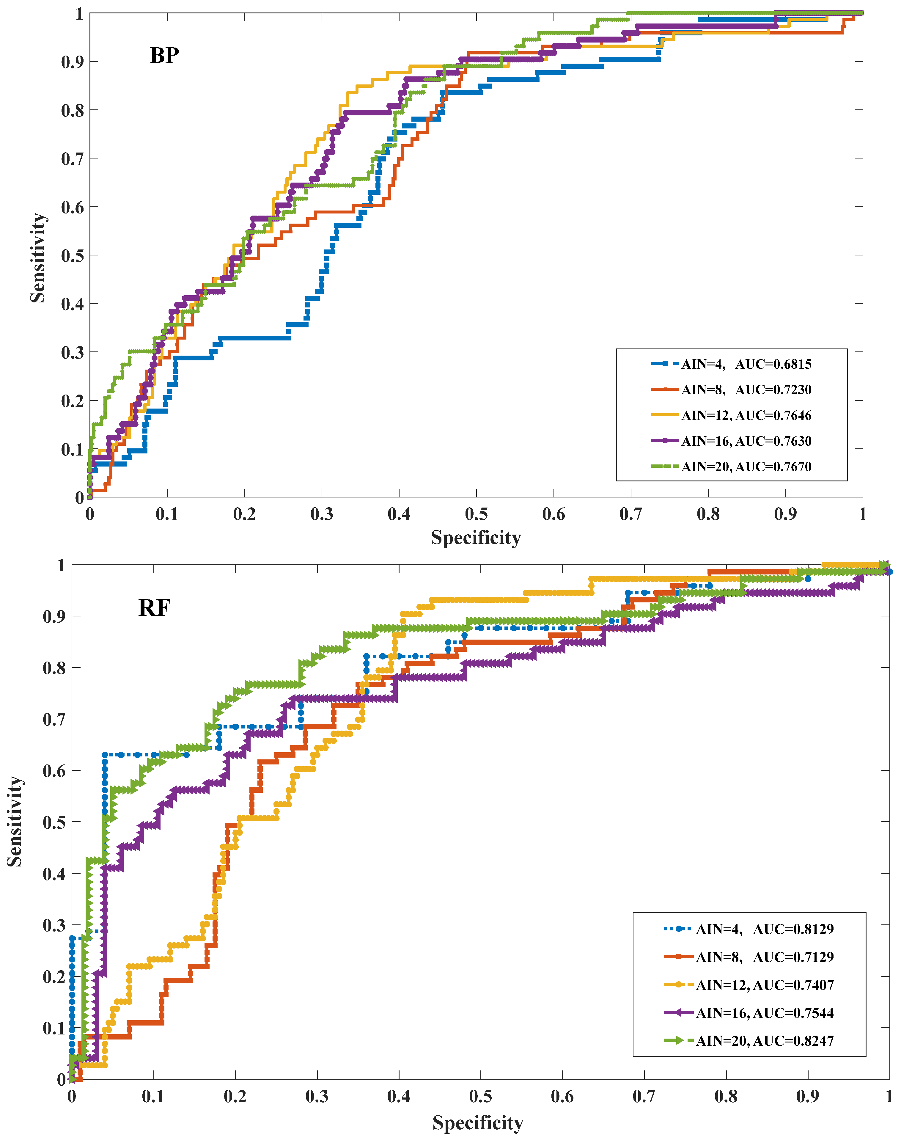
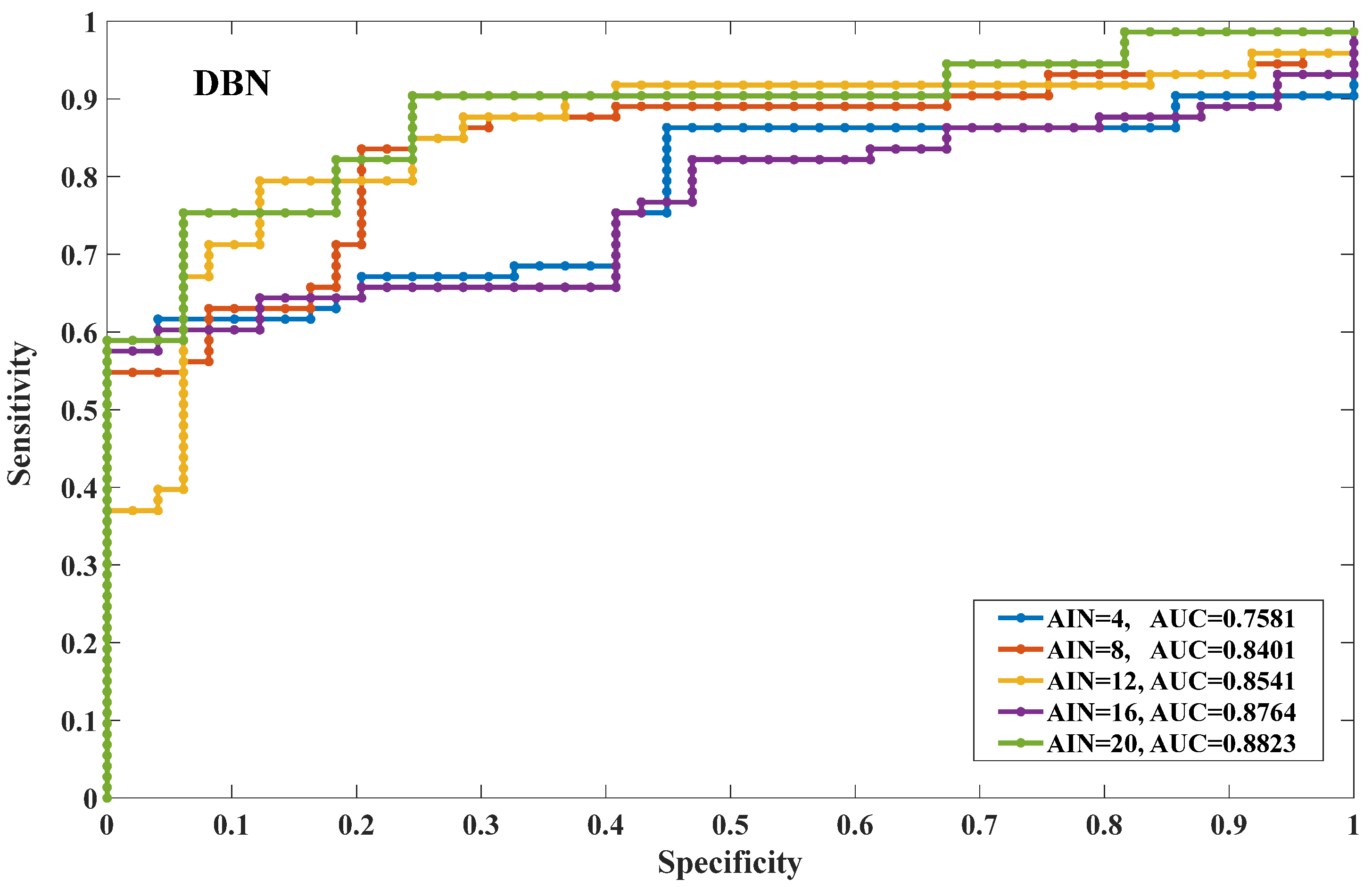
| Model | AIN | ||||
|---|---|---|---|---|---|
| 4 | 8 | 12 | 16 | 20 | |
| BP | 0.6815 | 0.7230 | 0.7646 | 0.7630 | 0.7670 |
| RF | 0.8129 | 0.7129 | 0.7407 | 0.7544 | 0.8247 |
| DBN | 0.7581 | 0.8401 | 0.8541 | 0.8764 | 0.8823 |
| Modeling Conditions | AIN Comparison | Significance | AIN Comparison | Significance | AIN Comparison | Significance | AIN Comparison | Significance |
|---|---|---|---|---|---|---|---|---|
| Different AIN and DBN models | 4, 8 | 1.000 | ||||||
| 4, 12 | 0.036 | 8, 12 | 0.556 | |||||
| 4, 16 | 0.036 | 8, 16 | 1.000 | 12, 16 | 1.000 | |||
| 4, 20 | 0.005 | 8, 20 | 0.165 | 16, 20 | 1.000 | 16, 20 | 1.000 | |
| Modeling Conditions | Model Comparison | Significance | Model Comparison | Significance | ||||
| AIN = 8 and different models | DBN, BP | 0.036 | ||||||
| DBN, RF | 0.045 | BP, RF | 1.000 |
Disclaimer/Publisher’s Note: The statements, opinions and data contained in all publications are solely those of the individual author(s) and contributor(s) and not of MDPI and/or the editor(s). MDPI and/or the editor(s) disclaim responsibility for any injury to people or property resulting from any ideas, methods, instructions or products referred to in the content. |
© 2023 by the authors. Licensee MDPI, Basel, Switzerland. This article is an open access article distributed under the terms and conditions of the Creative Commons Attribution (CC BY) license (https://creativecommons.org/licenses/by/4.0/).
Share and Cite
Xing, Y.; Chen, Y.; Huang, S.; Xie, W.; Wang, P.; Xiang, Y. Research on the Uncertainty of Landslide Susceptibility Prediction Using Various Data-Driven Models and Attribute Interval Division. Remote Sens. 2023, 15, 2149. https://doi.org/10.3390/rs15082149
Xing Y, Chen Y, Huang S, Xie W, Wang P, Xiang Y. Research on the Uncertainty of Landslide Susceptibility Prediction Using Various Data-Driven Models and Attribute Interval Division. Remote Sensing. 2023; 15(8):2149. https://doi.org/10.3390/rs15082149
Chicago/Turabian StyleXing, Yin, Yang Chen, Saipeng Huang, Wei Xie, Peng Wang, and Yunfei Xiang. 2023. "Research on the Uncertainty of Landslide Susceptibility Prediction Using Various Data-Driven Models and Attribute Interval Division" Remote Sensing 15, no. 8: 2149. https://doi.org/10.3390/rs15082149