Mapping and Influencing the Mechanism of CO₂ Emissions from Building Operations Integrated Multi-Source Remote Sensing Data

Abstract

Urbanization has led to rapid growth in energy consumption and CO₂ emissions in the building sector. Building operation emissions (BCEs) are a major part of emissions in the building life cycle. Existing studies have attempted to estimate fine-scale BCEs using remote sensing data. However, there is still a lack of research on estimating long-term BCEs by integrating multi-source remote sensing data and applications in different regions. We selected the Beijing–Tianjin–Hebei (BTH) urban agglomeration and the National Capital Region of Japan (NCRJ) as research areas for this study. We also built multiple linear regression (MLR) models between prefecture-level BCEs and multi-source remote sensing data. The prefecture-level BCEs were downscaled to grid scale at a 1 km² resolution. The estimation results verify the method’s difference and accuracy at different development stages. The multi-scale BCEs showed a continuous growth trend in the BTH urban agglomeration and a significant downward trend in the NCRJ. The decrease in energy intensity and population density were the main factors contributing to the negative growth of BCEs, whereas GDP per capita and urban expansion significantly promoted it. Through our methods and analyses, we contribute to the study of estimating greenhouse gas emissions with remote sensing and exploring the environmental impact of urban growth.

1. Introduction

Global urbanization has accelerated since the 1950s, with more than 50% of the current population living in urban areas, which is expected to reach 68% by 2050 [1]. Meanwhile, carbon dioxide (CO₂) emissions from energy consumption have increased significantly, with global energy-related CO₂ emissions exceeding 36 billion tons in 2021 [2]. Since buildings are the main carriers of population and economic activities, energy consumption and CO₂ related to building operations reached 35 and 38% globally, respectively; furthermore, CO₂ from building operations accounted for 30 and 28% globally [3]. Given the high share and growth trend of buildings’ energy demand and CO₂ emissions under rapid urbanization, reduced energy conservation and emissions in the building sector play an important role in promoting low-carbon cities [4].

1.1. Calculation of CO₂ Emissions from the Building Sector

Life cycle assessments have been widely used to determine buildings’ energy consumption and CO₂ emissions [5,6,7,8]. The life cycle assessment of buildings was divided into three main parts: the processing and construction, operation, and demolition stages [5,9]. Besides estimating CO₂ emissions [10,11,12,13,14], existing studies analyzed the emissions between residential and commercial buildings using various materials at different stages of the building life cycle [6,9]. Based on estimating office buildings’ emissions at the construction stage, building height positively promoted unit area emissions [15]. In addition to life cycle assessments, previous studies estimated buildings’ CO₂ emissions at different stages, such as material input, energy consumption, and human input, using input–output methods [16,17,18]. By comparing emissions at different stages, researchers found that energy consumption in the operation stage accounted for the highest proportion in the building’s whole life cycle [6,7,9,19].

The operation stage mainly includes the energy consumed by heating, air conditioning, lighting, and other functions of residential, commercial, and office buildings [20]. The operation stage is the main source of energy consumption and CO₂ emissions in the life cycle of a building. Previous studies focused on estimating energy consumption and CO₂ emissions at the operation stage using China’s building energy consumption calculation method (CBECM). This method extracted energy consumption related to building operations from sector statistics in the energy balance sheet [21]. For the fine-scale emissions of building operations in China, a regression model was established between building operation emissions, air temperature, and economic factors at the provincial level and downscaled them to a 1 km resolution [22]. A combined energy balance sheet with POI weights and CO₂ emissions from building operations in Beijing was mapped at a grid scale [23]. Nighttime light data have been widely used to estimate energy consumption and CO₂ emissions [24,25,26,27,28,29]. Previous studies have proven its effectiveness in evaluating buildings’ material stocks [30,31] and have also used the linear regression model to downscale the building sector’s carbon emissions in the United Kingdom [32]. In addition, nighttime light data could explain more than 90% of the variation in building energy consumption in the United States [26].

1.2. Influencing Factors of CO₂ Emissions from the Building Sector

Natural and socioeconomic factors affect energy consumption and CO₂ at the buildings’ operation stage [33,34]. Table 1 lists the building emissions’ influencing factors from natural and socioeconomic dimensions. Under the background of climate warming, the rise in temperature causes increased demand for cooling and lower demand for heating [35]. However, the decrease in emissions due to less heating could be negated by cooling if there is no limitation to using air conditioning [36]. Existing studies explored the urban heat island’s effect on buildings’ energy consumption and found that the energy consumption of urban buildings for cooling in summer was higher than that of suburban buildings. However, energy consumption for heating was reversed in winter [37]. With the rapid urbanization process, vegetation cover loss is significant. Previous studies have indicated a positive correlation between vegetation cover loss and land surface temperature, which exacerbates the urban heat island effect and affects building energy consumption indirectly [38,39]. The geographical location affects a region’s BCEs by determining energy endowments and climatic characteristics, causing different energy consumption constructures and energy demands between regions [40,41].

Energy demand and CO₂ emissions from buildings are affected by urbanization, with urban growth increasing the demand for central heating in winter and refrigeration in summer [42,43,44]. Previous studies compared the impacts of population, economic, and spatial urbanization on building energy consumption, with population urbanization having the strongest positive effect [40,45]. As for factors influencing CO₂ from China’s building sector, Logarithmic Mean Divisia index (LMDI) model results revealed the positive effect of the tertiary sector, indicating that an increase in consumption has driven significant CO₂ emission increases from buildings [41,46]. Similarly, residents’ lifestyles represent an important factor affecting building energy consumption because of different income levels and energy structures [47,48]. Improvements in the energy structure and technological progress could effectively reduce BCEs [49,50]. Land development, which is used for commercial and residential land, has a positive effect on building CO₂ emissions [42,50]. In addition, previous studies compared factors influencing residential and commercial buildings. Their results showed that newer, higher-quality commercial buildings require more electricity than residential buildings [51]. Residential energy intensity and the energy-saving policies of commercial buildings promote the decoupling effect of CO₂ emissions from residential and commercial buildings, respectively [52,53].

Table 1. Influencing factors in previous studies.

Dimension	Influencing Factors	Influencing Results
Natural factors	temperature [35,36,37]	positive (summer)/negative (winter)
	less vegetation cover [38,39]	positive
	geographical location [41]	/
Socioeconomic factors	urbanization [40,45]	positive
	economic growth [41]	positive
	tertiary industry [41,46]	positive
	population [40,54]	positive
	technological progress [49,50]	negative
	urban land use [42,50]	positive

Table 1. Influencing factors in previous studies.

Dimension	Influencing Factors	Influencing Results
Natural factors	temperature [35,36,37]	positive (summer)/negative (winter)
	less vegetation cover [38,39]	positive
	geographical location [41]	/
Socioeconomic factors	urbanization [40,45]	positive
	economic growth [41]	positive
	tertiary industry [41,46]	positive
	population [40,54]	positive
	technological progress [49,50]	negative
	urban land use [42,50]	positive

Emission reduction in the building sector is important for promoting the carbon peak and carbon neutrality. Although studies have attempted to determine fine-scale estimations of BCEs using remote sensing data, those exploring multi-source remote sensing data to estimate long-term emissions are still inadequate. CO₂ emissions from the building sector in China have significantly grown due to rapid urbanization and are expected to increase continuously [8,41,46]. In contrast to the trend of a rapid increase in CO₂ emissions in developing countries, developed countries are approaching an emissions peak and some developed countries have reached an emissions peak [55]. One study of developed countries’ indicates that CO₂ emissions peaks and reduction experiences are important for developing countries [56]. China and Japan are both located in Eastern Asia with large-scale CO₂ emissions. Japan experienced rapid urbanization in the first half of the 20th century and the development and transformation of its manufacturing industry after the 1950s. CO₂ emissions in Japan have shown a declining trend since the 2010s [55]. Given that China has experienced a similar urbanization process to Japan, existing studies have compared the CO₂ emissions in China and Japan regarding their policies, technologies, and influencing factors to explore valuable experiences for emission reductions [57,58,59,60]. However, due to the limitations and difference in data between China and Japan, most studies have focused on macro comparative analysis by country; quantitative studies of specific sectors and areas are inadequate. Urban agglomerations in China and Japan have dense populations and high economic activity and face more pressure to reduce their CO₂ emissions. The Beijing–Tianjin–Hebei urban agglomeration (BTH) is a major urban agglomeration in China and forms an obvious high-emission cluster, with its CO₂ emissions accounting for 11.8% of total emissions [61]. In contrast, CO₂ emissions in the National Capital Region of Japan have significantly decreased since the 2010s [62]. Therefore, considering the similarities in development and differences in CO₂ emissions, comparative studies between the BTH urban agglomeration and NCRJ are essential and valuable for CO₂ reductions in megacities in China.

Based on the above summary and evaluation of existing studies, we aimed to estimate fine-scale BCEs by integrating remote sensing data and statistical BCEs and comparing the method’s effectiveness between regions in different countries. The BTH urban agglomeration and NCRJ were selected as study areas, and MLR models were constructed for remote sensing data and prefecture-level BCEs. Based on our regression results, grid scales of BCEs with a 1 km² resolution were obtained from the study areas in 2000, 2005, 2010, 2015, and 2019. Meanwhile, the estimation results of the method and the driving factors of BCEs were compared in the BTH urban agglomeration and NCRJ. Our research contributes to the estimation method of multi-scale BCEs using remote sensing data and provides regional comparisons for reducing building emissions and decarbonization.

2. Materials and Methods

2.1. Study Areas

We chose the Beijing–Tianjin–Hebei urban agglomeration (BTH) and the National Capital Region of Japan (NCRJ) as research areas in this study (Figure 1). The BTH urban agglomeration is a major urban agglomeration in China, located in Eastern China, which includes the Beijing and Tianjin Municipalities and 11 prefecture-level cities in Hebei Province. The BTH urban agglomeration covers an area of about 218,000 square kilometers. In 2021, the total population of the BTH was about 110 million, accounting for 7.8% of China’s total population; the GDP reached CNY 9635.59 billion, accounting for about 8.4% of China’s total GDP. The NCRJ is located in the Kanto region of Japan, covering eight prefectures, including Tokyo, Kanagawa, Chiba, Saitama, Ibaraki, Tochigi, Gunma, and Yamanashi. The NCRJ covers an area of about 37,000 square kilometers, with a population of about 44 million in 2021, accounting for about 35% of Japan’s total population. The region’s GDP was about JPY 231,702.9 billion, accounting for about 40% of Japan’s total GDP. There are similarities between the BTH and NCRJ from the natural conditions. BTH is located at between 36 and 42 degrees north latitude with a high elevation of over 1000 m in the northwest and low elevation of below 15 m in the southeast. The NCRJ is located at between 35 and 37 degrees north latitude with a high elevation of over 800 m in the northwest and low elevation of below 30 m around Tokyo Bay. Both the BTH and NCRJ are in mid-latitude regions and have a similar topography. Although the BTH urban agglomeration and NCRJ are different in terms of their population and scale, they are both important economic, cultural, and political centers with intensive economic activities. The population density and economic development of the NCRJ are higher than the BTH. However, Japan’s carbon emissions have declined since 2013, according to data released by the National Institute for Environmental Studies [63]. On the one hand, comparing regions of different countries at different stages of development highlights the diversity and regional characteristics of the results. On the other hand, the results can also provide references for developing countries’ emission management and development planning to a certain extent.

2.2. Data Sources

The nighttime light data used in this paper include the DMSP/OLS and NPP-VIIRS datasets. The former was downloaded from https://www.ncei.noaa.gov/products/dmsp-operational-linescan-system (accessed on 6 August 2021) and the latter from https://eogdata.mines.edu/products/vnl/ (accessed on 6 August 2021), respectively. The nighttime light data were preprocessed to obtain an annual value of a 1 km resolution. The two datasets were integrated to obtain long-term datasets [64,65,66]. Population data and built-up land data were downloaded from the Global Human Settlement Layer (GHSL) with a resolution of 1 km. The built-up land was residential and non-residential. We regard the non-residential land as public built-up land in this paper. The enhanced vegetation index (EVI) was downloaded from the Global Monthly MODIS data (MOD13A3) with a resolution of 1 km and processed as the annual value of the study area. The Land Surface Temperature dataset was downloaded from MODIS with a resolution of 1 km (MOD11A2), including an average of 8 days of daytime and nighttime data. The temperatures in June, July, and August and December, January, and February were preprocessed to obtain the summer and winter mean temperatures, respectively. The administrative division data for the study area were downloaded from the Resource and Environment Science and Data Center (RESD) (https://www.resdc.cn/) (accessed on 26 August 2021) and the Ministry of Land, Infrastructure, Transport and Tourism (MLIT) (https://nlftp.mlit.go.jp/ksj/) (accessed on 2 September 2021) Administrative divisions for the study areas were focused on 2021.P.

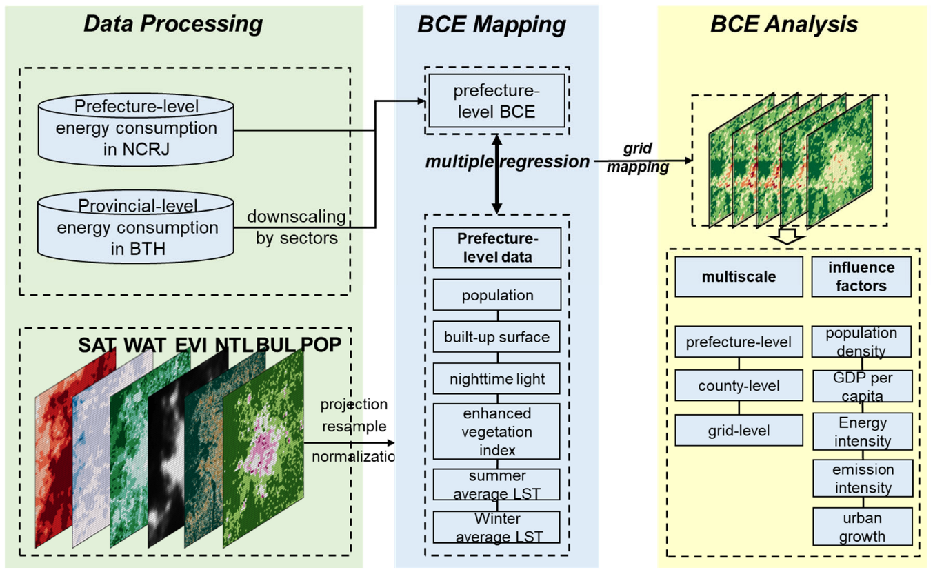
2.3. Estimation of Multi-Scale Emissions from Building Operations

Mapping BCEs at the grid scale involves integrating remote sensing and statistical data, analyzing spatial–temporal characteristics and influencing mechanisms of multi-scale BCEs. The research framework for this paper includes three parts (Figure 2). Data processing mainly focuses on preprocessing the calculation of prefecture-level BCEs and remote sensing data. Based on prefecture-level datasets, we used a multiple linear regression (MLR) model to build the relationship between prefecture-level BCEs and remote sensing data. The results were used to downscale prefecture-level BCEs to a grid scale. In the third part, an LMDI model was used to analyze the temporal and spatial characteristics of BCEs at different scales and determine the factors affecting changes in BCEs.

2.3.1. Calculation of BCEs at the Prefecture Level

In the operation stage, carbon emissions from energy consumption are mainly caused by living, commercial, and office activities. In this paper, we used the IPCC method to calculate building operation emissions at the provincial and prefecture levels using the BTH’s provincial energy consumption statistical data and the NCRJ’s prefecture-level energy consumption data.

$$CE=\sum _{i=1}{EC}_i\times {NCV}_i\times {CC}_i\times {COF}_i\times 44/12$$

(1)

where $CE$ refers to CO₂ emissions caused by energy consumption; and ${EC}_i$, ${NCV}_i$, ${CC}_i$, and ${COF}_i$ are the energy consumption, net calorific value, carbon content, and carbon oxide rate of $i$ type of energy. The energy consumption at the provincial level and the factors above of the BTH referred to China’s Energy Statistical Yearbook (https://data.cnki.net/) (accessed on 12 November 2022) We referenced the Agency for Natural Resources and Energy (https://www.enecho.meti.go.jp/) (accessed on 12 November 2022) and Ministry of the Environment (https://www.env.go.jp/en/) (accessed on 12 November 2022) for the NCRJ’s energy consumption at the provincial level and the factors shown above.

Considering the available data and estimation scales, the calculation of building operation emissions (BCEs) in this study relied on dividing building operations’ energy consumption from different sectors.

$${BCE}_1={BCE}_c+{BCE}_r+{BCE}_o+{BCE}_t$$

(2)

${BCE}_1$ is one part of BCEs, including emissions from the commercial and retail sector (${BCE}_c$), residential sector (${BCE}_r$), other sectors (${BCE}_o$), and transport sector (${BCE}_t$). Because energy balance sheets in the BTH and NCRJ record various levels of energy consumption by activity sectors, the energy consumption in commercial, residential, and other sectors also includes energy related to transport; the energy related to transport in the above sectors is removed to a certain extent. The specific proportion was referred to in previous studies [21,41]. For instance, 95% of gasoline consumption and 35% of diesel consumption in the commercial and retail sectors were removed, 95% of gasoline consumption and 35% of diesel consumption in other sectors were removed, and 95% of gasoline consumption and all diesel consumption in the residential sector were removed from the calculation. Since the transport stations and storage are public buildings and need energy to maintain operations, coal and 40% of electricity consumption were used to calculate the BCEs in transport stations, storage, and post-sector.

$${BCE}_2={BCE}_{cheating}-({BCE}_c^{heating}+{BCE}_r^{heating}+{BCE}_o^{heating})$$

(3)

${BCE}_2$ are the emissions caused by heating. To avoid double counting, the heat used by sectors in the energy balance sheet was removed, and heating emissions were calculated based on central heating supply statistics (${BCE}_{cheating}$). Since the central heating supply is concentrated in Northern China, Equation (3) applies to the BTH calculation. The emissions from heating in the NCRJ were calculated by the consumption levels of sectors using Equation (2).

$$BCE={BCE}_1+{BCE}_2$$

(4)

$BCE$ represents the total emissions from building operations of the region.

The prefecture-level statistics of sectors’ energy consumption in Hebei Province are limited. Therefore, the top-down decomposition method was adopted to obtain BCEs at the prefecture level in Hebei Province. The corresponding decomposition indicators are shown in

Table A1. Corresponding indicators for downscaling the BCE to prefecture level in Hebei province.

	BTH
Commercial and retails	Total retail sales of consumer goods
Residential	Electricity consumption for residential
Other	Gross domestic product of tertiary industry
Transport	Passenger traffic/Freight traffic/Number of public transportation vehicles and taxis/
Heating	Urban central heating

Appendix A.

2.3.2. Mapping BCEs at the Grid Scale by Integrating Remote Sensing Data and Statistical Results

As previous studies have proved that the economic output, population, and urban expansion have positive effects on buildings’ carbon emissions because of increasing demand for energy consumption [40,41,42], we selected nighttime light data, grid-scale population data, and built-up land data to represent the socioeconomic factors influencing BCEs. Summer and winter temperatures affect the building energy consumption required to maintain comfortable conditions [35,36,37]. Vegetation loss indirectly affects BCEs by intensifying the urban heat island effect and influencing the temperature around buildings [38,39]. Therefore, the summer mean temperature, winter mean temperature, and vegetation index were selected as natural factors in regression models. The remote sensing data were adjusted to a resolution of 1 km and Lambert conformal conic projection after preprocessing, normalized using Equation (5).

$${NX}_i=\frac{x_i-x_{min}}{x_{max}-x_{min}}$$

(5)

The BCEs of public buildings ($BCEP$) included emissions from the commercial and retail sectors, other sectors, and the transport sector. The BCEs of residential buildings ($BCER$) include emissions from the residential sector. The emissions from central heating were divided into public heating and residential heating using the proportion of heat in the BTH’s energy balance sheet. Equations (6) and (7) show the multiple linear regression (MLR) models for public and residential BCEs, respectively. ${NNTL}_i$, ${NPOP}_i$, ${NPBL}_i$, ${NRBL}_i$, ${NEVI}_i$, ${NST}_i$, and ${NWT}_i$ represent the nighttime light data, population, public built-up land, residential built-up land, enhanced vegetation index, summer temperature, and winter temperature after normalization, respectively.

$${BCEP}_i={\beta }_0+{\beta }_1{NNTL}_i+{\beta }_2{NPOP}_i+{\beta }_3{NPBL}_i+{\beta }_4{NEVI}_i+{\beta }_5{NST}_i+{\beta }_6{NWT}_i+{\epsilon }_i$$

(6)

$${BCER}_i={\beta }_0+{\beta }_1{NNTL}_i+{\beta }_2{NPOP}_i+{\beta }_3{NRBL}_i+{\beta }_4{NEVI}_i+{\beta }_5{NST}_i+{\beta }_6{NWT}_i+{\epsilon }_i$$

(7)

Based on the results of Equations (6) and (7), the models were applied to a 1 km grid. To obtain the final results of grid-scale emissions (${BCE}_g$), prefecture-level emissions were used to revise the estimation results.

$${BCE}_g=\frac{{BCEP}_g^{\prime }}{\sum _{g=1}{BCEP}_g^{\prime }}\times BCEP+\frac{{BCER}_g^{\prime }}{\sum _{g=1}{BCER}_g^{\prime }}\times BCER$$

(8)

2.3.3. Decomposition of Factors Affecting BCE Growth

According to the Kaya model, BCEs can be decomposed using Equation (9):

$$BCE=\frac{BEC}{EC}\times \frac{EC}{GDP}\times \frac{GDP}{P}\times \frac{P}{BL}\times BL$$

(9)

where $EC$, $GDP$, $P$, and $BL$ refer to the energy consumption (GJ), gross domestic product, population, and built-up land, respectively. The $\frac{BEC}{EC}$, $\frac{EC}{GDP}$, $\frac{GDP}{P}$, $\frac{P}{BL}$, and $BL$ represent the carbon emissions intensity (CEI), energy intensity (EI), GDP per capita (GP), population density (PD), and urban expansion (UE), respectively, which cover the economic, population, and built environment factors of regional growth.

The Logarithmic Mean Divisia index (LMDI) model is an extension of index decomposition analysis (IDA) and has been widely used in exploring driving factors in energy consumption, CO₂ emissions, and other social and ecological subjects [67,68]. The LMDI was applied to decompose the factors of BCE growth ($∆BCE$) in this study.

$$∆BCE={BCE}_t-{BCE}_0=∆CEI+∆EI+∆GP+∆PD+∆UE$$

(10)

${BCE}_t$ and ${BCE}_0$ represent BCEs in the year $t$ and base year $0$, respectively. According to the LMDI model, the $∆BCE$ was decomposed into $∆CEI$, $∆EI$, $∆GP$, $∆PD$, and $∆UE$. Since the growth rate of BCEs was defined as the relative growth of BCEs in the base year, the ${Grow}_{bce}$ may be transferred using Equation (11):

$${Grow}_{bce}=\frac{∆BCE}{{BCE}_0}=\frac{∆CEI+∆EI+∆GP+∆PD+∆UE}{{BCE}_0}$$

(11)

Therefore, the contributions of $∆CEI$, $∆EI$, $∆GP$, $∆PD$, and $∆UE$ to the growth rate of BCEs were calculated using Equations (12) to (16):

$$∆CEI=\frac{{BCE}^t-{BCE}^0}{{lnBCE}^t-{lnBCE}^0}ln\left(\frac{{CEI}^t}{{CEI}^0}\right)$$

(12)

$$∆EI=\frac{{BCE}^t-{BCE}^0}{{lnBCE}^t-{lnBCE}^0}ln\left(\frac{{EI}^t}{{EI}^0}\right)$$

(13)

$$∆GP=\frac{{BCE}^t-{BCE}^0}{{lnBCE}^t-{lnBCE}^0}ln\left(\frac{{GP}^t}{{GP}^0}\right)$$

(14)

$$∆PD=\frac{{BCE}^t-{BCE}^0}{{lnBCE}^t-{lnBCE}^0}ln\left(\frac{{PD}^t}{{PD}^0}\right)$$

(15)

$$∆UE=\frac{{BCE}^t-{BCE}^0}{{lnBCE}^t-{lnBCE}^0}ln\left(\frac{{UE}^t}{{UE}^0}\right)$$

(16)

3. Results

3.1. Results of MLR Models and Evaluation of Multi-Scale BCEs

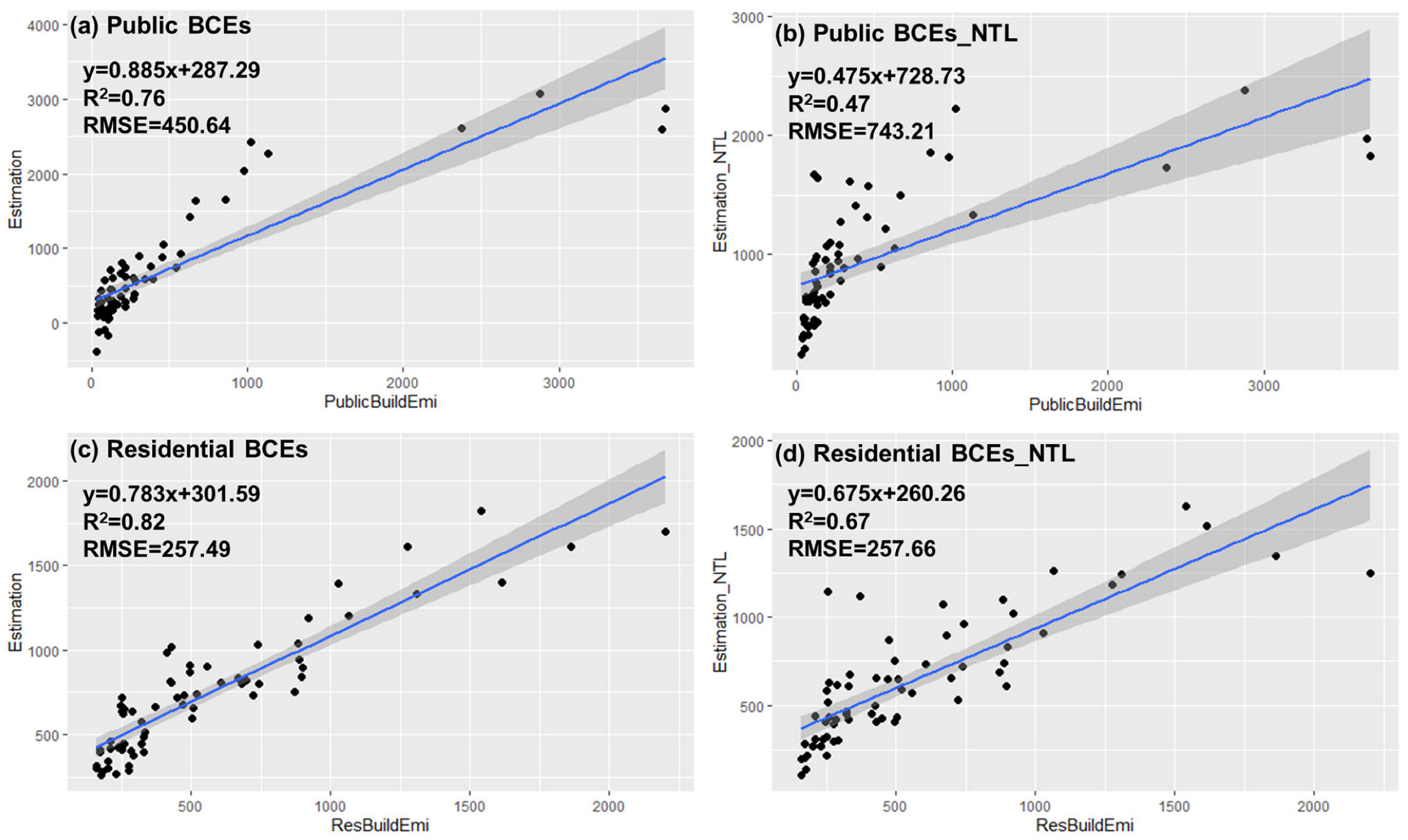
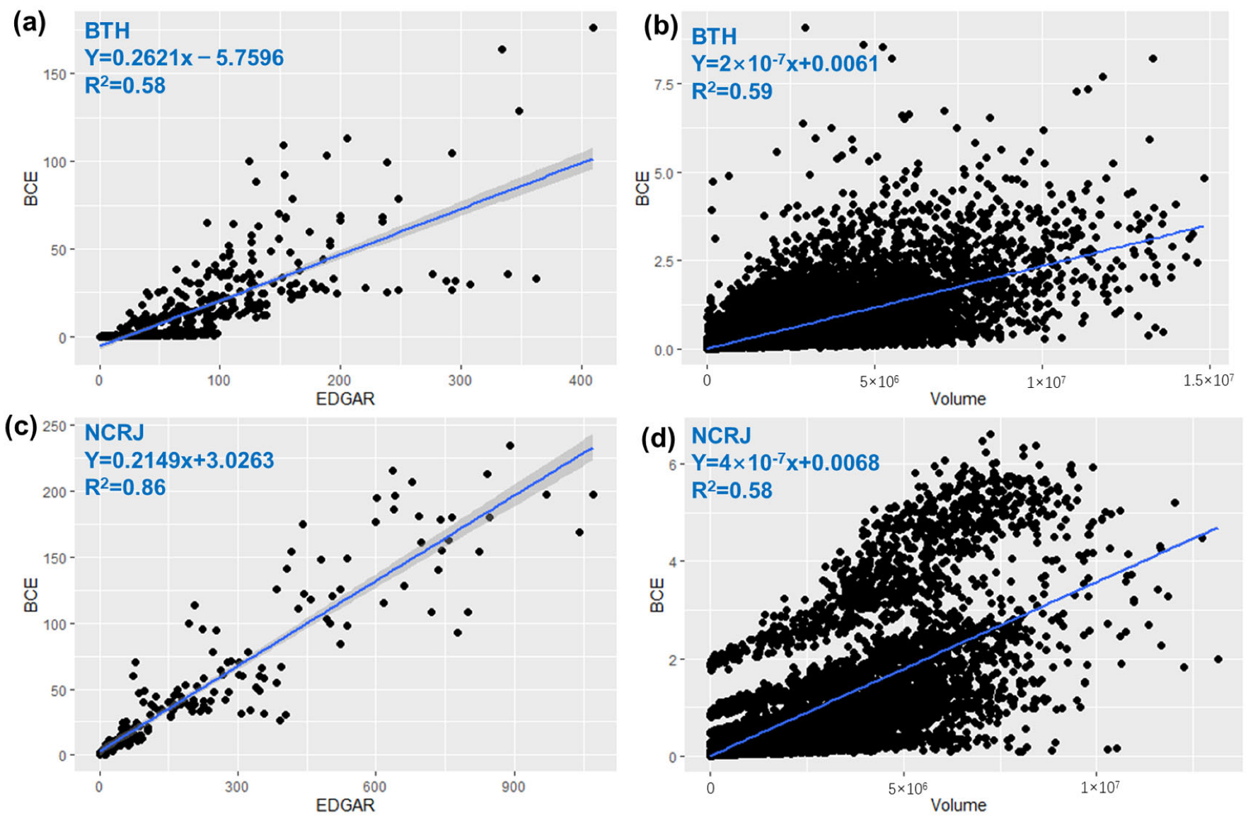
3.1.1. Results of MLR between BCE and Remote Sensing Data

Table 2. Results of regression between public BCEs and remote sensing data.

Variables	BTH	NCRJ
NTL	−0.059	−1.346 ***
POP	12.076 ***	1.893 ***
PLU	9.464 ***	−0.538 ***
EVI	0.027	0.167
ST	0.081 **	1.655 ***
WT	0.052 ***	−0.130
Observations	65	40
R2	0.79	0.97

*** p < 0.01, ** p < 0.05.

and

Table 3. Regression results between residential BCEs and remote sensing data.

Variables	BTH	NCRJ
NTL	0.094 **	−0.439 **
POP	8.740 ***	1.189 ***
RLU	0.159	−0.065
EVI	−0.009	−0.332 *
ST	−0.029	0.604 **
WT	0.028	0.097
Observations	65	40
R2	0.85	0.99

*** p < 0.01, ** p < 0.05, * p < 0.1.

show the multiple linear regression results for BCEs from public and residential buildings by remote sensing data, respectively. Table 1 shows that the population (POP), public built-up land (PLU), summer temperature (ST), and winter temperature (WT) results are effective. These factors positively affect public BCEs, indicating that the large population size, high proportion of public built-up land, and high temperatures in summer and winter cause higher levels of CO₂ to be produced in public building operations, which is consistent with the trend of higher energy demand in urban areas where socio-economic activities are concentrated. The NCRJ results showed that the nighttime light, population size, public built-up land, and summer temperature were effective. The BCEs of prefectures in the NCRJ have seen a downward trend in recent years, and increased factors, such as nighttime light and public built-up land, have adversely affected public BCEs.

Table 3 shows the regression results between residential BCEs and remote sensing data. The nighttime light and population size positively affect residential BCEs in the BTH. The NCRJ’s regression results showed that the nighttime light, population size, enhanced vegetation index (EVI), and summer temperature positively affect residential BCEs. In particular, the population size and summer temperature positively affect the residential BCEs, whereas nighttime light and enhanced vegetation index negatively affect residential BCEs. On the one hand, they have been affected by reduced emissions from residential buildings since 2015. On the other hand, due to a lower population density and social and economic activities, areas with a higher degree of vegetation consume relatively less energy.

Although the significant effect of vegetation cover on surface temperature and urban heat island which affecting buildings’ energy consumption indirectly are proposed from previous studies [38,39], the regression results of EVI did not show a significant impact on BCEs, especially in BTH urban agglomeration. We make a liner regression between EVI and BCEs (Figure A1). It can be found that results in BTH does not show significant correlation with BCEs but results in NCRJ show a relatively clear downtrend with EVI increasing, which is basically consistent with MLR models. In general, the results improved compared with the BCEs and NTL models (

Table A2. Regression results between BCEP and NTL.

	BTH	NCRJ
NTL	0.366 ***	−0.607
R-squared	0.475	0.039

*** p < 0.01.

and

Table A3. Regression results between BCER and NTL.

Title 1	Title 2	Title 3
NTL	0.250 ***	−0.277
R-squared	0.676	0.012

*** p < 0.01.

). To further explain the fitting results of study areas, we compared the prefecture-level estimation results with prefecture-level statistical BCEs. Figure A2 and Figure A3 show the comparison between the BTH and NCRJ, respectively. Figure A2a,c are the fitting results between estimation results using MLR and statistical results, showing almost consistent explanations for the estimations of public and residential BCEs with R², which are 0.76 and 0.82, respectively. Compared with the fitting results between estimation results using nighttime light data and statistical results (Figure A2b,d), estimation results using MLR are approaching the statistical results. Fitting results between prefecture-level estimation results and statistical results in the NCRJ also show consistency with Table 2, indicating the high explanation of statistical results to estimation results of public and residential BCEs with R2, which are 0.97 and 0.99, respectively (Figure A3).

Table 4. Models for downscaling BCEs in the BTH and NCRJ.

Variables	BTH	NCRJ
Public BCE	$BCEP=12.076\ast POP+9.464\ast PLU+0.081\ast ST+0.052\ast WT$	$BCEP=-1.346\ast NTL+1.893\ast POP-0.538\ast PLU+1.655\ast ST$
Residential BCE	$BCER=0.094\ast NTL+8.74\ast POP$	$BCER=-0.439\ast NTL+1.189\ast POP-0.332\ast EVI+0.604\ast ST$

lists the models for downscaling prefectures’ BCEP and BCER to a grid scale in the BTH and NCRJ based on Equations (6) and (7).

3.1.2. The Validity of Multi-Scale Estimation Results

Based on the regression results in Table 2, BCEs with a 1 km resolution can be calculated using effective factors of remote sensing data. To verify the results, the estimation results at the prefecture and county (municipality) levels in 2000, 2005, 2010, 2015, and 2019 were compared to emissions from the building sector provided by the Emissions Database for Global Atmospheric Research (EDGAR). EDGAR is a global database of the total CO₂ emissions and sector CO₂ emissions at an approximately 10 km ∗ 10 km resolution. The building sector’s CO₂ emissions from EDGAR focus on emissions caused by the combustion of fossil fuel at a country level, and the spatial proxies of it are fishing, the rural population, and urban population [69]. Although the accuracy of grid emissions from EDGAR’s building sector is affected by the population [70], it largely reflects the activity intensity of the building sector and, is appropriate for comparison with the estimated results in this study since the population is an important parameter in downscaling BCEs.

The fitting results at the prefecture level in the BTH showed that R² and RMSE were 0.81 and 11.91 million tons, respectively (Figure 3a). The R² and RMSE between estimation and EDGAR at the prefecture level in the NCRJ were 0.85 and 12.11 million tons, respectively, which were higher in the BTH (Figure 3c). Counties in the BTH and municipalities more than 100 square kilometers in the NCRJ were selected to verify the estimation results of BCEs at a finer scale. We found that the R² of county-level BCEs and EDGAR in the BTH urban agglomeration was 0.67, lower than that of the prefecture level, and the RMSE was about 0.95 million tons (Figure 3b). According to the fitting results, the R² and RMSE of the municipality level in the NCRJ were higher at 0.92 and 1.78 million tons, respectively (Figure 3d). The fitting results at different scales indicated that this study’s estimation results of BCEs are highly consistent with the scale trend in emissions from the building sector of the known database, among which the fitting effect of the NCRJ is better at a multi-scale. However, considering RMSE, the RMSE of the BTH urban agglomeration is lower.

Since the existing grid-scale BCE dataset with a 1 km resolution is limited, the grid-scale emissions of this study are resampled to a 10 km resolution to compare with EDGAR’s building sector (Figure A4a,c). Existing studies use other data related to building to verify their estimation results. Therefore, we compared grid-scale BCEs in 2019 with the grid-scale building volume in 2020, which is calculated using the building height in 2018 and built-up surface area in 2020 provided by the GHSL (Figure A4b,d). Although EDGAR’s building sector and building volume both show a linear correlation with the grid-scale estimation value of the BTH, the explanation for the fitting results is relatively lower compared with that at the prefecture and county levels, indicating the limitation of grid-scale estimation results in this study to a certain extent. Similarly, grid-scale fitting results in the NCRJ also show a significant linear correlation with EDGAR’s sector and building volume. However, the fitting results show a higher correlation between BCEs and EDGAR’s building sector, the R² of which is 0.86. In general, grid-scale estimation BCEs of this study have a relatively higher correlation with relevant building sector data, but the results of girds with similar volumes need to be further refined.

3.2. Spatial–Temporal Patterns of Multi-Scale BCEs

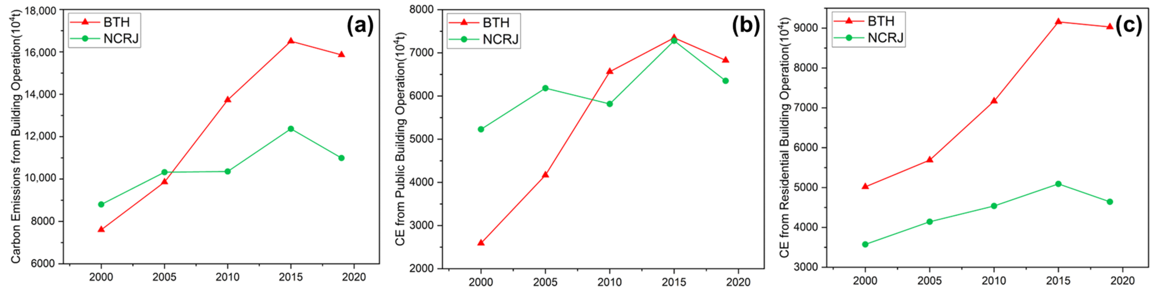
3.2.1. Total BCEs of the BTH and NCRJ

The BTH and NCRJ’s BCEs increased continuously from 2000 to 2015 and decreased from 2015 to 2019. The BTH’s BCEs increased from 76.07 million tons in 2000 to 158.57 million tons in 2019, peaking at 165.04 million tons in 2015. The average annual growth exceeds 4 million tons. The NCRJ’s total BCEs increased from 88.02 million tons in 2000 to 123.71 million tons in 2015, and then decreased to 109.93 million tons in 2019 (Figure 4a). With rapid economic development, the BTH’s BCEP increased rapidly from 25.9 million tons in 2000 to 73.5 million tons in 2015 and has remained above 60 million tons since 2010. Although the NCRJ’s BCEP also maintains a fluctuating upward trend, the overall growth scale and speed are lower than that of the BTH and show a significant downward trend from 2015 to 2019 (Figure 4b). Since the total population and built-up land of the BTH are higher than those of the NCRJ, the BTH’s BCER is higher than the NCRJ’s BCER and increased rapidly since 2005 from nearly 50.17 million tons to 91.56 million tons. The growth speed of the NCRJ’s BCER is slower, which increased from 35.73 million tons to 50.91 million tons and then dropped to 46.42 million tons in 2019 (Figure 4c). In general, the BTH’s BCEs maintained a trend of rapid and large-scale growth since 2000, while the NCRJ’s BCEs showed a fluctuant and small growth trend.

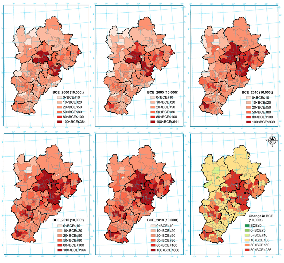
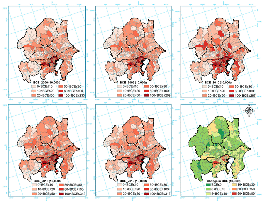
3.2.2. Prefecture-Level BCEs

There are significant differences in scale and changes between prefecture cities in the BTH (Figure 5). Although Beijing’s BCEs are the highest in the BTH compared with other prefectural cities, Beijing is the first city in the region to show a downward trend between 2015 and 2019. The BCEs in Beijing increased from 21.57 million tons in 2000 to 58.85 million tons in 2015, and fell to 44.14 million tons in 2019. Other prefecture cities in the BTH maintained a trend of growth in BCEs from 2000 to 2019. Tianjin, Shijiazhuang, Tangshan, Baoding, and Handan showed relatively high growth in BCEs. Tianjin’s BCEs increased from 13.69 million tons in 2000 to 26.36 million tons in 2019. Shijiazhuang, Tangshan, Baoding, and Handan’s BCEs exceeded 10 million tons in 2019, about twice the emissions in 2000. Cangzhou, Xingtai, Langfang, and Zhangjiakou’s BCEs exceeded 5 million tons in 2019. Hengshui, Qinhuangdao, and Chengde’s BCEs exceeded 3.5 million tons in 2019. Overall, the decrease in the BTH’s BCEs in 2019 is mainly attributed to the decrease in Beijing’s BCEs, while emissions of the other 12 prefecture cities in the region maintained a growth trend and most prefecture cities experienced their highest increase in emissions from 2010 to 2015.

The emissions of all prefectures in the NCRJ showed significant downward trends during the study period, which is different from the increased trend in the BTH (Figure 6). Tokyo’s BCEs reached 48 million tons in 2015 and then dropped to 43.56 million tons in 2019. Kanagawa, Saitama, and Chiba’s BCEs maintained more than 10 million tons from 2000 to 2019, and Kanagawa’s BCEs exceeded 20 million tons from 2015. However, Ibaraki, Tochigi, Gunma, and Yamanashi’s BCEs were relatively lower since they are further away from Tokyo. The first decline appears between 2005 and 2010, shown as a slight decreasing trend. A significant decline in BECs between 2015 and 2019 shows that Tokyo and Saitama Prefecture’s BECs decreased by 4.45 and 3.27 million tons in 2019, respectively. The decreases in Kanagawa, Chiba, and Ibaraki prefectures’ BCEs exceeded 1 million tons. On the whole, the change trend of prefectures in the NCRJ is consistent, and a significant emission reduction has occurred in recent years.

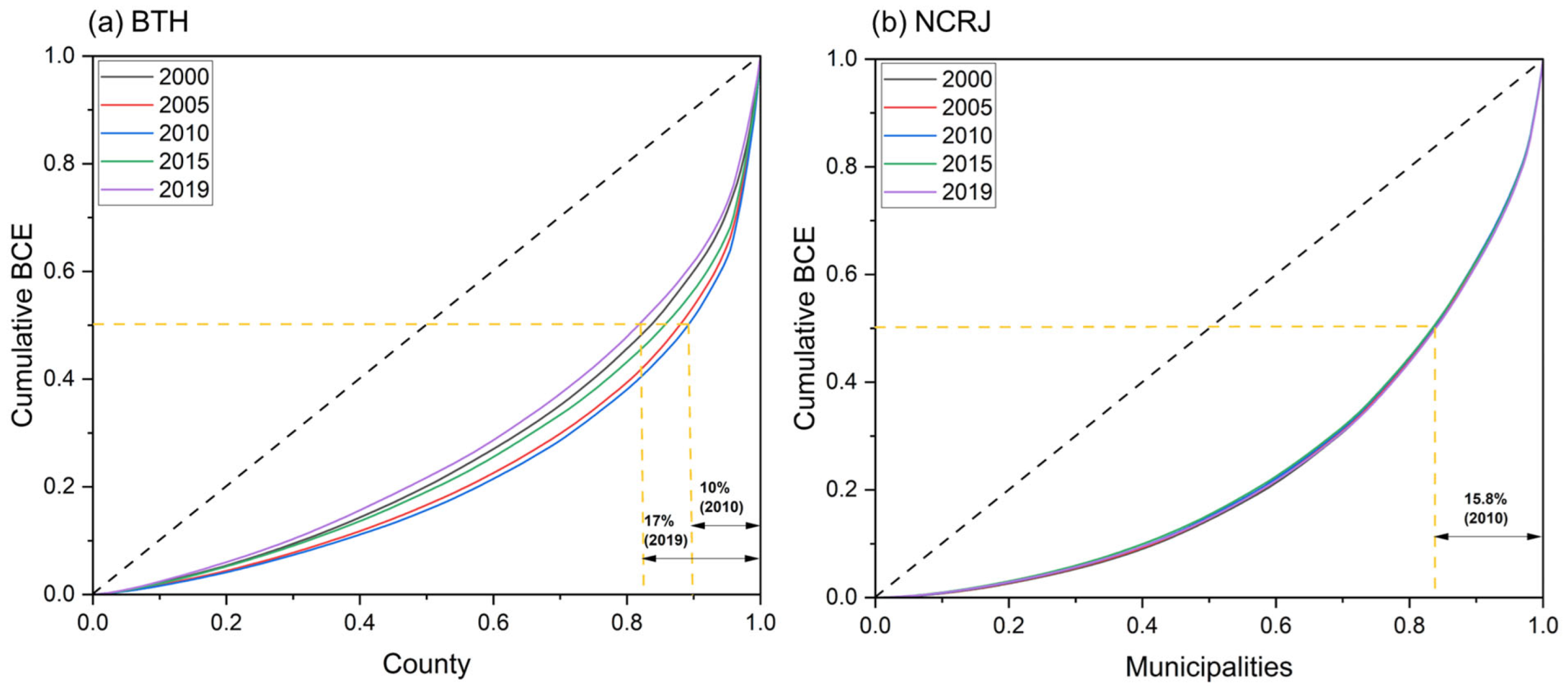
3.2.3. County-Level BCEs in the BTH and Municipality-Level BCEs in the NCRJ

According to the Lorentz curve of county-level emissions of the BTH, the curves deviate from the mean line, showing significant scale differences in BCEs between counties in the BTH (Figure 7a). The degree of curve deviating from the mean line increases continuously from 2000 to 2010, indicating that scale differences between counties’ BCEs increase due to high-emission counties’ growth rate being faster than middle- and low-emission counties. However, with the acceleration of the growth of middle- and low-emission counties’ BCEs, the differences in the BCE scale between counties are reduced and the curves of 2015 and 2019 are relatively approaching the mean line. Similarly, 10% of counties’ BCEs accounted for 50% of the total BCEs in 2010, and this proportion increased to 17% in 2019.

The Lorentz curves of municipalities’ BCEs in the NCRJ also deviate far from the mean line, but the multi-year curves almost overlap, which means that there are significant differences in the scale between municipalities’ BCEs but the differences remain stable and show barely interannual changes (Figure 7b). Since the municipalities’ BCEs maintain similar growth and decline rates, the proportion of high-emission municipalities accounting for 50% of the total BCEs was about 15.8% from 2000 to 2019.

From the perspective of spatial patterns, there are significant interannual changes in BCEs at the county level within the BTH (Figure 8). The BCE of most counties exceeded 200,000 tons in 2000. Chaoyang, Haidian, Fengtai, Changping, Shunyi, Tongzhou, Daxing, and Fangshan in Beijing and Dongli, Beichen, Xiqing, and Binhai New District in Tianjin’s BCEs exceeded 1 million tons, forming a significant high-emission cluster. With the emissions of the BTH increasing rapidly between 2005 and 2010, the number of counties generating more than 1 million tons in Beijing and Tianjin increased significantly. In addition, counties’ BCEs in Tangshan, Shijiazhuang, and Handan also continued to increase. For example, the BEC of Fengrun and Qianan in Tangshan, and Wuan in Handan exceeded 1 million tons. The number of counties with BECs over 200,000 tons in Chengde and Langfang also increased. The BEC of most counties in the BTH still maintained a significant growth trend from 2010 to 2015, and the main patterns include the concentration of high-emission counties in Beijing and Tianjin, the distribution of counties with emissions higher than 1 million tons in Shijiazhuang and Baoding, and the increase in the number of counties with emissions exceeding 500,000 tons in Shijiazhuang, Baoding, Cangzhou, and Handan. Compared with the previous period, the number of counties with high emissions increased in Tianjin, Shijiazhuang, and Tangshan in 2019. In general, counties’ BCEs in the BTH observably increased from 2000 to 2019. Due to the rapid speed of development with a relatively large population size and dense buildings, the change in BECs of counties surrounding core areas in Beijing, Tianjin, Shijiazhuang, and Tangshan exceeded 500,000 tons.

Municipalities’ BCEs in the NCRJ are more stable and vary within a smaller range (Figure 9). Most municipalities’ BCEs reached 100,000 tons, and the emissions of most municipalities in Tokyo, Kanagawa, Saitama, and Chiba prefectures exceeded 200,000 tons. Most of the high-emission municipalities with emissions above 1 million tons are concentrated in Tokyo including Hachioji, Machida, Shinjuku, Koto, Ota, Setagaya, and other areas located on the fringes of the special ward. The changes in most municipalities’ BCEs in the NCRJ were less than 50,000 tons, but the changes in BECs of parts of municipalities in Ibaraki, Saitama, and Chiba were between 50,000 tons and 100,000 tons. Changes in municipalities’ BCEs in Tokyo, Kanagawa, and southern Chiba exceeded 100,000 tons. Areas with changes exceeding 300,000 tons mainly included Hachioji, Machida, and the fringes of the Tokyo special wards, which are consistent with the high-emission areas.

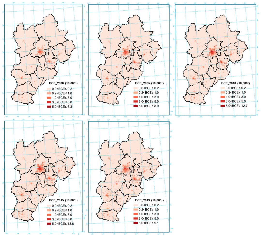
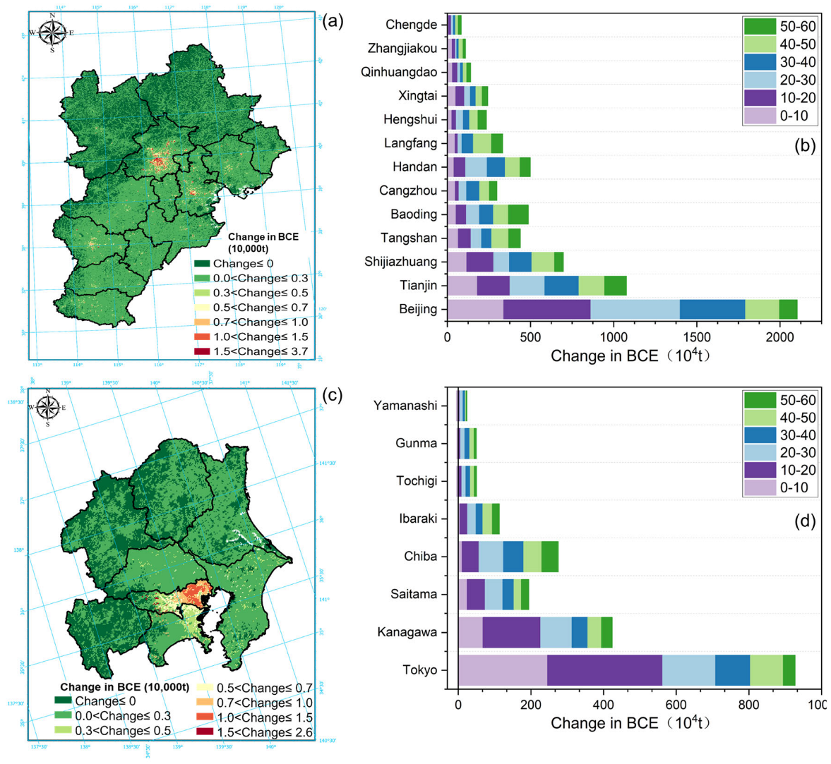
3.2.4. Spatial Pattern of and Change in BCEs at the Grid Scale

High-emission grids are mainly concentrated in core areas of cities in the BTH, and the number of grids with emissions exceeding 30,000 tons per km² continued to grow during the study period. The high-emission grid spreads to the periphery of core areas (Figure A5). The grids with more than 30,000 tons in the NCRJ are mainly concentrated in the special wards of Tokyo. The grids with emissions between 10,000 tons and 30,000 tons are mainly found in the midland of Tokyo and eastern Kanagawa. In general, the high-emission areas in the NCRJ are more concentrated and the highest emissions at the grid scale are lower than those of the BTH (Figure A6).

Except for the mountainous areas in the northwest of the BTH, most areas show positive growth in BCEs compared with 2000 (Figure 10a). The grids with more than 3000 tons of BCEs are concentrated in the urban areas of Beijing, Tianjin, and Shijiazhuang. The high-emission growth in Beijing forms a continuous distribution pattern with a large area and much of those show changes in emissions exceeding 10,000 tons. The growth in BCEs in other cities is mostly scattered across urban areas or the surrounding towns. The position of the prefectural government provided by RESD and MLIT is defined as the urban center of prefecture-level areas, and buffer statistics for each 10 km range are conducted based on the center to analyze the growth of BCEs with the distance range (Figure 10b,d). The BCEs’ total growth in Beijing, Tianjin, and Shijiazhuang within 60 km was 21.03, 10.77, and 6.98 million tons, respectively. The BCEs’ growth within 30 km in most cities accounted for 50% or more of BCEs’ total growth in the city. For the cities with relatively high economic development represented by Beijing, Tianjin, Shijiazhuang, and Tangshan, since the development of urban areas and surrounding suburbs are relatively parallel, there are not very large differences in BCEs’ growth within 0–10 km, 10–20 km, and 20–30 km of the city; for instance, the BCEs’ growth within 0–10 km, 10–20 km, and 20–30 km in Tianjin is 1.8 million tons, 1.96 million tons, and 2.09 million tons, respectively. Due to the development of towns around the urban areas in Baoding, Handan, Cangzhou, and Langfang, the growth outside the 20 km range accounts for a higher proportion of the total growth.

The grids with a BCE growth exceeding 7000 tons in the NCRJ are mainly situated in Tokyo, and grids in most special wards around Chiyoda increased by more than 10,000 tons (Figure 10c). Besides the grids in eastern Kanagawa showing an increase in BCEs between 3000 and 7000 tons, the growth of other grids’ BCEs was mostly less than 3000 tons across the study period. A significant difference in BCE change between Tokyo and other prefectures was caused by larger changes in the BCEs and downscaling factors of Tokyo. Tokyo shows relatively intensive regional development and sustained population attraction compared with other prefectures. In summary, the obvious changes are more concentrated in Tokyo and Kanagawa. Comparing the growth of BCEs within the corresponding distance, it is found that the growth of BCEs within 10–20 km in most prefectures accounts for the highest proportion of total BCE growth due to the larger area and similar scales of population, built environment, and economic activity with core areas (Figure 10d).

3.3. Decomposition of Influencing Factors for BCE Growth

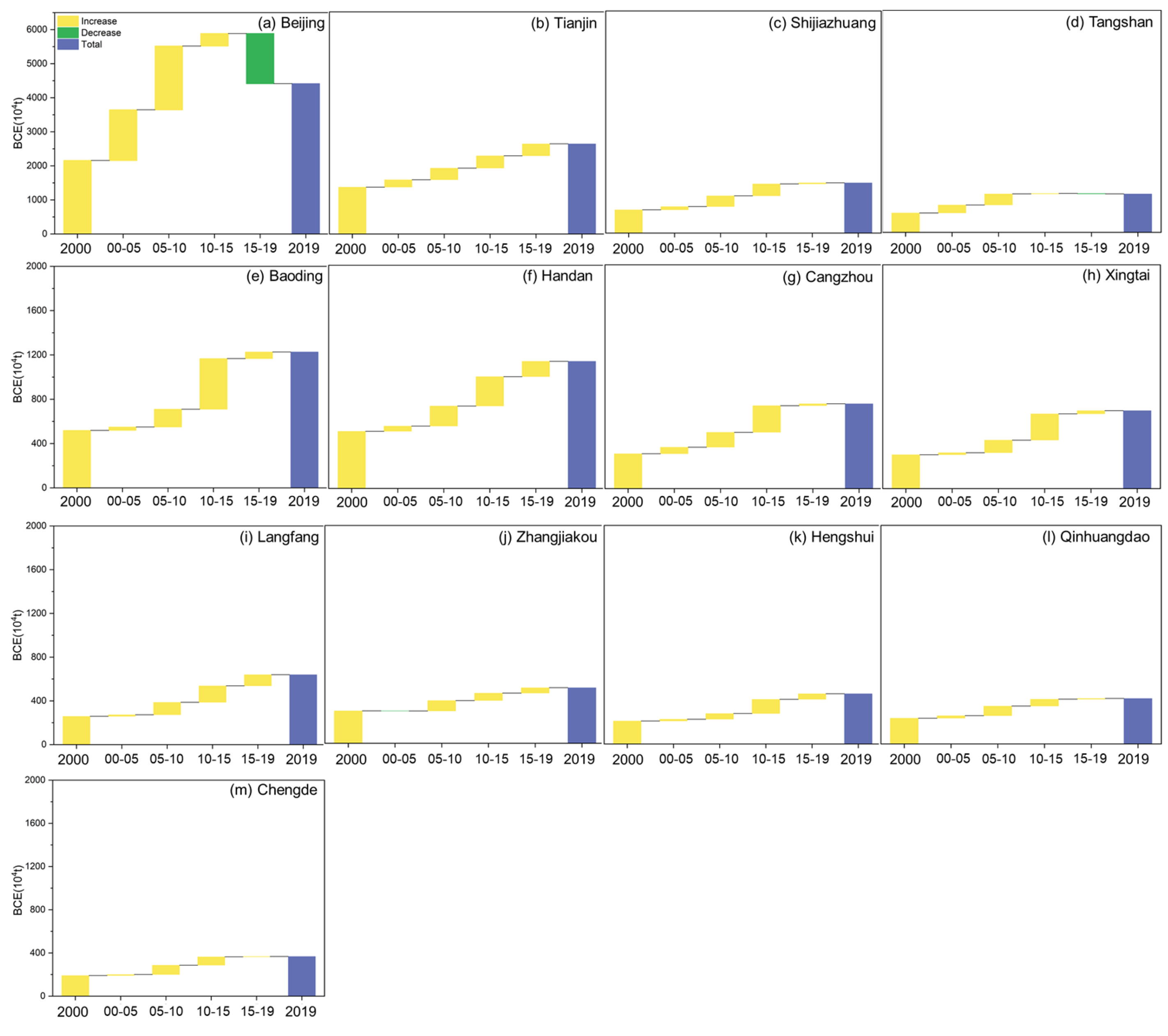
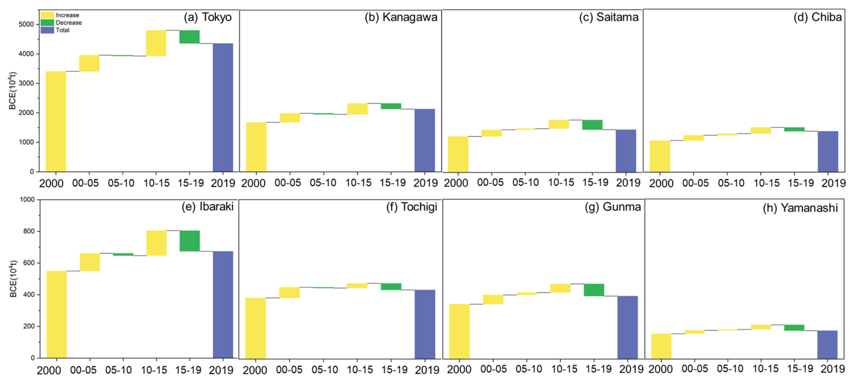
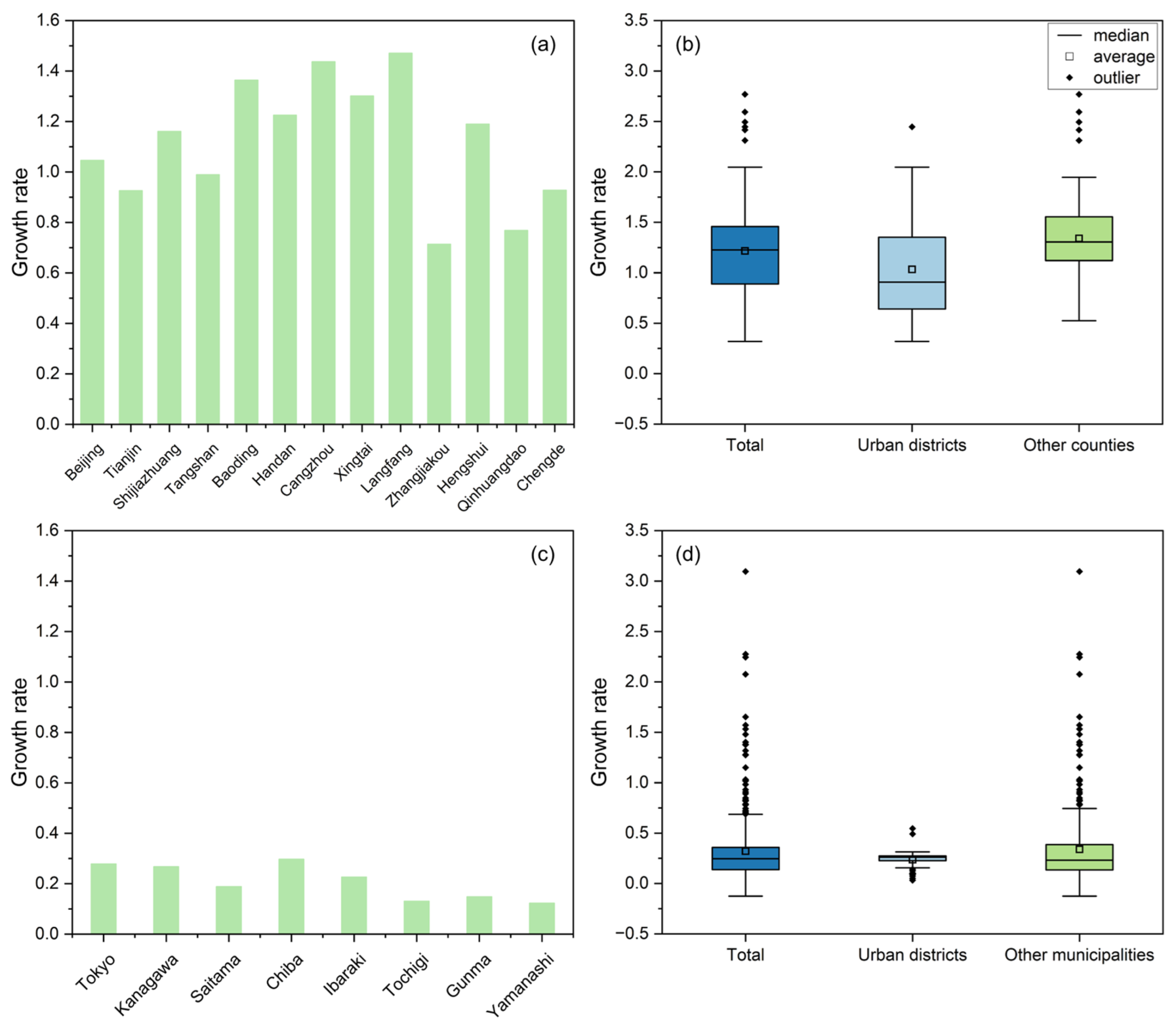
3.3.1. Characteristics of BCE Growth

By comparing the growth rates of BCEs at different scales between the BTH and NCRJ, we found that the growth rates of BCEs in the BTH were higher than those in the NCRJ. The growth rate of BCEs in all BTH cities was >0.6 from 2000 to 2019, among which Langfang had the highest rate at 1.47, followed by Cangzhou with 1.43. Zhangjiakou and Qinhuangdao City had lower growth rates of 0.71 and 0.76, respectively, and the BCE growth rates in other cities were >0.9 (Figure 11a). By contrast, the BCE growth rates in the NCRJ prefectures were <0.4, and the differences between prefectures were minor, particularly in Chiba, Tokyo, Kanagawa, and Ibaraki, which were relatively high at >0.2 (Figure 11c). The average growth rates of all counties, urban areas, and other BTH counties were 1.21, 1.03, and 1.34, respectively (Figure 11b), which were higher than the municipalities (0.32), urban areas (0.23), and other municipalities (0.33) in the NCRJ (Figure 11d). In addition, the growth rates in 50% of the BTH counties ranged from 0.8 to 1.4, whereas the growth rates of 50% of municipalities in the NCRJ ranged from 0.12 to 0.35. Urban areas and other counties in the BTH had higher growth rates than urban areas and other municipalities in the NCRJ. However, the growth rates of BCEs in urban areas were relatively low, indicating that suburban development and population growth accelerated the growth of BCEs around urban areas. This feature was more significant due to the rapid urbanization of the BTH during the study period.

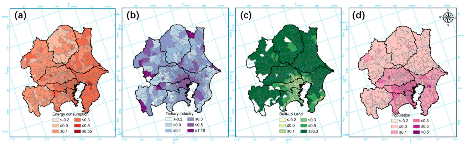
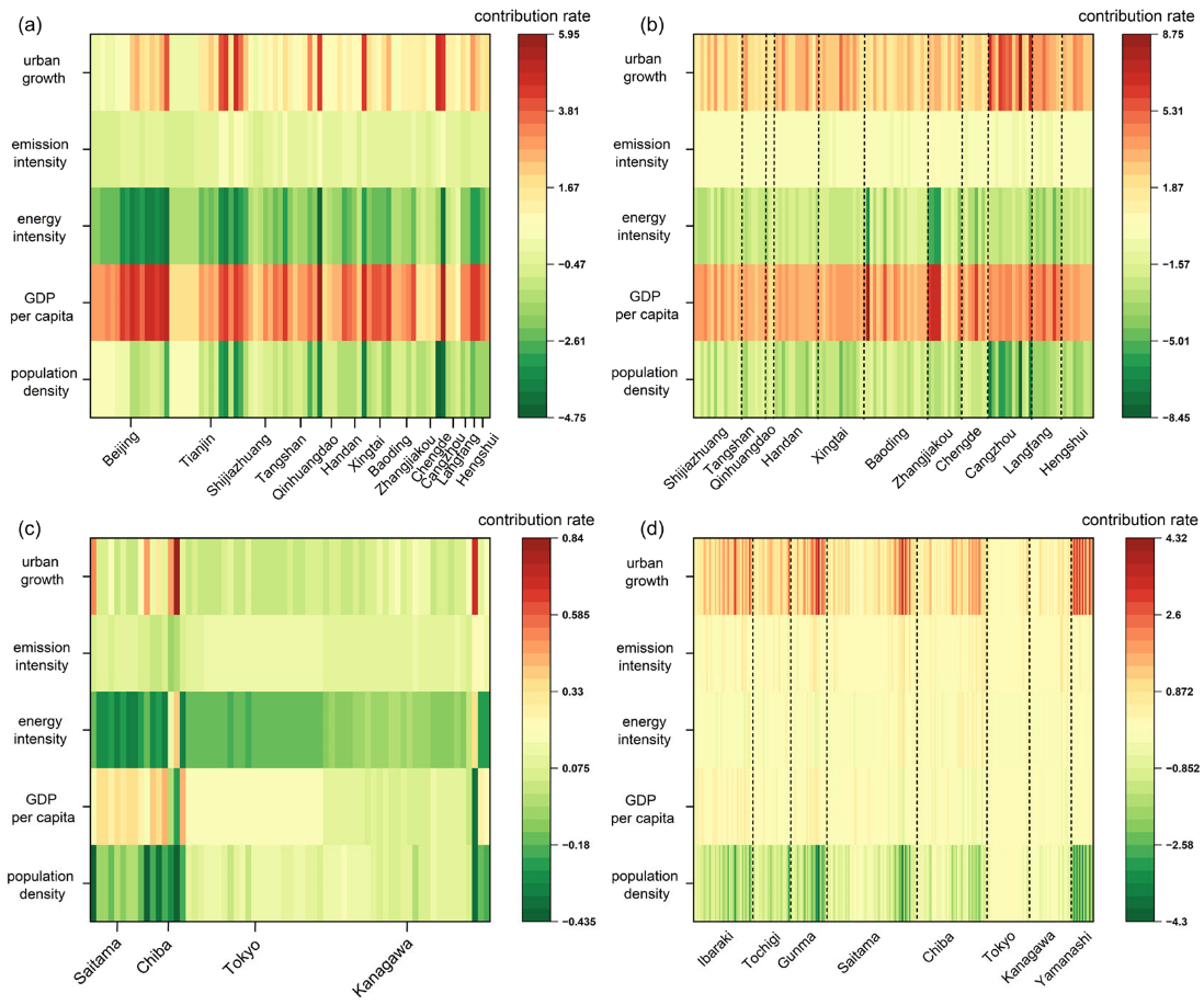
3.3.2. Decomposition of Influencing Factors at a Multi-Scale

From the perspective of prefecture-level growth in socioeconomic activities, the growth of the tertiary industry is significantly higher than the energy consumption, built-up land, and population, indicating the strong driving effect of consumption. Except for Beijing, the built-up land growth is higher than the population growth in other prefectures, which is an important driving factor following the tertiary industry. It is worth noting that the population in most prefectures has barely increased, which indicates potential land spread and inefficient use (Figure A7a). Based on the decomposition of influencing factors on BCE growth in the BTH, the growth of GDP per capita and built-up land significantly and positively contribute to the growth of BCEs, among which the contribution rate of GDP per capita is above 2.5, which is higher than the growth of built-up land (Figure 12a). These findings are consistent with urban growth and also indicate that economic development and urban expansion significantly increase building operations’ energy consumption and carbon emissions. By contrast, the population density, energy intensity, and emission intensity negatively contribute to the growth of BCEs. Reducing the energy intensity involves improving energy efficiency and technology and reducing the energy required per unit of economic output. Due to a nearly 80% decline in energy intensity between 2000 and 2019, BTH cities demonstrate the greatest negative contribution to BCEs, below −1.5. At the same time, decreased emissions per GJ and population per 1 km² of built-up land also negatively impacted changes in BCEs.

Prefecture-level growth in the energy consumption, tertiary industry, built-up land, and population in the NCRJ show patterns with significantly lower growth rates compared with the BTH. Built-up land is the major growth factor in prefectures during the stable development stage of the NCRJ. Meanwhile, except for the positive growth of the tertiary structure and population in Tokyo and Kanagawa, the growth of the population and economy in other prefectures is rare or even negative (Figure A7b). Decomposition results of factors influencing the growth of BCEs also show a consistent effect with urban growth. Compared to the BTH, the NCRJ’s positive and negative contribution rates have a lower absolute value due to the stable economic development, population, and urban scale of its prefectures (Figure 12b). The population density and energy intensity contribute negatively to changes in the BCEs of prefectures. In particular, the negative impact of the reduction in population density is noticeable, which is caused by population outflow and low birth rates. The increase in built-up land positively contributes to the growth of BCEs, which is higher than the GDP per capita and emission intensity in most prefectures. Similarly, existing studies also revealed the positive effect of urban land expansion on BCEs due to tertiary development [71].

County-level factors also show high growth in the tertiary industry and built-up land. The tertiary industry’s growth in most counties is above 10. Counties with high growth in built-up land are concentrated around core urban areas. Combined with the tertiary industry and population growth, it can be inferred that urban areas and suburban areas have experienced rapid development (Figure A8). The decomposition results of influencing factors at the county and municipality levels are divided into urban and other areas. For the county results in the BTH, the GDP per capita and built-up land expansion positively contribute to urban and suburban areas in the BTH. Conversely, the population density, energy intensity, and emission intensity are the main negative contributing factors (Figure 13a,b). In suburbs, however, the average contribution rates of GDP per capita and built-up land expansion are 3.81 and 2.92, respectively (Figure 13b), which are higher than core urban areas with 3.17 and 1.46 (Figure 13a). Similarly, the population density and energy intensity have a greater negative impact in the suburbs than in urban areas.

Municipality-level growth in energy consumption, tertiary industry, built-up land, and population are lower than in the BTH. Municipalities in Tokyo and Kanagawa show relatively rapid growth in the tertiary industry and population and weak growth in built-up land, indicating the activity intensity per unit area increased in core urban areas of the NCRJ (Figure A9). The decomposition results show that the contribution rates ranged from −0.435 to 0.84, and the variation range was significantly smaller than that of the BTH’s urban areas (Figure 13c). According to the decomposition results for influencing factors, the reduced energy required for economic output was the main negative contributing factor. Due to their close geographical location and the high and relatively stable development of Tokyo’s special wards, Yokohama and Kawasaki, the absolute value of positive and negative contribution rates of the municipalities were generally lower than those in Saitama, Chiba, and Sagamihara. In addition, the population density negatively impacted municipalities in Saitama, Chiba, and Sagamihara. The population density was the main negative contribution factor for other municipalities outside the main urban areas (Figure 13d). By contrast, the GDP per capita, energy intensity, emission intensity, and built-up land expansion positively contributed to most municipalities’ BCEs. The effect of built-up land expansion was also relatively high. Our results revealed that most municipalities have been facing a decline in population density due to low birth rates or population outflows. Under stable economic growth, land development and utilization have become the main source of BCE growth. However, for core areas in Tokyo and Kanagawa, the population inflow positively contributed to the population density of BCEs.

4. Discussion

The main contributions of this study could be summarized as three points. First, the study aims to mapping long-term BCEs combined remote sensing dataset and statistical energy consumption of building sector. Then, we explored the validity and improvement of MLR models compared with results obtained by nighttime light data along. Third, the mapping and analysis of BCEs are applied in BTH and NCRJ, which provides the differences in models’ validity and multi-scale BCEs between two regions. The discussion part mainly evaluates estimation results, effect of urban growth on BCEs, and limitations of this study.

4.1. Evaluation of Method for Estimating BCEs

This study explored the effectiveness of multi-dimensional remote sensing data in estimating emissions from building operations in the BTH and NCRJ. Multi-scale BCEs showed high consistency with existing databases in terms of the scale trend. However, similar trends do not mean fewer differences in specific emission scales. Figure A4 shows the differences between estimation results and statistical results of public and residential BCEs in the BTH and NCRJ. It can be found that the estimation results of the high-emission prefectures are similar to the statistical results, but there is an overestimation of the prefectures with emissions below 10 million tons (Figure A10a–c). However, differences between the estimated residential BCEs and statistical residential BCEs in the NCRJ are significantly smaller (Figure A10d), which is consistent with the small RMSE in Figure A3b. Although there are differences in the emission scale between estimation results and statistical results, the results after correction using statistical results are practicable because of a similar trend between them.

Although existing studies have confirmed the effectiveness of nighttime light data in estimating greenhouse gas emissions at different scales [64,72,73], the MLR model’s accuracy was improved by adding other factors. Moreover, factors related to sector activities should be considered when estimating sectors’ CO₂ emissions based on nighttime light data [26]. However, the effect of vegetation index on BCEs was not significant as expected. On the one hand, the results indicate the effect of EVI on BCEs is different among regions. On the other hand, the limited samples could not explain the appropriate relationship between vegetation and BCEs. For the improvement approaches, existing studies made regressions by groups which were divided by climate zones, natural conditions, and economic conditions [22,61]. Moreover, the data of vegetation dynamics could be considered using alternative dataset, such as gross primary production (GPP) and net primary production (NPP). GPP and NPP are defined as the energy captured per unit area per unit time through the process of vegetation photosynthesis and the energy after subtracting plant respiratory costs from GPP, respectively [74]. Both of them are important parameters for carbon cycle since the consideration of the production of biomass or carbon in ecosystem [74,75,76] and existing studies have explored the performances of vegetation indices in estimating GPP and NPP [77,78,79]. In addition, previous studies also combined the NPP and economic factors to calculate carbon footprint pressure and analyze the driving factors of carbon intensity [80,81,82]. From the direct relationship with vegetation cover, GPP and NPP are alternative to be used to analyze the influencing factors of BCEs.

Given the limitation of seasonal statistical data on the energy consumption of buildings, the estimations of BCEs at a multi-scale in this study are calculated by year. However, emissions from central heating account for a high proportion of prefecture-level BCEs in the BTH, indicating the high demand of energy in summer and winter (Figure A11). In addition, the differences in proportion between prefectures revealed the different patterns of heating supply between areas with large-scale urban populations and areas with large-scale rural populations. Therefore, analysis by seasons and urban–rural regions is essential for collecting finer statistical data and remote sensing data.

4.2. Implications of Urban Growth and Changes in BCE

The growth rate of BCEs at a multi-scale level in the NCRJ was relatively low despite its high-level and stable development. The differences in BCE growth rate between prefectures were also minor. Therefore, the prefectures within the NCRJ showed the same trend in BCEs during the study period and began to decline after 2015. By contrast, the overall growth rate of the BTH was relatively high. Due to rapid development and greater differences within the BTH urban agglomeration, the trend in BCEs was inconsistent in prefectures. For instance, Beijing showed a decline in BCEs after 2015, whereas the BCEs of most cities in Hebei Province continued to grow. From the perspective of urban growth, prefecture populations in the BTH urban agglomeration have increased significantly, with the growth rate exceeding 10%, namely in Tianjin (59%) and Beijing (68%). By contrast, Tokyo, Kanagawa, Saitama, and Chiba showed positive population growth, whereas other prefectures within the region had a negative growth rate during the study period. In terms of urban expansion, although the growth rates of built-up land in the BTH and NCRJ were higher than the population growth rate, the growth rates of built-up land in Beijing, Tianjin, Shijiazhuang, Tokyo, and Kanagawa were relatively low. They showed fewer differences than the population growth rate. However, the growth rates of built-up land in other prefectures were much higher than the population growth rate.

We found that population growth and built-up land expansion were important drivers for BCE growth during the rapid development stage. However, the positive effects of population growth and built-up land decreased during the stable development stage. The positive effect of built-up land expansion was higher than the population growth, according to the NCRJ’s results. For developed regions, the increase in emission intensity per unit area is the driving force behind BCE growth under the net population growth and urban sprawl control during the stable development stage [54]. These findings are similar to those of higher energy consumption and emissions per capita caused by low-density suburban development, higher energy consumption, and emissions per square meter in high-density core areas [83,84]. Urban growth impacts on BCEs are related to population increase, economic structure, and urban expansion [43]. The green innovation of commercial and public buildings for economic development is stressed along with the positive contribution of GDP per capita [85,86]. The positive contribution of urban expansion to BCEs also encourages compact urban planning and the rational allocation of land resources to support development demand [87]. Considering economic growth, reducing energy intensity negatively affected BCE growth in the BTH and NCRJ, underlining the need to optimize the industrial structure and improve the proportion of clean energy [88].

4.3. Limitations

As proposed in previous studies, the remote sensing data used for downscaling mainly included factors that impact BCEs. However, data directly related to buildings were not considered in the regression model due to data availability. We used prefecture-level nighttime light data as one factor to estimate the BCEs. This is a useful metric because nighttime light data not only reflects the intensity of public and residential buildings’ activities but also includes light from roads and vehicles. Therefore, the grid-scale emissions in the BTH may be slightly underestimated. To improve the results using nighttime light data, distinguishing urban and rural areas before estimating and processing nighttime light data to remove the light that is not included in the estimation scope is recommended. In addition, there was no comparison between the results of the MLR model used in this study and the machine learning or Cubist model used in previous studies. Due to the focus on socioeconomic factors in the analysis of BCE growth, the impact of natural factors was not included. Moreover, specific energy consumption comparisons and the policy-making influence were not considered in the analysis of socioeconomic factors.

5. Conclusions

This study focused on the downscaling of BCEs using integrating multi-source remote sensing data and the influence factors of BCE growth. The BTH urban agglomeration and the NCRJ were selected as the study areas. The prefecture-level BCEs in 2000, 2005, 2010, 2015, and 2019 were calculated using statistical data. The MLR model was constructed between prefecture-level BCEs and remote sensing data including the nighttime light, population, temperature, enhanced vegetation index, and built-up land to downscale BCEs to grid scale on a 1 km resolution in the BTH and NCRJ. Compared with the downscaling method using nighttime light data alone, adding other factors effectively improved the downscaling results. The R² (coefficient of determination) of fitting results between prefecture-level BCEs and EDGAR in the BTH and NCRJ are both above 0.8. The R² of county-level fitting results in the BTH and municipality-level fitting results in the NCRJ are 0.67 and 0.92, respectively. In general, the multi-scale estimation results in this study presented relatively high accuracy.

The BCEs of the BTH urban agglomeration increased from 76.07 million tons to 158.57 million tons from 2000 to 2019. The increases in BCEs at the prefecture, county, and grid levels are obvious. The emission scale of Beijing was the highest in the region and showed a downward trend between 2015 and 2019. Other cities in the BTH maintained an increasing trend during the study period. From the perspective of the spatial distribution, high-emission areas were concentrated in Beijing, Tianjin, and Tangshan. The total BCEs of the NCRJ increased slowly and dropped from a peak of 123.71 million tons in 2015 to 109.93 million tons in 2019. The BCEs at the prefecture level, municipality level, and grid level showed a significant downward trend between 2015 and 2019. The most high-emission areas were concentrated in Tokyo.

An LMDI model was used to decompose the influencing factors of BCE growth. It was found that the decrease in energy intensity and population density are the main negative factors, and the growth of GDP per capita and urban expansion significantly promote the growth rate of BCEs. Due to the rapid development of the BTH urban agglomeration, the intensity of positive or negative effects of influencing factors is higher than that of the NCRJ. This study attempted to verify the feasibility and accuracy of downscaling BCEs using multi-source remote sensing data in different regions. Based on the multi-scale emission analysis and the decomposition of influencing factors in study areas, the regional emission characteristics in different development stages are highlighted to provide a reference for the rapidly developing BTH urban agglomeration from the perspective of urban growth.

References

1. United Nations. World Urbanization Prospects: The 2018 Revision; United Nations, Department of Economic and Social Affairs, Population Division: New York, NY, USA, 2019. [Google Scholar]
2. IEA. Global Energy Review: CO2 Emissions in 2021; International Energy Agency: Paris, France, 2022. [Google Scholar]
3. Global Alliance for Buildings and Construction, International Energy Agency and the United Nations Environment Programme. 2020 Global Status Report for Buildings and Construction: Towards a Zero-Emission; Efficient and Resilient Buildings and Construction Sector: Nairobi, Kenya, 2020. [Google Scholar]
4. Camarasa, C.; Mata, É.; Navarro, J.P.J.; Reyna, J.; Bezerra, P.; Angelkorte, G.B.; Feng, W.; Filippidou, F.; Forthuber, S.; Harris, C.; et al. A global comparison of building decarbonization scenarios by 2050 towards 1.5–2  °C targets. Nat. Commun. 2022, 13, 3077. [Google Scholar] [CrossRef]
5. Chau, C.K.; Leung, T.M.; Ng, W.Y. A review on Life Cycle Assessment, Life Cycle Energy Assessment and Life Cycle Carbon Emissions Assessment on buildings. Appl. Energy 2015, 143, 395–413. [Google Scholar] [CrossRef]
6. You, F.; Hu, D.; Zhang, H.; Guo, Z.; Zhao, Y.; Wang, B.; Yuan, Y. Carbon emissions in the life cycle of urban building system in China—A case study of residential buildings. Ecol. Complex. 2011, 8, 201–212. [Google Scholar] [CrossRef]
7. Zhang, Y.; He, C.-Q.; Tang, B.-J.; Wei, Y.-M. China’s energy consumption in the building sector: A life cycle approach. Energy Build. 2015, 94, 240–251. [Google Scholar] [CrossRef]
8. Zhou, N.; Khanna, N.; Feng, W.; Ke, J.; Levine, M. Scenarios of energy efficiency and CO2 emissions reduction potential in the buildings sector in China to year 2050. Nat. Energy 2018, 3, 978–984. [Google Scholar] [CrossRef]
9. Zhang, X.; Wang, F. Life-cycle assessment and control measures for carbon emissions of typical buildings in China. Build. Environ. 2015, 86, 89–97. [Google Scholar] [CrossRef]
10. Atmaca, A.; Atmaca, N. Life cycle energy (LCEA) and carbon dioxide emissions (LCCO2A) assessment of two residential buildings in Gaziantep, Turkey. Energy Build. 2015, 102, 417–431. [Google Scholar] [CrossRef]
11. Le, K.N.; Tran, C.N.N.; Tam, V.W.Y. Life-cycle greenhouse-gas emissions assessment: An Australian commercial building perspective. J. Clean. Prod. 2018, 199, 236–247. [Google Scholar] [CrossRef]
12. Seo, S.; Hwang, Y. Estimation of CO2 Emissions in Life Cycle of Residential Buildings. J. Constr. Eng. Manag. 2001, 127, 414–418. [Google Scholar] [CrossRef]
13. Suzuki, M.; Oka, T. Estimation of life cycle energy consumption and CO2 emission of office buildings in Japan. Energy Build. 1998, 28, 33–41. [Google Scholar] [CrossRef]
14. Wu, H.J.; Yuan, Z.W.; Zhang, L.; Bi, J. Life cycle energy consumption and CO2 emission of an office building in China. Int. J. Life Cycle Assess. 2012, 17, 105–118. [Google Scholar] [CrossRef]
15. Luo, Z.; Yang, L.; Liu, J. Embodied carbon emissions of office building: A case study of China’s 78 office buildings. Build. Environ. 2016, 95, 365–371. [Google Scholar] [CrossRef]
16. Nässén, J.; Holmberg, J.; Wadeskog, A.; Nyman, M. Direct and indirect energy use and carbon emissions in the production phase of buildings: An input–output analysis. Energy 2007, 32, 1593–1602. [Google Scholar] [CrossRef]
17. Shao, L.; Chen, G.Q.; Chen, Z.M.; Guo, S.; Han, M.Y.; Zhang, B.; Hayat, T.; Alsaedi, A.; Ahmad, B. Systems accounting for energy consumption and carbon emission by building. Commun. Nonlinear Sci. Numer. Simul. 2014, 19, 1859–1873. [Google Scholar] [CrossRef]
18. Zhang, X.; Wang, F. Assessment of embodied carbon emissions for building construction in China: Comparative case studies using alternative methods. Energy Build. 2016, 130, 330–340. [Google Scholar] [CrossRef]
19. Peng, C. Calculation of a building’s life cycle carbon emissions based on Ecotect and building information modeling. J. Clean. Prod. 2016, 112, 453–465. [Google Scholar] [CrossRef]
20. Chen, W.; Yang, S.; Zhang, X.; Jordan, N.D.; Huang, J. Embodied energy and carbon emissions of building materials in China. Build. Environ. 2022, 207, 108434. [Google Scholar] [CrossRef]
21. Huo, T.; Ren, H.; Zhang, X.; Cai, W.; Feng, W.; Zhou, N.; Wang, X. China’s energy consumption in the building sector: A Statistical Yearbook-Energy Balance Sheet based splitting method. J. Clean. Prod. 2018, 185, 665–679. [Google Scholar] [CrossRef]
22. Zhao, Z.; Yang, X.; Yan, H.; Huang, Y.; Zhang, G.; Lin, T.; Ye, H. Downscaling Building Energy Consumption Carbon Emissions by Machine Learning. Remote Sens. 2021, 13, 4346. [Google Scholar] [CrossRef]
23. Wang, J.; Wei, J.; Zhang, W.; Liu, Z.; Du, X.; Liu, W.; Pan, K. High-resolution temporal and spatial evolution of carbon emissions from building operations in Beijing. J. Clean. Prod. 2022, 376, 134272. [Google Scholar] [CrossRef]
24. Cao, X.; Wang, J.; Chen, J.; Shi, F. Spatialization of electricity consumption of China using saturation-corrected DMSP-OLS data. Int. J. Appl. Earth Obs. Geoinf. 2014, 28, 193–200. [Google Scholar] [CrossRef]
25. Elvidge, C.D.; Baugh, K.E.; Kihn, E.A.; Kroehl, H.W.; Davis, E.R.; Davis, C.W. Relation between satellite observed visible-near infrared emissions, population, economic activity and electric power consumption. Int. J. Remote Sens. 1997, 18, 1373–1379. [Google Scholar] [CrossRef]
26. Fehrer, D.; Krarti, M. Spatial distribution of building energy use in the United States through satellite imagery of the earth at night. Build. Environ. 2018, 142, 252–264. [Google Scholar] [CrossRef]
27. Liang, H.; Bian, X.; Dong, L.; Shen, W.; Chen, S.S.; Wang, Q. Mapping the evolution of building material stocks in three eastern coastal urban agglomerations of China. Resour. Conserv. Recycl. 2023, 188, 106651. [Google Scholar] [CrossRef]
28. Xia, S.; Shao, H.; Wang, H.; Xian, W.; Shao, Q.; Yin, Z.; Qi, J. Spatio-Temporal Dynamics and Driving Forces of Multi-Scale CO2 Emissions by Integrating DMSP-OLS and NPP-VIIRS Data: A Case Study in Beijing-Tianjin-Hebei, China. Remote Sens. 2022, 14, 4799. [Google Scholar] [CrossRef]
29. Zhang, W.; Jiang, L.; Cui, Y.; Xu, Y.; Wang, C.; Yu, J.; Streets, D.G.; Lin, B. Effects of urbanization on airport CO2 emissions: A geographically weighted approach using nighttime light data in China. Resour. Conserv. Recycl. 2019, 150, 104454. [Google Scholar] [CrossRef]
30. Liang, H.; Tanikawa, H.; Matsuno, Y.; Dong, L. Modeling In-Use Steel Stock in China’s Buildings and Civil Engineering Infrastructure Using Time-Series of DMSP/OLS Nighttime Lights. Remote Sens. 2014, 6, 4780–4800. [Google Scholar] [CrossRef]
31. Peled, Y.; Fishman, T. Estimation and mapping of the material stocks of buildings of Europe: A novel nighttime lights-based approach. Resour. Conserv. Recycl. 2021, 169, 105509. [Google Scholar] [CrossRef]
32. Zheng, Y.; Ou, J.; Chen, G.; Wu, X.; Liu, X. Mapping Building-Based Spatiotemporal Distributions of Carbon Dioxide Emission: A Case Study in England. Int. J. Environ. Res. Public Health 2022, 19, 5986. [Google Scholar] [CrossRef] [PubMed]
33. Gan, L.; Liu, Y.; Shi, Q.; Cai, W.; Ren, H. Regional inequality in the carbon emission intensity of public buildings in China. Build. Environ. 2022, 225, 109657. [Google Scholar] [CrossRef]
34. Mata, É.; Wanemark, J.; Cheng, S.H.; Broin, E.Ó.; Hennlock, M.; Sandvall, A. Systematic map of determinants of buildings’ energy demand and CO2 emissions shows need for decoupling. Environ. Res. Lett. 2021, 16, 055011. [Google Scholar] [CrossRef]
35. Yau, Y.H.; Hasbi, S. A review of climate change impacts on commercial buildings and their technical services in the tropics. Renew. Sustain. Energy Rev. 2013, 18, 430–441. [Google Scholar] [CrossRef]
36. Ward, I.C. Will global warming reduce the carbon emissions of the Yorkshire Humber Region’s domestic building stock—A scoping study. Energy Build. 2008, 40, 998–1003. [Google Scholar] [CrossRef]
37. Xu, X.; González, J.E.; Shen, S.; Miao, S.; Dou, J. Impacts of urbanization and air pollution on building energy demands—Beijing case study. Appl. Energy 2018, 225, 98–109. [Google Scholar] [CrossRef]
38. Kafy, A.A.; Faisal, A.-A.; Al Rakib, A.; Fattah, M.A.; Rahaman, Z.A.; Sattar, G.S. Impact of vegetation cover loss on surface temperature and carbon emission in a fastest-growing city, Cumilla, Bangladesh. Build. Environ. 2022, 208, 108573. [Google Scholar] [CrossRef]
39. Rahaman, Z.A.; Kafy, A.A.; Saha, M.; Rahim, A.A.; Almulhim, A.I.; Rahaman, S.N.; Fattah, M.A.; Rahman, M.T.; Kalaivani, S.; Faisal, A.-A.; et al. Assessing the impacts of vegetation cover loss on surface temperature, urban heat island and carbon emission in Penang city, Malaysia. Build. Environ. 2022, 222, 109335. [Google Scholar] [CrossRef]
40. Huo, T.; Li, X.; Cai, W.; Zuo, J.; Jia, F.; Wei, H. Exploring the impact of urbanization on urban building carbon emissions in China: Evidence from a provincial panel data model. Sustain. Cities Soc. 2020, 56, 102068. [Google Scholar] [CrossRef]
41. Wang, Y.; Guo, J.; Yue, Q.; Chen, W.-Q.; Du, T.; Wang, H. Total CO2 emissions associated with buildings in 266 Chinese cities: Characteristics and influencing factors. Resour. Conserv. Recycl. 2023, 188, 106692. [Google Scholar] [CrossRef]
42. Chen, C.; Bi, L. Study on spatio-temporal changes and driving factors of carbon emissions at the building operation stage—A case study of China. Build. Environ. 2022, 219, 109147. [Google Scholar] [CrossRef]
43. Huo, T.; Ma, Y.; Cai, W.; Liu, B.; Mu, L. Will the urbanization process influence the peak of carbon emissions in the building sector? A dynamic scenario simulation. Energy Build. 2021, 232, 110590. [Google Scholar] [CrossRef]
44. Zhang, W.; Cui, Y.; Wang, J.; Wang, C.; Streets, D.G. How does urbanization affect CO2 emissions of central heating systems in China? An assessment of natural gas transition policy based on nighttime light data. J. Clean. Prod. 2020, 276, 123188. [Google Scholar] [CrossRef]
45. Wang, Z.; Yang, Z.; Zhang, B.; Li, H.; He, W. How does urbanization affect energy consumption for central heating: Historical analysis and future prospects. Energy Build. 2022, 255, 111631. [Google Scholar] [CrossRef]
46. You, K.; Yu, Y.; Cai, W.; Liu, Z. The change in temporal trend and spatial distribution of CO2 emissions of China’s public and commercial buildings. Build. Environ. 2023, 229, 109956. [Google Scholar] [CrossRef]
47. Lin, B.; Liu, H. China’s building energy efficiency and urbanization. Energy Build. 2015, 86, 356–365. [Google Scholar] [CrossRef]
48. Huo, T.; Cao, R.; Du, H.; Zhang, J.; Cai, W.; Liu, B. Nonlinear influence of urbanization on China’s urban residential building carbon emissions: New evidence from panel threshold model. Sci. Total Environ. 2021, 772, 145058. [Google Scholar] [CrossRef]
49. Wang, J.; Du, G.; Liu, M. Spatiotemporal characteristics and influencing factors of carbon emissions from civil buildings: Evidence from urban China. PLoS ONE 2022, 17, e0272295. [Google Scholar] [CrossRef]
50. Wu, P.; Song, Y.; Zhu, J.; Chang, R. Analyzing the influence factors of the carbon emissions from China’s building and construction industry from 2000 to 2015. J. Clean. Prod. 2019, 221, 552–566. [Google Scholar] [CrossRef]
51. Kahn, M.E.; Kok, N.; Quigley, J.M. Carbon emissions from the commercial building sector: The role of climate, quality, and incentives. J. Public Econ. 2014, 113, 1–12. [Google Scholar] [CrossRef]
52. Huo, T.; Ma, Y.; Yu, T.; Cai, W.; Liu, B.; Ren, H. Decoupling and decomposition analysis of residential building carbon emissions from residential income: Evidence from the provincial level in China. Environ. Impact Assess. Rev. 2021, 86, 106487. [Google Scholar] [CrossRef]
53. Ma, M.; Cai, W. Do commercial building sector-derived carbon emissions decouple from the economic growth in Tertiary Industry? A case study of four municipalities in China. Sci. Total Environ. 2019, 650, 822–834. [Google Scholar] [CrossRef]
54. Xiao, Y.; Huang, H.; Qian, X.-M.; Zhang, L.-Y.; An, B.-W. Can new-type urbanization reduce urban building carbon emissions? New evidence from China. Sustain. Cities Soc. 2023, 90, 104410. [Google Scholar] [CrossRef]
55. Bank, W. Climate Watch. 2020. GHG Emissions; World Resources Institute: Washington, DC, USA, 2020. [Google Scholar]
56. Dong, F.; Wang, Y.; Su, B.; Hua, Y.; Zhang, Y. The process of peak CO2 emissions in developed economies: A perspective of industrialization and urbanization. Resour. Conserv. Recycl. 2019, 141, 61–75. [Google Scholar] [CrossRef]
57. Huang, B.; Mauerhofer, V.; Geng, Y. Analysis of existing building energy saving policies in Japan and China. J. Clean. Prod. 2016, 112, 1510–1518. [Google Scholar] [CrossRef]
58. Ouyang, X.; Lin, B. Carbon dioxide (CO2) emissions during urbanization: A comparative study between China and Japan. J. Clean. Prod. 2017, 143, 356–368. [Google Scholar] [CrossRef]
59. Sun, L.; Liu, W.; Li, Z.; Cai, B.; Fujii, M.; Luo, X.; Chen, W.; Geng, Y.; Fujita, T.; Le, Y. Spatial and structural characteristics of CO2 emissions in East Asian megacities and its indication for low-carbon city development. Appl. Energy 2021, 284, 116400. [Google Scholar] [CrossRef]
60. Zhang, Q. Residential energy consumption in China and its comparison with Japan, Canada, and USA. Energy Build. 2004, 36, 1217–1225. [Google Scholar] [CrossRef]
61. Zhou, Y.; Chen, M.; Tang, Z.; Zhao, Y. City-level carbon emissions accounting and differentiation integrated nighttime light and city attributes. Resour. Conserv. Recycl. 2022, 182, 106337. [Google Scholar] [CrossRef]
62. Ministry of Environment. Calculation Results of Greenhouse Gases 2020; Ministry of Environment: Tokyo, Japan, 2022.
63. Center for Global Environmental Research, Earth System Division, National Institute for Environmental Studies. National Greenhouse Gas Inventory Report of JAPAN 2022; Center for Global Environmental Research, Earth System Division, National Institute for Environmental Studies: Tokyo, Japan, 2022.
64. Sun, Y.; Zheng, S.; Wu, Y.; Schlink, U.; Singh, R.P. Spatiotemporal Variations of City-Level Carbon Emissions in China during 2000–2017 Using Nighttime Light Data. Remote Sens. 2020, 12, 2916. [Google Scholar] [CrossRef]
65. Yue, Y.; Tian, L.; Yue, Q.; Wang, Z. Spatiotemporal Variations in Energy Consumption and Their Influencing Factors in China Based on the Integration of the DMSP-OLS and NPP-VIIRS Nighttime Light Datasets. Remote Sens. 2020, 12, 1151. [Google Scholar] [CrossRef]
66. Zhao, J.; Ji, G.; Yue, Y.; Lai, Z.; Chen, Y.; Yang, D.; Yang, X.; Wang, Z. Spatio-temporal dynamics of urban residential CO2 emissions and their driving forces in China using the integrated two nighttime light datasets. Appl. Energy 2019, 235, 612–624. [Google Scholar] [CrossRef]
67. Ang, B.W. LMDI decomposition approach: A guide for implementation. Energy Policy 2015, 86, 233–238. [Google Scholar] [CrossRef]
68. He, H.; Myers, R.J. Log Mean Divisia Index Decomposition Analysis of the Demand for Building Materials: Application to Concrete, Dwellings, and the U.K. Environ. Sci. Technol. 2021, 55, 2767–2778. [Google Scholar] [CrossRef] [PubMed]
69. Janssens-Maenhout, G.; Crippa, M.; Guizzardi, D.; Muntean, M.; Schaaf, E.; Dentener, F.; Bergamaschi, P.; Pagliari, V.; Olivier, J.G.J.; Peters, J.A.H.W.; et al. EDGAR v4.3.2 Global Atlas of the three major greenhouse gas emissions for the period 1970–2012. Earth Syst. Sci. Data 2019, 11, 959–1002. [Google Scholar] [CrossRef]
70. Dou, X.; Wang, Y.; Ciais, P.; Chevallier, F.; Davis, S.J.; Crippa, M.; Janssens-Maenhout, G.; Guizzardi, D.; Solazzo, E.; Yan, F.; et al. Near-real-time global gridded daily CO2 emissions. Innovation 2022, 3, 100182. [Google Scholar] [CrossRef]
71. Murakami, S.; Levine, M.D.; Yoshino, H.; Inoue, T.; Ikaga, T.; Shimoda, Y.; Miura, S.; Sera, T.; Nishio, M.; Sakamoto, Y.; et al. Overview of energy consumption and GHG mitigation technologies in the building sector of Japan. Energy Effic. 2009, 2, 179–194. [Google Scholar] [CrossRef]
72. Shi, K.; Shen, J.; Wu, Y.; Liu, S.; Li, L. Carbon dioxide (CO2) emissions from the service industry, traffic, and secondary industry as revealed by the remotely sensed nighttime light data. Int. J. Digit. Earth 2021, 14, 1514–1527. [Google Scholar] [CrossRef]
73. Zhao, J.; Chen, Y.; Ji, G.; Wang, Z. Residential carbon dioxide emissions at the urban scale for county-level cities in China: A comparative study of nighttime light data. J. Clean. Prod. 2018, 180, 198–209. [Google Scholar] [CrossRef]
74. Wu, C.; Niu, Z.; Gao, S. Gross primary production estimation from MODIS data with vegetation index and photosynthetically active radiation in maize. J. Geophys. Res. Atmos. 2010, 115. [Google Scholar] [CrossRef]
75. Anav, A.; Friedlingstein, P.; Beer, C.; Ciais, P.; Harper, A.; Jones, C.; Murray-Tortarolo, G.; Papale, D.; Parazoo, N.C.; Peylin, P.; et al. Spatiotemporal patterns of terrestrial gross primary production: A review. Rev. Geophys. 2015, 53, 785–818. [Google Scholar] [CrossRef]
76. Campbell, J.E.; Berry, J.A.; Seibt, U.; Smith, S.J.; Montzka, S.A.; Launois, T.; Belviso, S.; Bopp, L.; Laine, M. Large historical growth in global terrestrial gross primary production. Nature 2017, 544, 84–87. [Google Scholar] [CrossRef]
77. Huang, X.; Xiao, J.; Ma, M. Evaluating the Performance of Satellite-Derived Vegetation Indices for Estimating Gross Primary Productivity Using FLUXNET Observations across the Globe. Remote Sens. 2019, 11, 1823. [Google Scholar] [CrossRef]
78. Liu, F.; Wang, C.; Wang, X. Can vegetation index track the interannual variation in gross primary production of temperate deciduous forests? Ecol. Process. 2021, 10, 51. [Google Scholar] [CrossRef]
79. Wu, C.; Chen, J.M.; Huang, N. Predicting gross primary production from the enhanced vegetation index and photosynthetically active radiation: Evaluation and calibration. Remote Sens. Environ. 2011, 115, 3424–3435. [Google Scholar] [CrossRef]
80. Chen, J.; Xu, C.; Xie, Q.; Song, M. Net primary productivity-based factors of China’s carbon intensity: A regional perspective. Growth Change 2020, 51, 1727–1748. [Google Scholar] [CrossRef]
81. Huang, Y.; Yu, Q.; Wang, R. Driving factors and decoupling effect of carbon footprint pressure in China: Based on net primary production. Technol. Forecast. Soc. Change 2021, 167, 120722. [Google Scholar] [CrossRef]
82. Liu, X.; Wang, P.; Song, H.; Zeng, X. Determinants of net primary productivity: Low-carbon development from the perspective of carbon sequestration. Technol. Forecast. Soc. Change 2021, 172, 121006. [Google Scholar] [CrossRef]
83. Norman, J.; MacLean Heather, L.; Kennedy Christopher, A. Comparing High and Low Residential Density: Life-Cycle Analysis of Energy Use and Greenhouse Gas Emissions. J. Urban Plan. Dev. 2006, 132, 10–21. [Google Scholar] [CrossRef]
84. Timmons, D.; Zirogiannis, N.; Lutz, M. Location matters: Population density and carbon emissions from residential building energy use in the United States. Energy Res. Soc. Sci. 2016, 22, 137–146. [Google Scholar] [CrossRef]
85. Balaban, O.; Puppim de Oliveira, J.A. Sustainable buildings for healthier cities: Assessing the co-benefits of green buildings in Japan. J. Clean. Prod. 2017, 163, S68–S78. [Google Scholar] [CrossRef]
86. Ries, R.; Bilec, M.M.; Gokhan, N.M.; Needy, K.L. The Economic Benefits of Green Buildings: A Comprehensive Case Study. Eng. Econ. 2006, 51, 259–295. [Google Scholar] [CrossRef]
87. Cheng, Z.; Hu, X. The effects of urbanization and urban sprawl on CO2 emissions in China. Environ. Dev. Sustain. 2023, 25, 1792–1808. [Google Scholar] [CrossRef]
88. Chen, X.; Shuai, C.; Wu, Y.; Zhang, Y. Analysis on the carbon emission peaks of China’s industrial, building, transport, and agricultural sectors. Sci. Total Environ. 2020, 709, 135768. [Google Scholar] [CrossRef] [PubMed]
Figure 1. Location and administrative division of the Beijing–Tianjin–Hebei urban agglomeration and the National Capital Region of Japan.
Remotesensing 15 02204 g001
Figure 2. The research framework for this study.
Remotesensing 15 02204 g002
Figure 3. Fitting results between this study’s estimations and EDGAR at a multi-scale.
Remotesensing 15 02204 g003
Figure 4. BCEs of the BTH urban agglomeration and NCRJ. (a) Total BCEs; (b) emissions from public building operations; (c) emissions from residential building operations.
Remotesensing 15 02204 g004
Figure 5. BCEs of prefectures in the BTH urban agglomeration.
Remotesensing 15 02204 g005
Figure 6. BCEs of prefectures in the NCRJ.
Remotesensing 15 02204 g006
Figure 7. Lorentz curve of county-level emissions of the BTH and municipality-level emissions of the NCRJ.
Remotesensing 15 02204 g007
Figure 8. Spatial–temporal evolution of and change in BCEs at the county level in the BTH.
Remotesensing 15 02204 g008
Figure 9. Spatial–temporal evolution of and change in BCEs at the municipality level in the NCRJ.
Remotesensing 15 02204 g009
Figure 10. Change in BCEs at a grid scale and the statistics by distance.(a,c) show changes in BCEs between 2000 and 2019 at grid scale; (b,d) count the total changes in BCEs within a certain distance in BTH and NCRJ, respectively.
Remotesensing 15 02204 g010
Figure 11. Growth rate of BCEs at the prefecture and county (municipality) levels in the BTH and NCRJ. (a,c) show the growth rate of BCEs between 2000 and 2019 in BTH and NCRJ, respectively; (b,d) show the growth rate of all counties (municipalities), urban districts, and other counties (municipalities) in BTH and NCRJ, respectively.
Remotesensing 15 02204 g011
Figure 12. Decomposition of influencing factors for BCEs growth. (a) shows the decomposition results at the prefecture level in BTH; (b) shows the decomposition results at the prefecture level in NCRJ.
Remotesensing 15 02204 g012
Figure 13. Decomposition of influencing factors on the growth of BCEs at county (municipality) level in the BTH and NCRJ. (a) Urban areas in the BTH; (b) other counties in the BTH; (c) urban areas in the NCRJ; (d) other municipalities in the NCRJ.
Remotesensing 15 02204 g013