
Landsat-8 Observations of Foam Coverage under Fetch-Limited Wave Development

Abstract
:1. Introduction
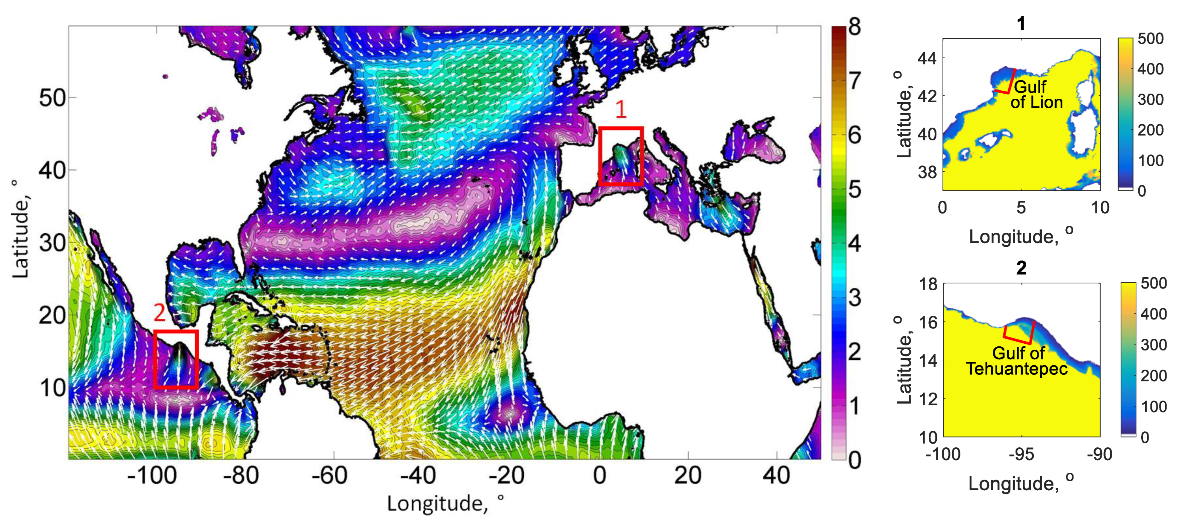
2. Data and Methods
2.1. Data Description
2.2. Method of Wave Measurements
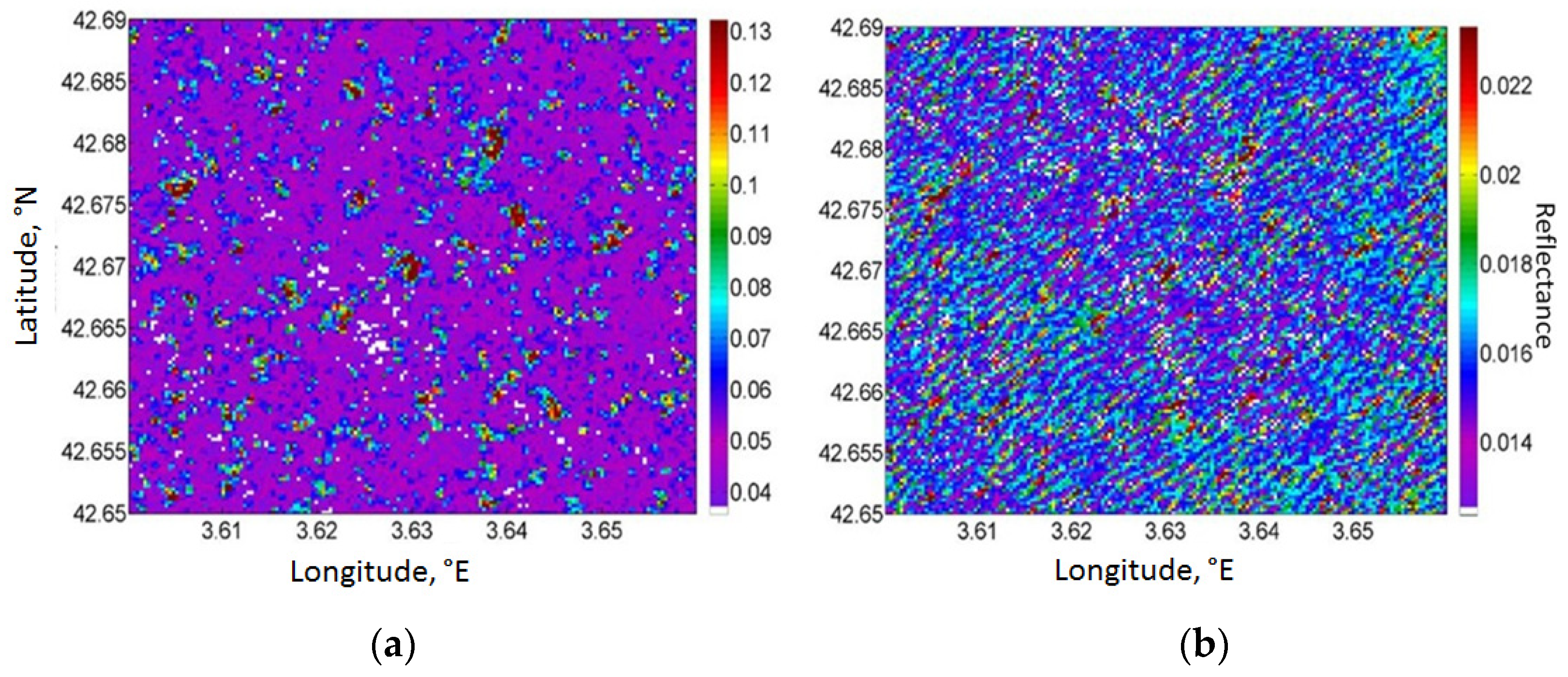
2.3. Method of Wave Breaking Measurements
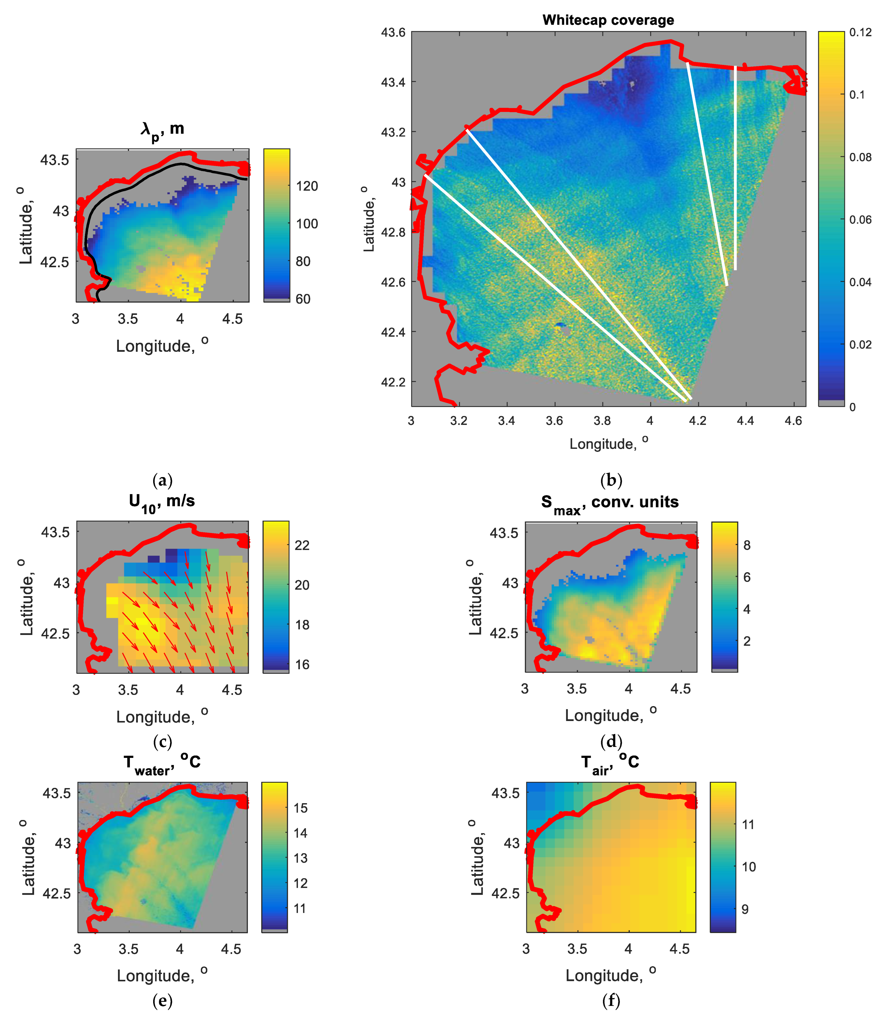
3. Results
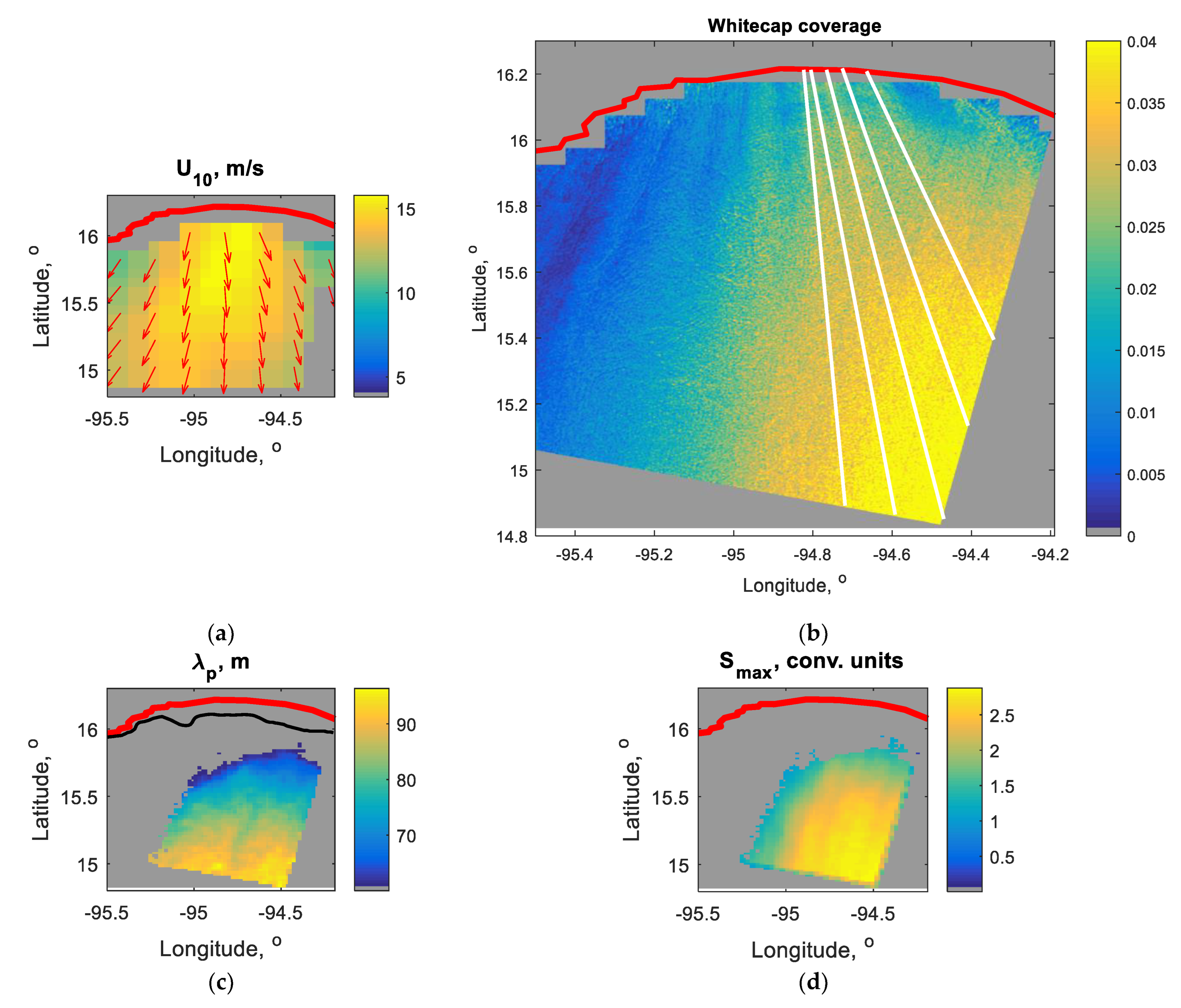
3.1. Approach to Data Analysis
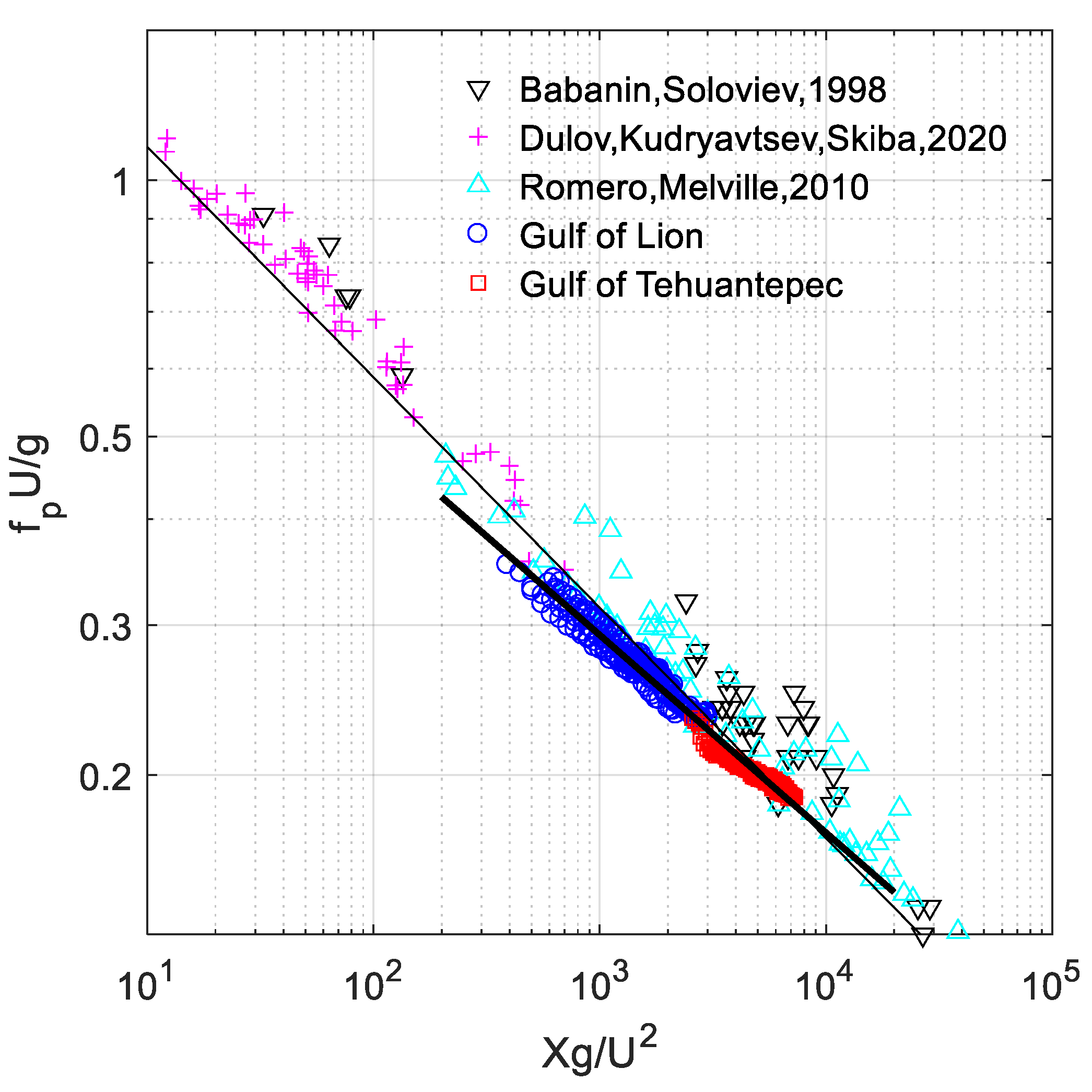
3.2. Spectral Peak Frequency versus Fetch
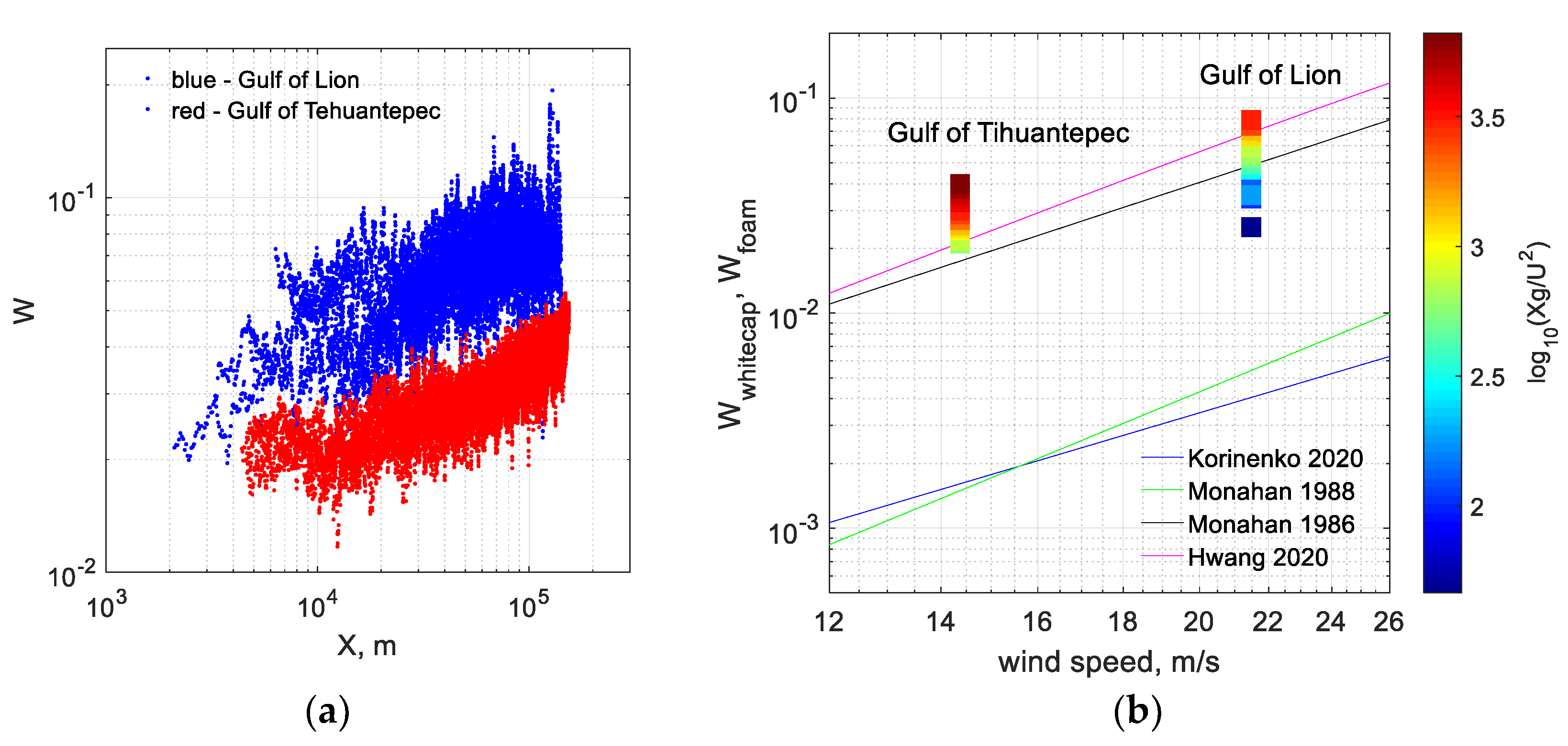
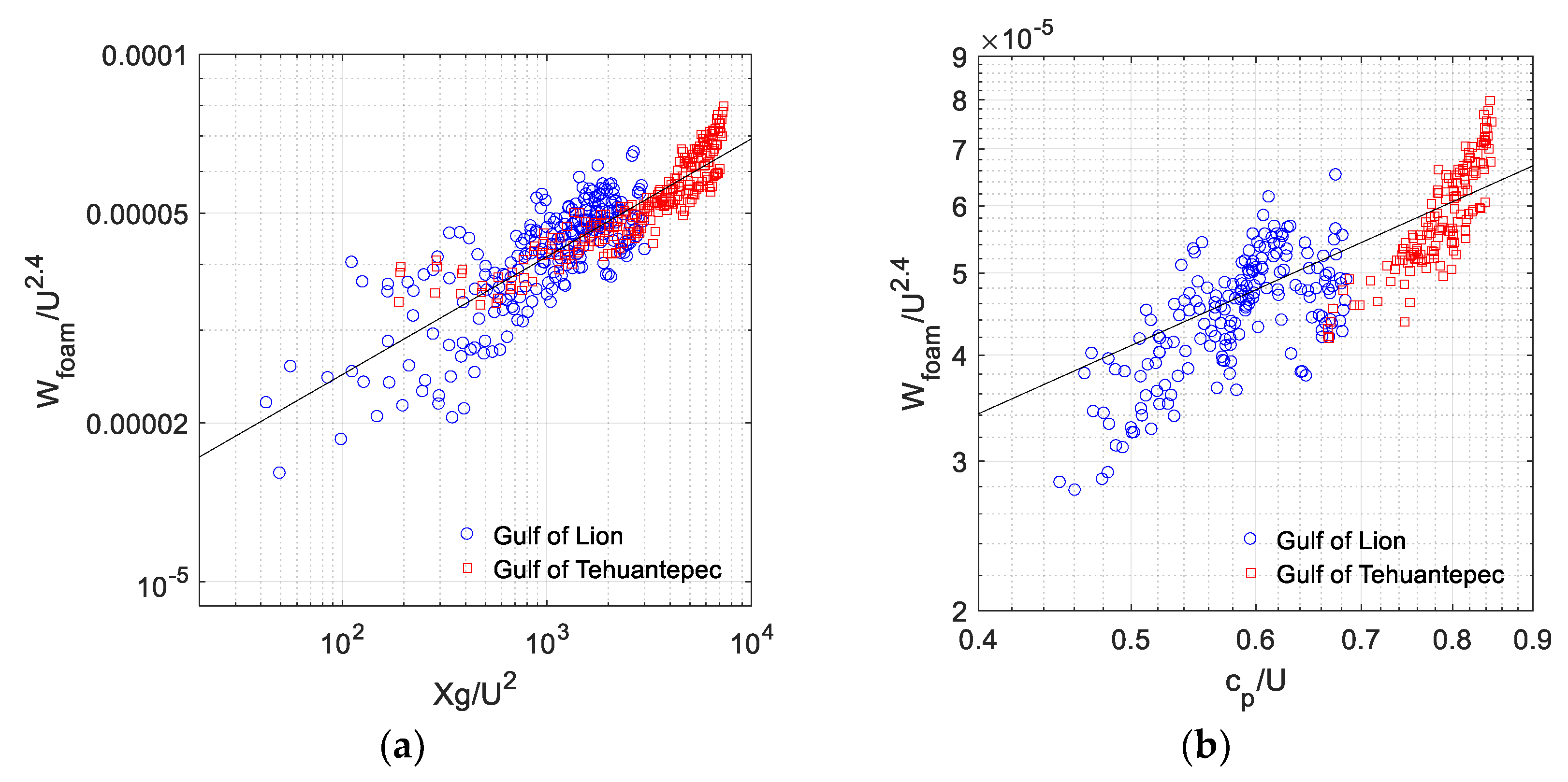
3.3. Whitecap Coverage versus Fetch
4. Discussion
5. Conclusions
Author Contributions
Funding
Data Availability Statement
Acknowledgments
Conflicts of Interest
Appendix A. Meteorological Conditions
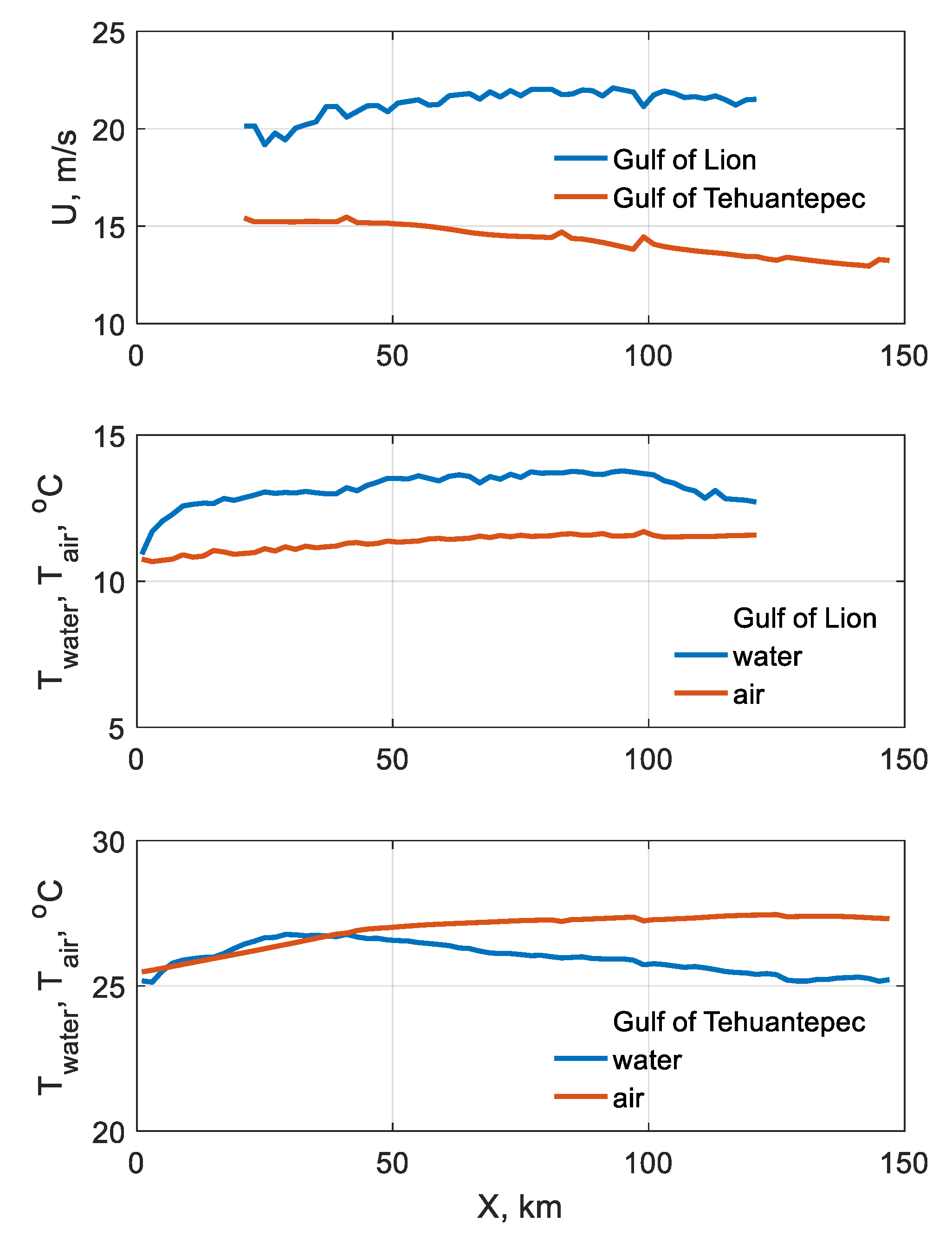

| Gulf of Lion | Gulf of Tehuantepec | |||||
|---|---|---|---|---|---|---|
| min | max | min | max | |||
| , m/s | 19.2 | 22.1 | 0.4 | 13.0 | 15.5 | 0.5 |
| , °C | 10.9 | 13.8 | <0.01 | 25.1 | 27.5 | <0.1 |
| , °C | 10.7 | 11.7 | <0.02 | 25.5 | 27.5 | <0.1 |
| , °C | −2.3 | −0.2 | <0.04 | −0.4 | 2.2 | 0.07 |
References
- Kitaigorodskii, S. Applications of the theory of similarity to the analysis of wind-generated wave motion as a stochastic process. Bull. Acad. Sci. USSR, Geophys. Ser. 1962, 1, 105–117. [Google Scholar]
- Hasselmann, K.; Barnett, T.P.; Bouws, E.; Carlson, H.; Cartwright, D.E.; Enke, K.; Ewing, J.A.; Gienapp, H.; Hasselmann, D.E.; Kruseman, P.; et al. Measurements of Wind-Wave Growth and Swell Decay during the Joint North Sea Wave Project (JONSWAP). Ergnzungsh. zur Dtsch. Hydrogr. Zeitschrift R. 1973, A, 95. [Google Scholar]
- Komen, G.J.; Cavaleri, L.; Donelan, M.A.; Hasselmann, K.; Hasselmann, S.; Janssen, P.A.E.M. Dynamics and Modelling of Ocean Waves; Cambridge University Press: Cambridge, UK, 1994; ISBN 0-521-47047-1. [Google Scholar]
- Ardhuin, F.; Herbers, T.H.C.; Watts, K.P.; van Vledder, G.P.; Jensen, R.; Graber, H.C. Swell and Slanting-Fetch Effects on Wind Wave Growth. J. Phys. Oceanogr. 2007, 37, 908–931. [Google Scholar] [CrossRef]
- Romero, L.; Melville, W.K. Airborne Observations of Fetch-Limited Waves in the Gulf of Tehuantepec. J. Phys. Oceanogr. 2010, 40, 441–465. [Google Scholar] [CrossRef]
- Hwang, P.A.; García-Nava, H.; Ocampo-Torres, F.J. Observations of Wind Wave Development in Mixed Seas and Unsteady Wind Forcing. J. Phys. Oceanogr. 2011, 41, 2343–2362. [Google Scholar] [CrossRef]
- Dulov, V.; Kudryavtsev, V.; Skiba, E. On fetch- and duration-limited wind wave growth: Data and parametric model. Ocean Model. 2020, 153, 101676:1–101676:9. [Google Scholar] [CrossRef]
- Badulin, S.I.; Babanin, A.V.; Zakharov, V.E.; Resio, D. Weakly turbulent laws of wind-wave growth. J. Fluid Mech. 2007, 591, 339–378. [Google Scholar] [CrossRef]
- Zakharov, V.E.; Badulin, S.I.; Hwang, P.A.; Caulliez, G. Universality of sea wave growth and its physical roots. J. Fluid Mech. 2015, 780, 503–535. [Google Scholar] [CrossRef]
- Zakharov, V.E.; Resio, D.; Pushkarev, A. Balanced source terms for wave generation within the Hasselmann equation. Nonlin. Processes Geophys. 2017, 24, 581–597. [Google Scholar] [CrossRef]
- Pushkarev, A.; Zakharov, V. Limited fetch revisited: Comparison of wind input terms, in surface wave modeling. Ocean Model. 2016, 103, 18–37. [Google Scholar] [CrossRef]
- Zakharov, V.E.; Badulin, S.I.; Geogjaev, V.V.; Pushkarev, A.N. Weak-turbulent theory of wind-driven sea. Earth Space Sci. 2019, 6, 540–556. [Google Scholar] [CrossRef]
- Kudryavtsev, V.; Golubkin, P.; Chapron, B. A simplified wave enhancement criterion for moving extreme events. J. Geophys. Res. Oceans 2015, 120, 7538–7558. [Google Scholar] [CrossRef]
- Kudryavtsev, V.; Yurovskaya, M.; Chapron, B. 2D parametric model for surface wave development under varying wind field in space and time. J. Geophys. Res. Oceans 2021, 126, e2020JC016915. [Google Scholar] [CrossRef]
- Kudryavtsev, V.; Yurovskaya, M.; Chapron, B. Self-similarity of surface wave developments under tropical cyclones. J. Geophys. Res. Oceans 2021, 126, e2020JC016916. [Google Scholar] [CrossRef]
- Sharkov, E.A. Breaking Ocean Waves: Geometry, Structure, and Remote Sensing; Springer/Praxis: Berlin/Heidelberg, Germany, 2007; 278p, ISBN 978-3-540-29827-4. [Google Scholar]
- Babanin, A. Breaking of ocean surface waves. Acta Phys. Slov. 2009, 59, 305–535. [Google Scholar] [CrossRef]
- Kleiss, J.M.; Melville, W.K. Observations of wave breaking kinematics in fetch-limited seas. J. Phys. Oceanogr. 2010, 40, 2575–2604. [Google Scholar] [CrossRef]
- Sutherland, P.; Melville, W.K. Field measurements and scaling of ocean surface wave-breaking statistics. J. Geophys. Res. Lett. 2013, 40, 3074–3079. [Google Scholar] [CrossRef]
- Brumer, S.E.; Zappa, C.J.; Brooks, I.M.; Tamura, H.; Brown, S.M.; Blomquist, B.W.; Cifuentes-Lorenzen, A. Whitecap coverage dependence on wind and wave statistics as observed during SO GasEx and HiWinGS. J. Phys. Oceanogr. 2017, 47, 2211–2235. [Google Scholar] [CrossRef]
- Korinenko, A.E.; Malinovsky, V.V.; Kudryavtsev, V.N.; Dulov, V.A. Statistical Characteristics of Wave Breakings and their Relation with the Wind Waves’ Energy Dissipation Based on the Field Measurements. Phys. Oceanogr. 2020, 27, 472–488. [Google Scholar] [CrossRef]
- Dulov, V.A.; Korinenko, A.E.; Kudryavtsev, V.N.; Malinovsky, V.V. Modulation of Wind-Wave Breaking by Long Surface Waves. Remote Sens. 2021, 13, 2825. [Google Scholar] [CrossRef]
- Rapp, R.J.; Melville, W.K. Laboratory measurements of deep-water breaking waves. Philos. Trans. R. Soc. Lond. Ser. A Math. Phys. Sci. 1990, 331, 735–800. [Google Scholar]
- Lamarre, E.; Melville, W.K. Air entrainment and dissipation in breaking waves. Nature 1991, 351, 469–472. [Google Scholar]
- Anguelova, M.D.; Huq, P. Characteristics of bubble clouds at various wind speeds. J. Geophys. Res. 2012, 117, C03036. [Google Scholar] [CrossRef]
- Lim, H.-J.; Chang, K.-A.; Huang, Z.-C.; Na, B. Experimental study on plunging breaking waves in deep water. J. Geophys. Res. Oceans 2015, 120, 2007–2049. [Google Scholar] [CrossRef]
- Yang, X.; Potter, H. A Novel Method to Discriminate Active from Residual Whitecaps Using Particle Image Velocimetry. Remote Sens. 2021, 13, 4051. [Google Scholar] [CrossRef]
- Wang, D.; Josset, D.; Savelyev, I.; Anguelova, M.; Cayula, S.; Abelev, A. An Experimental Study on Measuring Breaking-Wave Bubbles with LiDAR Remote Sensing. Remote Sens. 2022, 14, 1680. [Google Scholar] [CrossRef]
- Iafrati, A. Energy dissipation mechanisms in wave breaking processes: Spilling and highly aerated plunging breaking events. J. Geophys. Res. 2011, 116, C07024. [Google Scholar] [CrossRef]
- Deike, L.; Melville, K.; Popinet, S. Air entrainment and bubble statistics in breaking waves. J. Fluid Mech. 2016, 801, 91–129. [Google Scholar] [CrossRef]
- Druzhinin, O.A. On the Transfer of Microbubbles by Surface Waves. Izv. Atmos. Ocean. Phys. 2022, 58, 507–515. [Google Scholar] [CrossRef]
- Bortkovskii, R.S. Air-Sea Exchange of Heat and Moisture during Storms; Reidel Dordrecht: Dordrecht, The Netherlands; Springer: Berlin/Heidelberg, Germany, 1987; 190p. [Google Scholar]
- Thorpe, S.A. Bubble clouds and the dynamics of the upper ocean. Q. J. R. Mrfeorol. Soc. 1992, 118, 1–22. [Google Scholar] [CrossRef]
- Cavaleri, L.; Fox-Kemper, B.; Hemer, M. Wind Waves in the Coupled Climate System. Bull. Amer. Meteor. Soc. 2012, 93, 1651–1661, Retrieved 28 February 2023. [Google Scholar] [CrossRef]
- Iafrati, A.; Babanin, A.; Onorato, M. Modeling of oceanatmosphere interaction phenomena during the breaking of modulated wave trains. J. Comput. Phys. 2014, 271, 151–171. [Google Scholar] [CrossRef]
- Sutherland, P.; Melville, W.K. Field measurements of surface and near-surface turbulence in the presence of breaking waves. J. Phys. Oceanogr. 2015, 45, 943–965. [Google Scholar] [CrossRef]
- Shin, Y.; Deike, L.; Romero, L. Modulation of bubble-mediated CO2 gas transfer due to wave-current interactions. J. Geophys. Res. Lett. 2022, 49, e2022GL100017. [Google Scholar] [CrossRef]
- de Leeuw, G.; Andreas, E.; Anguelova, M.D.; Fairall, C.; Lewis, C.; O’Dowd, M.; Schulz, M.; Schwartz, S. Production flux of sea spray aerosol. Rev. Geophys. 2011, 49, RG2001. [Google Scholar] [CrossRef]
- Woolf, D.K. Bubbles and the air-sea transfer velocity of gases. Atmos. Ocean 1993, 31, 517–540. [Google Scholar] [CrossRef]
- Wanninkhof, R.; Asher, W.E.; Ho, D.T.; Sweeney, C.; McGillis, W.R. Advances in quantifying air-sea gas exchange and environmental forcing. Annu. Rev. Mar. Sci. 2009, 1, 213–244. [Google Scholar] [CrossRef]
- Fairall, C.; Keppert, J.; Holland, G. The effect of sea spray on surface energy transport over the ocean. Global Atmos. Ocean Syst. 1994, 2, 121–142. [Google Scholar]
- Andreas, E.L.; Persson, P.P.G.; Hare, J.E. A bulk turbulent air-sea flux algorithm for high-wind, spray conditions. J. Phys. Oceanogr. 2008, 38, 1581–1596. [Google Scholar] [CrossRef]
- Xu, X.; Voermans, J.J.; Moon, I.-J.; Liu, Q.; Guan, C.; Babanin, A.V. Sea spray impacts on Tropical Cyclone Olwyn using a coupled atmosphere-ocean-wave model. J. Geophys. Res. Oceans 2022, 127, e2022JC018557. [Google Scholar] [CrossRef]
- Reul, N.; Chapron, B.; Zabolotskikh, E.; Donlon, C.; Quilfen, Y.; Guimbard, S.; Piolle, J.F. A revised L-band radio-brightness sensitivity to extreme winds under Tropical Cyclones: The five year SMOS-storm database. Remote Sens. Environ. 2016, 180, 274–291. [Google Scholar] [CrossRef]
- Hwang, P.A. High-wind drag coefficient and whitecap coverage derived from microwave radiometer observations in tropical cyclones. J. Phys. Oceanogr. 2018, 48, 2221–2232. [Google Scholar] [CrossRef]
- Sharkov, E.A. Passive microwave Remote Sensing of the Earth: Physical Foundations; Springer/Praxis: Berlin/Heidelberg, Germany; New York, NY, USA; Paris, France; Tokyo, Japan, 2003; 613p, ISBN 3-540-43946-3. [Google Scholar]
- Reul, N.; Chapron, B. A model of sea-foam thickness distribution for passive microwave remote sensing applications. J. Geophys. Res. 2003, 108, C103321. [Google Scholar] [CrossRef]
- Anguelova, M.D.; Webster, F. Whitecap coverage from satellite measurements: A first step toward modeling the variability of oceanic whitecaps. J. Geophys. Res. 2006, 111, C03017:1–C03017:23. [Google Scholar] [CrossRef]
- Anguelova, M.D.; Gaiser, P.M. Microwave emissivity of sea foam layers with vertically inhomogeneous dielectric properties. Remote Sens. Environ. 2013, 139, 81–96. [Google Scholar] [CrossRef]
- Hwang, P.A. Whitecap Observations by Microwave Radiometers: With Discussion on Surface Roughness and Foam Contributions. Remote Sens. 2020, 12, 2277. [Google Scholar] [CrossRef]
- Kahma, K.K.; Calkoen, C.J. Reconciling Discrepancies in the Observed Growth of Wind-generated Waves. J. Phys. Oceanogr. 1992, 22, 1389–1405. [Google Scholar] [CrossRef]
- Babanin, A.V.; Soloviev, Y.P. Field Investigation of Transformation of the Wind Wave Frequency Spectrum with Fetch and the Stage of Development. J. Phys. Oceanogr. 1998, 28, 563–576. [Google Scholar] [CrossRef]
- Dobson, F.; Perrie, W.; Toulany, B. On the deep-water fetch laws for wind-generated surface gravity waves. Atmosphere-Ocean 1989, 27, 210–236. [Google Scholar] [CrossRef]
- Kraan, C.; Oost, W.A.; Janssen, P.A.E.M. Wave energy dissipation by whitecaps. J. Atmos. Oceanic Technol. 1996, 13, 262–267. [Google Scholar] [CrossRef]
- Lafon, C.; Piazzola, J.; Forget, P.; Le Calve, O.; Despiau, S. Analysis of the variations of the whitecap fraction as measured in a coastal zone. Boundary Layer Meteorol. 2004, 111, 339–360. [Google Scholar] [CrossRef]
- Guan, C.; Hu, W.; Sun, J.; Li, R. The whitecap coverage model from breaking dissipation parameterizations of wind waves. J. Geophys. Res. 2007, 112, C05031. [Google Scholar] [CrossRef]
- Callaghan, A.H.; Deane, G.B.; Stokes, M.D. Observed physical and environmental causes of scatter in whitecap coverage values in a fetch-limited coastal zone. J. Geophys. Res. 2008, 113, C05022. [Google Scholar] [CrossRef]
- Bortkovskii, R.S.; Novak, V.A. Statistical dependencies of sea state on water temperature and wind-wave age. J. Mar. Syst. 1993, 4, 161–169. [Google Scholar] [CrossRef]
- Stramska, M.; Petelski, T. Observations of oceanic whitecaps in the north polar waters of the Atlantic. J. Geophys. Res. 2003, 108, 3086. [Google Scholar] [CrossRef]
- Goddijn-Murphy, L.; Woolf, D.; Callaghan, A. Parameterizations and Algorithms for Oceanic Whitecap Coverage. J. Phys. Oceanogr. 2011, 41, 742–756. [Google Scholar] [CrossRef]
- Sugihara, Y.; Tsumori, H.; Ohga, T.; Yoshioka, H.; Serizawa, S. Variation of whitecap coverage with wave-field conditions. J. Mar. Syst. 2007, 66, 47–60. [Google Scholar] [CrossRef]
- Salisbury, D.J.; Anguelova, M.D.; Brooks, I.M. On the variability of whitecap fraction using satellite-based observations. J. Geophys. Res. Oceans. 2013, 118, 6201–6222. [Google Scholar]
- Lafon, C.; Piazzola, J.; Forget, P.; Despiau, S. Whitecap coverage in coastal environment for steady and unsteady wave field conditions. J. Mar. Syst. 2007, 66, 38–46. [Google Scholar] [CrossRef]
- Kubryakov, A.A.; Kudryavtsev, V.N.; Stanichny, S.V. Application of Landsat imagery for the investigation of wave breaking. Remote Sens. Environ. 2021, 253, 112144:1–112144:18. [Google Scholar] [CrossRef]
- Kudryavtsev, V.; Yurovskaya, M.; Chapron, B.; Collard, F.; Donlon, C. Sun glitter Imagery of Ocean Surface Waves. Part 1: Directional spectrum retrieval and validation. J. Geophys. Res. Oceans. 2017, 122, 1369–1383. [Google Scholar] [CrossRef]
- Kudryavtsev, V.; Yurovskaya, M.; Chapron, B.; Collard, F.; Donlon, C. Sun glitter Imagery of Ocean Surface Waves. Part 2: Waves transformation on the Ocean Currents. J. Geophys. Res. Oceans 2017, 122, 1384–1399. [Google Scholar] [CrossRef]
- Ardhuin, F.; Alday, M.; Yurovskaya, M. Total surface current vector and shear from a sequence of satellite images: Effect of waves in opposite directions. J. Geophys. Res. Oceans 2021, 126, e2021JC017342. [Google Scholar] [CrossRef]
- Bondur, V.; Dulov, V.; Kozub, V.; Murynin, A.; Yurovskaya, M.; Yurovsky, Y. Validation of the Satellite Method for Measuring Spectra of Spatially Inhomogeneous Sea Waves. J. Mar. Sci. Eng. 2022, 10, 1510. [Google Scholar] [CrossRef]
- Zhang, H.; Lou, X.; Li, Y.; Shi, A.; Li, D.; Fu, B. Whitecap features induced by submarine sand waves in stereo optical imagery. J. Geophys. Res. Oceans 2015, 120, 6225–6233. [Google Scholar] [CrossRef]
- Anguelova, M.D.; Bettenhausen, M.H. Whitecap Fraction from Satellite Measurements: Algorithm Description. J. Geophys. Res. Oceans 2019, 124, 1827–1857. [Google Scholar] [CrossRef]
- Queffeulou, P.; Bentamy, A. Analysis of Wave Height Variability Using Altimeter Measurements: Application to the Mediterranean Sea. J. Atmos. Oceanic Technol. 2007, 24, 2078–2092. [Google Scholar] [CrossRef]
- Barbariol, F.; Davison, S.; Falcieri, F.M.; Ferretti, R.; Ricchi, A.; Sclavo, M.; Benetazzo, A. Wind Waves in the Mediterranean Sea: An ERA5 Reanalysis Wind-Based Climatology. Front. Mar. Sci 2021, 8, 760614. [Google Scholar] [CrossRef]
- Renault, L.; Chiggiato, J.; Warner, J.C.; Gomez, M.; Vizoso, G.; Tintoré, J. Coupled atmosphere-ocean-wave simulations of a storm event over the Gulf of Lion and Balearic Sea. J. Geophys. Res. 2012, 117, C09019. [Google Scholar] [CrossRef]
- Romero, L.; Melville, W.K. Numerical Modeling of Fetch-Limited Waves in the Gulf of Tehuantepec. J. Phys. Oceanogr. 2010, 40, 466–486. [Google Scholar] [CrossRef]
- Bentamy, A.; Croize-Fillon, D.; Perigaud, C. Characterization of ASCAT measurements based on buoy and QuikSCAT wind vector observations. Ocean Science 2008, 4, 265–274. [Google Scholar] [CrossRef]
- Aleskerova, A.A.; Kubryakov, A.A.; Stanichny, S.V. A two channel method for retrieval of the Black Sea surface temperature from Landsat-8 measurements. Izv. Atmos. Ocean Phys. 2016, 52, 1155–1161. [Google Scholar] [CrossRef]
- Schott, J.R.; Gerace, A.; Woodcock, C.E.; Wang, S.; Zhu, Z.; Wynne, R.H.; Blinn, C.E. The impact of improved signal-to-noise ratios on algorithm performance: Case studies for Landsat class instruments. Remote Sens. Environ. 2016, 185, 37–45. [Google Scholar] [CrossRef]
- Yurovskaya, M.V.; Dulov, V.A.; Chapron, B.; Kudryavtsev, V.N. Directional short wind wave spectra derived from the sea surface photography. J. Geophys. Res. 2013, 118, 4380–4394. [Google Scholar] [CrossRef]
- Bendat, J.; Piersol, A. Random Data: Analysis and Measurement Procedures, Fourth edition; John Wiley & Sons, Inc.: Hoboken, NJ, USA, 2010; 600p. [Google Scholar] [CrossRef]
- Koepke, P. Effective reflectance of oceanic whitecaps. Appl. Opt. 1984, 23, 1816–1824. [Google Scholar] [CrossRef] [PubMed]
- Mironov, A.S.; Dulov, V.A. Detection of wave breaking using sea surface video records. Meas. Sci. Technol. 2008, 19, 015405. [Google Scholar] [CrossRef]
- Monahan, E.C.; Woolf, D.K. Comments on “Variations of whitecap coverage with wind stress and water temperature”. J. Phys. Oceanogr. 1989, 19, 706–709. [Google Scholar] [CrossRef]
- Monahan, E.C.; Lu, M. Acoustically relevant bubble assemblages and their dependence on meteorological parameters. IEEE J. Oceanic Eng. 1990, 15, 340–349. [Google Scholar] [CrossRef]
- Monahan, E.C.; Wilson, M.B.; Woolf, D.K. HEXMAX whitecap climatology. In Humidity Exchange Over the Sea Min Experiment (HEXMAX), Analysis and Interpretation, Proceedings of the NATO Advanced Workshop, Epe, The Netherlands, 25–29 April 1988; Oost, W.A., Smith, S.D., Katsaros, K.B., Eds.; University of Washington: Seattle, WA, USA, 1988; pp. 105–115. [Google Scholar]
- Monahan, E.C.; O’Muircheartaigh, I. Whitecaps and the passive remote sensing of the ocean surface. Int. J. Remote Sens. 1986, 7, 627–642. [Google Scholar] [CrossRef]
- Wu, J. Variations of whitecap coverage with wind stress and water temperature. J. Phys. Oceanogr. 1988, 18, 1448–1453. [Google Scholar] [CrossRef]
- Hwang, P.A.; Sletten, M.A. Energy dissipation of wind-generated waves and whitecap coverage. J. Geophys. Res. 2008, 113, C02012:1–C02012:12. [Google Scholar] [CrossRef]
- Anguelova, M.; Hwang, P. Using Energy Dissipation Rate to Obtain Active Whitecap Fraction. J. Phys. Oceanogr. 2016, 46, 461–481. [Google Scholar] [CrossRef]
- Callaghan, A. On the Relationship between the Energy Dissipation Rate of Surface-Breaking Waves and Oceanic Whitecap Coverage. J. Phys. Oceanogr. 2018, 48, 2609–2626. [Google Scholar] [CrossRef]
- Phillips, O.M. Spectral and statistical properties of the equilibrium range in wind-generated gravity waves. J. Fluid Mech. 1985, 156, 505–531. [Google Scholar] [CrossRef]
- Hanson, J.L.; Phillips, O.M. Wind sea growth and dissipation in the open ocean. J. Phys. Oceanogr. 1999, 29, 1633–1648. [Google Scholar] [CrossRef]
- Zakharov, V.E.; Resio, D.; Pushkarev, A. New wind input term consistent with experimental, theoretical and numerical considerations. arXiv 2012, arXiv:1212.1069. [Google Scholar] [CrossRef]
- Reul, N.; Chapron, B.; Zabolotskikh, E.; Donlon, C.; Mouche, A.; Tenerelli, J.; Collard, F.; Piolle, J.-F.; Fore, A.; Yueh, S.; et al. A New Generation of Tropical Cyclone Size Measurements from Space. Bull. Am. Meteor. Soc. 2017, 98, 2367–2385. [Google Scholar] [CrossRef]


Disclaimer/Publisher’s Note: The statements, opinions and data contained in all publications are solely those of the individual author(s) and contributor(s) and not of MDPI and/or the editor(s). MDPI and/or the editor(s) disclaim responsibility for any injury to people or property resulting from any ideas, methods, instructions or products referred to in the content. |
© 2023 by the authors. Licensee MDPI, Basel, Switzerland. This article is an open access article distributed under the terms and conditions of the Creative Commons Attribution (CC BY) license (https://creativecommons.org/licenses/by/4.0/).
Share and Cite
Dulov, V.A.; Skiba, E.V.; Kubryakov, A.A. Landsat-8 Observations of Foam Coverage under Fetch-Limited Wave Development. Remote Sens. 2023, 15, 2222. https://doi.org/10.3390/rs15092222
Dulov VA, Skiba EV, Kubryakov AA. Landsat-8 Observations of Foam Coverage under Fetch-Limited Wave Development. Remote Sensing. 2023; 15(9):2222. https://doi.org/10.3390/rs15092222
Chicago/Turabian StyleDulov, Vladimir A., Ekaterina V. Skiba, and Arseny A. Kubryakov. 2023. "Landsat-8 Observations of Foam Coverage under Fetch-Limited Wave Development" Remote Sensing 15, no. 9: 2222. https://doi.org/10.3390/rs15092222