UAV Network Path Planning and Optimization Using a Vehicle Routing Model

Abstract

Unmanned aerial vehicle (UAV) remote sensing has been applied in various fields due to its rapid implementation ability and high-resolution imagery. Single-UAV remote sensing has low efficiency and struggles to meet the growing demands of complex aerial remote sensing tasks, posing challenges for practical applications. Using multiple UAVs or a UAV network for remote sensing applications can overcome the difficulties and provide large-scale ultra-high-resolution data rapidly. UAV network path planning is required for these important applications. However, few studies have investigated UAV network path planning for remote sensing observations, and existing methods have various problems in practical applications. This paper proposes an optimization algorithm for UAV network path planning based on the vehicle routing problem (VRP). The algorithm transforms the task assignment problem of the UAV network into a VRP and optimizes the task assignment result by minimizing the observation time of the UAV network. The optimized path plan prevents route crossings effectively. The accuracy and validity of the proposed algorithms were verified by simulations. Moreover, comparative experiments with different task allocation objectives further validated the applicability of the proposed algorithm for various remote sensing applications

1. Introduction

Unmanned aerial vehicle (UAV) remote sensing has the advantages of high-frequency coverage, high-resolution imagery, and flexible operations. It has been widely applied in emergency rescue [1], natural disaster assessment [2], environmental monitoring [3], the mobile communications community [4] and other areas in recent years [5,6,7,8,9,10,11,12,13,14,15]. UAV path planning is an essential task in remote sensing projects and affects the quality and efficiency of remote sensing data acquisition. Therefore, it is necessary to research UAV path planning algorithms. Most studies on this topic have focused on small-scale operation by a single UAV and used sequential and interval flight path methods [16]. Research on path planning for complex polygonal task areas [17,18] and in complex terrains [19] has improved the performance of single-UAV remote sensing operations. However, due to increasingly complex aerial remote sensing tasks, single-UAV operations cannot meet the efficiency and response speed requirements, limiting the use of UAV remote sensing for multiple applications. Using multiple UAVs or a UAV network enables the acquisition of large amounts of ultra-high-resolution data rapidly, and the synergistic observation of multi-load networks provides a rich data source for various remote sensing applications [20]. Unlike single-UAV flight path planning, network path planning requires the allocation of multiple UAVs according to the optimal path planning strategy to complete remote sensing tasks. The optimization goal of task assignment is to obtain the shortest observation time or the least number of UAVs.

Task assignment is a crucial component of the UAV network path planning algorithm; thus, current research has focused on improving it. Extensive studies have been conducted domestically and internationally on multi-UAV cooperative operation path planning algorithms, but relatively few studies have investigated UAV network path planning. However, task allocation remains a key step in solving both problems. Peng et al. [21] analyzed multi-UAV path planning for multi-UAV cooperative operations and divided sub-regions based on UAV performance indices. They performed task assignment by segmenting the regions based on their areas. However, this approach only considered the sub-region size and not its characteristics. In contrast, Chen et al. [22] proposed a task allocation method that incorporated UAV performance indices and the geometric features of sub-regions. Agarwal et al. [23] divided the observation area into multiple parallel polygons for task allocation based on UAV performance indices. Several studies have employed decomposition algorithms to partition the area and allocate tasks [24,25]. These studies employed region segmentation algorithms to partition the area and assign tasks. However, UAV obstacle avoidance in the sub-regions was not considered, which could increase risks during operations. Several researchers have employed greedy algorithms to assign task regions based on the probability of a moving target appearing in a certain region [26]. This type of algorithm has been widely utilized for military applications, and several task assignment algorithms have been applied in military target tracking [27]. These methods allocate tasks to sub-regions based on UAV performance or using region segmentation algorithms, and then plan paths within each sub-region. However, these methods are prone to the risk of UAV collisions between sub-regions and are difficult to apply in practice.

Numerical optimization methods can directly allocate tasks without dividing sub-regions, i.e., transforming the UAV network path planning problem into a vehicle routing problem (VRP). The VRP is an optimization problem that aims to find the optimal routes of multiple vehicles serving multiple customers repeatedly in different geographical locations using a given road network. The task assignment problem in UAV network path planning is transformed into the VRP by treating the start and end shooting points of each planned route as customers. Gustavo et al. [28] proposed a solution that planned the path of a single UAV to cover the area and then calculate the number of UAVs that could cover the area in the shortest time to assign tasks to the UAVs. However, the algorithm does not consider obstacle avoidance among UAVs, which requires optimization. In addition, researchers proposed assigning tasks by minimizing the number of UAVs in the network [29], but the algorithm did not consider the observation time constraint. Once faced with sudden and acute remote sensing tasks, the observation time had to be decreased by increasing the number of UAVs.

The task allocation outcome significantly impacts the effectiveness of the UAV network operation. Thus, a reasonable task assignment solution is essential to ensure the efficient completion of UAV remote sensing tasks. This paper proposes an optimization algorithm for UAV network path planning based on the VRP model, which considers obstacle avoidance among UAVs during task allocation.

2. Methods

2.1. Problem Definition

Task assignment is a combinatorial optimization and integer planning problem in operations research. The VRP originally refers to the problem where a set of vehicles must only visit a set of customers once located in different geographical locations to find an optimal set of execution routes in a given traffic road network [30]. The vehicle routing model can be employed to solve the UAV network path planning problem by transforming the task assignment problem into a numerical optimization problem using mathematical planning methods. More specifically, the task allocation problem is transformed into the VRP by treating the start and end shooting points of each planned route as customers. The problem is then solved by finding the optimal allocation using a specific objective function. Additionally, considering UAV performance in task allocation is a critical re AV. search direction in this study. The proposed algorithm allocates tasks to UAVs after conducting single-UAV flight path planning, and the optimization goal is to minimize the observation time when calculating the number of UAVs in the network. Route crossing is prevented by adding an obstacle avoidance constraint. The technical route of the optimization algorithm is shown in Figure 1.

The proposed optimization algorithm allocates tasks to the available UAVs in an optimal manner, such that the total observation time is minimized and the UAVs do not collide with each other during their flights. The task allocation process also considers the constraints, such as the number of available UAVs, the number of customers to be visited, and the fact that each customer can only be visited once. By solving the VRP problem with these constraints and objectives, the algorithm can obtain the final results of the UAV network path planning model, which can be used to perform remote sensing tasks efficiently.

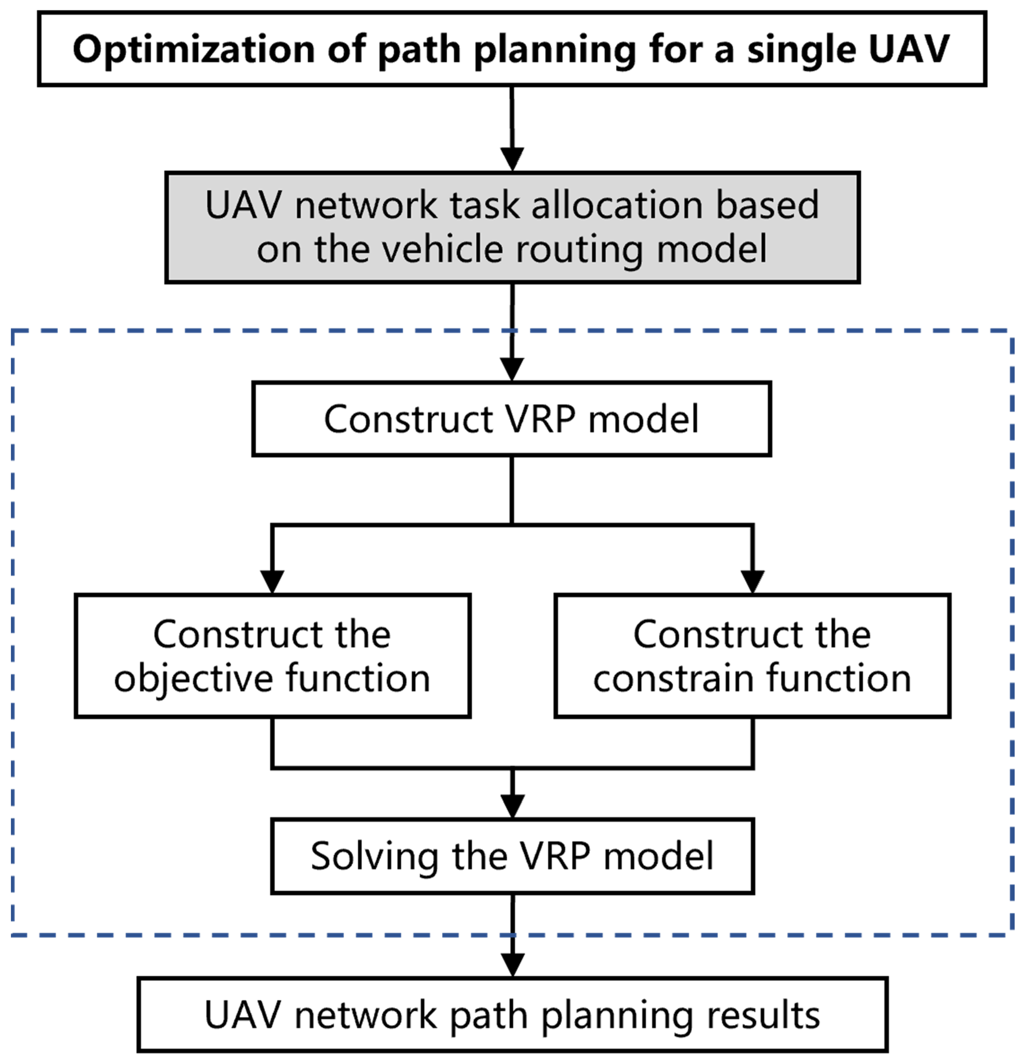
2.2. Model Establishment

The basic VRP model is established as follows. A graph, G = (V, E), is constructed to transform the task assignment problem of the UAV network into a VRP. The node set V consists of the endpoints of each route and the UAV launch position. Each node in the graph is numbered sequentially; the field station is node 1, the starting point of the first route is node 2, and the endpoint of the first route is 3. Similarly, the starting point and endpoint of subsequent routes are numbered sequentially. The edge set E comprises all lines connecting the N nodes of the graph. All nodes are connected by edges to form the graph $G=\left(V,E\right)$, as shown in Figure 2.

The distance between the nodes of graph G is calculated to construct the cost matrix (C), whose elements ($C_{ij}$) represent the Euclidean distance between each node of graph G. For any edge in the set E, there exists $C_{ij}=C_{ji}$, $C_{ij}+C_{jk}\ge C_{ik}$. The matrix (C) has the following form:

$$C=\left[\begin{array}{ccc}\begin{array}{cc}{C}_{11}& C_{12}\\ C_{21}& C_{22}\end{array}& \begin{array}{c}\dots \\ \dots \end{array}& \begin{array}{c}{C}_{1N}\\ C_{2N}\end{array}\\ \begin{array}{cc}⋮& ⋮\end{array}& ⋮& ⋮\\ \begin{array}{cc}{C}_{N1}& C_{N2}\end{array}& \cdots & C_{NN}\end{array}\right]$$

(1)

By constructing graph G, UAV network task allocation is transformed into a VRP. The optimal UAV network task assignment and the task routes of each UAV can be obtained by solving the VRP. Each node except the field station must be visited only once, and the UAVs are constrained by their endurance range and safety issues, which should be considered in the task assignment. The overall task assignment objective is cost minimization.

Before constructing the objective and constraint functions, we define the required constants and variables. The constant $C_{ij}$ represents the cost of traversing the edge $E\left(i,j\right)$, i.e., the flight distance of the UAV from node i to j. The decision variable $X_{ij}^k\in \left\{0,1\right\}$ is used to indicate whether the k-th UAV has flown from node i to j, and the velocity is represented by the constant $V_{ij}^k\in R$. $t_s$ denotes the preparation time before each UAV takes off and the constant T denotes the flight duration of the UAV. The number of UAVs that assigned to this task and the number of UAVs can be launched normally from the field station are denoted as $m\in N$ and $M\in N$, respectively; $N\in N$ is the number of nodes of the graph G, i.e., the number of field stations and the sum of the starting and endpoints of all routes.

The goal of this task allocation method is to minimize the number of dispatched UAVs while ensuring the shortest possible observation time. Based on the above variables, the duration time ($d_k$) between the takeoffs of the first UAV and the k-th UAV can be expressed by Equation (2), and the elapsed flight time of UAV k is given by Equation (3):

$$d_k=t_s\ast \left(k-1\right) \cdot {\displaystyle \sum }_{j=1}^N{X}_{1j}^k , k=1,2,3,\dots ,M$$

(2)

$$T_k={\displaystyle \sum }_{i=1}^N{\displaystyle \sum }_{j=1}^N\frac{C_{ij}·X_{ij}^k}{V_{ij}}+d_k$$

(3)

The observation time of the k-th UAV is defined as the sum of its flight operation time and the waiting time before takeoff, while the observation time of the UAV network is defined as the maximum observation time among all UAVs’ observation times. To minimize the number of launched UAVs and the network observation time, we need to minimize the longest observation time of all UAVs. Therefore, the optimization problem can be represented by the objective function z:

$$z=min max T_k, k=1,2,3\dots ,M$$

(4)

The constraint function of the VRP model includes the following constraints: UAV endurance, the node access rules in the graph, and that there are no route crossings. UAV endurance is the most important constraint. The duration constraint requires that the observation time of each UAV must be less than its endurance to ensure operational safety. Thus, the operating time of UAV k must satisfy the constraint expressed in Equation (5).

$${\displaystyle \sum }_{i=1}^N{\displaystyle \sum }_{j=1}^N\frac{C_{ij}·X_{ij}^k}{V_{ij}}\le T, k=1,2,3\dots ,M$$

(5)

Each route should be traversed only by one UAV except for the field station; therefore, the constraints described in Equations (6) and (7) must be satisfied. Equation (6) ensures that each route is traversed by only one UAV, and Equation (7) ensures that the number of UAVs arriving at a node is the same as the number of UAVs leaving that node.

$${\displaystyle \sum }_{k=1}^M{\displaystyle \sum }_{i=1}^N{X}_{ij}^k=1, j=2,3,4\dots ,M$$

(6)

$${\displaystyle \sum }_{i=1}^N{X}_{ip}^k-{\displaystyle \sum }_{j=1}^N{X}_{pj}^k=0,p=1,2,3\dots ,N,k=1,2,3\dots ,M$$

(7)

UAVs at field stations can have two states: being dispatched on missions or being on standby. Each UAV must satisfy the constraints in Equations (8) and (9). Equation (8) ensures that each UAV is either on standby or takes off only once, while Equation (9) guarantees that each UAV is either dispatched on a mission or lands only once, i.e., each UAV must have either no takeoff or one takeoff and one landing.

$${\displaystyle \sum }_{j=2}^N{X}_{1j}^k\le 1,k=1,2,3\dots ,M$$

(8)

$${\displaystyle \sum }_{j=2}^N{X}_{j1}^k\le 1,k=1,2,3\dots ,M$$

(9)

The standard sub-path elimination constraint [31] is used to ensure that each UAV flies to the operation area for the mission and returns to the field station after the operation, i.e., the route of each UAV starts at the station and ends at the station without internal loops:

$$u_i-u_j+N·{\displaystyle \sum }_{k=1}^M{X}_{ij}^k\le N-1,i,j=2,3,4\dots ,N$$

(10)

where $u_i\in Z,i=2,3,4\dots ,N$.

Unlike the vehicles in VRPs, UAVs must operate on specific routes, and each route can only be visited once by a UAV. In other words, a UAV entering one end of a route must fly out from the other end of that route, turn around, and traverse the next route or return to the station.

This constraint can be reflected in graph G in a way in which a UAV visiting an even-numbered node must visit the next odd-numbered node adjacent to it, and accordingly, a UAV visiting each odd-numbered node must visit the last even-numbered node adjacent to it. Therefore, the constraint of Equation (11) must be satisfied.

$${\displaystyle \sum }_{k=1}^M{X}_{i,i+1}^k+{\displaystyle \sum }_{k=1}^M{X}_{i+1,i}^k=1,i=2,4,6\dots ,N$$

(11)

Furthermore, the constraints expressed in Equations (12) and (13) must be satisfied to prevent UAVs from conducting invalid operations and ensure the safety of UAV network observation. An invalid operation refers to the UAV’s flight across the designated route in its own mission area, which increases the UAV’s operating time and the number of invalid images. Therefore, the avoidance of route crossings should be considered in the task allocation process of UAV network observation. When the algorithm assigns tasks, the UAVs cannot fly across the area, and the flight routes must be adjacent to each other. Equation (12) is the constraint for the even number of routes, while Equation (13) is the constraint for the odd number of routes. The performance of the proposed VRP model is higher than that of the model proposed by Gustavo et al. (hereafter called the original method) because route crossing is prevented.

$${\displaystyle \sum }_{k=1}^M{X}_{i,i+1}^k=\left\{\begin{array}{c}{\displaystyle \sum _{k=1}^M}{X}_{i+1,i+3}^k+{\displaystyle \sum _{k=1}^M}{X}_{i+1,i-1}^k,i=2\\ {\displaystyle \sum _{k=1}^M}{X}_{i+1,i+3}^k+{\displaystyle \sum _{k=1}^M}{X}_{i+1,i-1}^k+{\displaystyle \sum _{k=1}^M}{X}_{i+1,1}^k,i=\left\{2,4,6\dots ,N\right\}\backslash \left\{2,N-1\right\}\\ {\displaystyle \sum _{k=1}^M}{X}_{i+1,1}^k+{\displaystyle \sum _{k=1}^M}{X}_{i+1,i-1}^k,i=N-1\end{array}\right.$$

(12)

$${\displaystyle \sum }_{k=1}^M{X}_{i,i-1}^k=\left\{\begin{array}{c}{\displaystyle \sum _{k=1}^M}{X}_{i-1,1}^k+{\displaystyle \sum _{k=1}^M}{X}_{i-1,i+1}^k,i=3\\ {\displaystyle \sum _{k=1}^M}{X}_{i-1,i+1}^k+{\displaystyle \sum _{k=1}^M}{X}_{i-1,i-3}^k+{\displaystyle \sum _{k=1}^M}{X}_{i-1,1}^k,i=\left\{3,5,7\dots ,N\right\}\backslash \left\{3,N\right\}\\ {\displaystyle \sum _{k=1}^M}{X}_{i-1,1}^k+{\displaystyle \sum _{k=1}^M}{X}_{i-1,i-3}^k,i=N\end{array}\right.$$

(13)

The following equations must also be satisfied to ensure that the number of dispatched UAVs in the task is less than the total number of UAVs available at the field station:

$$m={\displaystyle \sum }_{k=1}^M{\displaystyle \sum }_{j=1}^N{X}_{1,j}^k$$

(14)

$$m\le M$$

(15)

3. Simulations

Simulation experiments were conducted to verify the algorithm’s performance. Since the VRP is a classical mixed-integer linear programming (MILP) problem, the solutions are relatively mature. The task assignment can be obtained by solving the VRP model constructed in the previous section. To solve the VRP, we used the MATLAB toolbox YALMIP, a powerful optimization toolbox that contains more than 20 solvers [32]. CPLEX and Gurobi are widely used solvers for MILP problems. CPLEX is the most used integer solver, and Gurobi can solve large linear projects. They use parallel algorithms to increase the solution speed and have been commonly used to solve VRPs. We employed CPLEX and Gurob in the simulation to solve the VRP and analyze the solution results.

3.1. Observation Area

A complex convex polygon of S (as shown in Figure 3) was used as the observation region in the simulation. Each vertex of the polygon in the observation region S was recorded clockwise $\left\{v_1,v_2,v_3,v_4,v_5\right\}$, and the coordinates of each vertex were labeled as:

$$S=\left\{(14.5,2), (5.6,17), (21,29), (30,20), \left(21.5,3\right)\right\}\times {10}^2$$

(16)

In single-UAV path planning, the initial step is to determine the flight direction of the UAV. Subsequently, the trajectory points and routes can be obtained. Additionally, the optimal starting point for the mission is selected. To determine the flight direction, the minimum span tree algorithm [33] is used to calculate the minimum span of the observation region polygon. The algorithm helps identify the optimal flight direction with the least number of turns for the UAV. Specifically, the vertices and edges corresponding to the minimum span of the observation region S are $v_1$ and edge $v_4{v}_5$, which determine the flight direction of the UAV. The optimal mission starting point is determined based on the relationships between the UAV field station and the observation area to ensure the shortest range of the UAV to and from the station.

3.2. Simulation Results

To evaluate the proposed algorithm’s performance, the simulation experiment used several UAV performance parameters, including the preparation time $t_s$, flight speed and endurance. These assumed values can be adjusted according to different scenarios and UAV models. The field station was set outside the observation area, with coordinates (7, 4). The YALMIP optimization toolbox was employed to solve the VRP model using the CPLEX and Gurobi solvers. The proposed method aims to solve the UAV route crossing problem and optimize UAV network path planning results. Therefore, the proposed and original methods were compared using the same parameters and solvers to assess the optimization performance.

The UAV network path planning results of the proposed and original methods are illustrated in Figure 4 and Figure 5, respectively. The mission details, such as the flight speed, preparation time, and solver are listed in

Table 1. Information on UAV network path planning mission.

Flight Speed/km/h	Preparation Time/h	Solver	Method	Number of UAVs	Observation Time of the k-th UAV/h					Network Observation Time/h
7.5	0.1	CPLEX	Optimization	5	0.94	0.95	0.93	0.88	0.85	0.95
			Original	5	0.94	0.95	0.93	0.88	0.85	0.95
		Gurobi	Optimization	5	0.94	0.95	0.93	0.88	0.85	0.95
			Original	5	0.94	0.95	0.93	0.88	0.85	0.95
	0.2	CPLEX	Optimization	4	0.94	1.05	1.15	1.05	\	1.15
			Original	4	0.97	1.11	115	1.0	\	1.15
		Gurobi	Optimization	4	0.94	1.05	1.15	1.05	\	1.15
			Original	4	0.97	1.11	115	1.0	\	1.15
6	0.1	CPLEX	Optimization	4	1.17	1.16	1.12	1.07	\	1.17
			Original	4	1.17	1.16	1.17	1.03	\	1.17
		Gurobi	Optimization	4	1.17	1.16	1.12	1.07	\	1.17
			Original	4	1.17	1.16	1.17	1.03	\	1.17
	0.2	CPLEX	Optimization	4	1.17	1.26	1.34	1.16	\	1.34
			Original	4	1.17	1.26	1.34	1.16	\	1.34
		Gurobi	Optimization	4	1.17	1.26	1.34	1.16	\	1.34
			Original	4	1.17	1.26	1.34	1.16	\	1.34

. Figure 4 and Figure 5 depict the results for UAV cruising speeds of 7.5 km/h and 6 km/h, respectively, and preparation times of 0.2 h and 0.1 h for both speeds. The routes of the neighboring UAVs are marked in red and blue, respectively, and spt is the starting point of each UAV. Based on the information in these charts, the following results were observed:

• The VRP model-based UAV network path planning algorithm can perform task assignments after optimizing the coverage path of a single UAV, substantially reducing the time for UAV network observations.
• The proposed method effectively solves the UAV route crossing problem and is superior to the original method. The path planning results of the original method show a route crossing (Figure 4g,h and Figure 5c,d). By adding the constraint function, the optimized path planning results of the proposed method are shown in Figure 5a,b,e,f. The data in Table 1 indicate that the number of UAVs and the observation time are the same for the proposed and original methods, i.e., the proposed method solves the route-crossing problem without increasing the time.
• The preparation time of the UAV affects the result of the network task assignment. As shown in Table 1, the smaller the $t_s$, the larger the number of UAVs. For instance, at a UAV flight speed of 7.5 km/h, the number of UAVs increased from 4 to 5 when the $t_s$ decreased from 0.2 h to 0.1 h. However, when the flight duration of the UAV was short, $t_s$ did not affect the number of required UAVs significantly. For example, at a flight speed of 6 km/h, the number of required UAVs remained at 4 whether the $t_s$ was 0.1 h or 0.2 h.
• The number of UAVs and the total observation time obtained from the solvers CPLEX and Gurobi are the same using the same method with the same parameters.

4. Discussion

This paper proposes an optimization algorithm for UAV network path planning based on the VRP model. The proposed method optimized single-UAV coverage by determining the optimal flight direction using the minimum span tree algorithm, finding the optimal mission starting point, and determining the shortest path. Subsequently, task assignment was carried out, and constraint functions were constructed based on the UAV endurance, operational safety, and the order of access between graph nodes. The number of UAVs was determined by minimizing the UAV network observation time, and route crossing avoidance was considered to improve the method of Gustavo et al. The simulations confirmed the algorithm’s effectiveness at achieving the shortest observation time and solving the UAV route crossing problem.

This section discusses the simulations results and the potential impacts of the task assignment goals on the experimental results.

4.1. Comparison of Path Planning Results for Two Task Allocation Goals

The proposed path planning algorithm allocates tasks to minimize the network observation time. However, the reduction in the observation time may result in an increased number of UAVs required for the task. The larger the number of UAVs involved in network operation, the greater the risk of drone collision. We compared two task assignment methods with the objective of obtaining the least number of UAVs and the shortest observation time to analyze the influence of the task assignment objectives on the path planning results.

Both methods were simulated using the same set of UAV performance parameters and assumptions. Both methods assumed the following performance parameters for the UAVs: preparation time ($t_s$) values of 0.2 h and 0.1 h, cruising speeds of 7.5 km/h and 6 km/h, an endurance time of 2.2 h, and a total flight range of between 16.7 km and 13.3 km, respectively, to ensure a safe range of 10% of the total range. The path planning results of the two methods are presented in Figure 6, and the task information is listed in

Table 2. Information on UAV network path planning results.

Endurance Distance/km	Task Allocation Goal	Preparation Time/h	Number of UAVs	Network Observation Time/h
16.7	Minimum observation time	0.1	5	0.95
		0.2	4	1.15
	Minimum number of UAVs	0.1	2	1.98
		0.2	2	1.98
13.3	Minimum observation time	0.1	4	1.17
		0.2	4	1.34
	Minimum number of UAVs	0.1	2	1.89
		0.2	2	1.89

. For the convenience of description, the task allocation methods with the objectives of the minimum number of UAVs and the shortest observation time are hereafter referred to as Method I and Method II, respectively.

Table 2 shows that at a flight distance of 16.7 km, the number of UAVs for Method I (Method II) is 2 (5 and 4). For a flight distance of 13.3 km, the number of UAVs of Method I (Method II) is 2 (4). The UAV network observation time is significantly shorter for Method II than for Method I, regardless of the flight distance. Therefore, Method I substantially reduces the number of UAVs, whereas Method II considerably reduces the observation time. In addition, the observation time decreases as the number of UAVs increases, but this does not always imply that increasing the number of UAVs will reduce the network observation time. It is important to note that all UAVs take off from the fixed field station, and that each UAV has a preparation time ($t_s$) and must wait for other UAVs to take off. Thus, the overall preparation time increases with the number of UAVs, potentially increasing the network observation time. Therefore, the task allocation algorithm method that minimizes the observation time should be combined with the limitation that minimizes the number of UAVs to reduce the overall observation time of a UAV network in a scientific and reasonable manner.

4.2. Modification of Objective Function

The number of UAVs is considered in the objective function that optimizes the observation time. The modified objective function is shown in Equation (17), where a and b are the coefficients of the time and UAV number, respectively, and n is the number of UAVs. The observation time and the number of UAVs are constraints in this function. Since we wanted to determine the proportional relationship between a and b, normalization was performed so that a and b satisfy the relationship in Equation (18).

$$z=a\ast \min \max T_k+b*n,k=1,2,3\dots ,M$$

(17)

$$a+b=1$$

(18)

Simulations of UAV network path planning were carried out by adjusting the values of a and b. The simulations were conducted using only solver CPLEX because both solvers provided identical results. The path planning results are presented in Figure 7 and Figure 8, and the relevant task information is listed in

Table 3. Information on UAV network path planning mission considering the observation time and the number of UAVs.

Flight Distance/km	Coefficient		Preparation Time/h	Number of UAVs	Network Observation Time/h
	a	b
16.7	1	0	0.1	5	0.95
	0.9	0.1		3	1.05
	0.8	0.2		3	1.05
	0.7	0.3		3	1.05
	0.6	0.4		2	1.51
	0.5	0.5		2	1.51
	0	1		2	1.98
	1	0	0.2	4	1.15
	0.9	0.1		3	1.25
	0.8	0.2		3	1.25
	0.7	0.3		2	1.51
	0.6	0.4		2	1.51
	0.5	0.5		2	1.51
	0	1		2	1.98
13.3	1	0	0.1	4	1.17
	0.9	0.1		3	1.27
	0.8	0.2		3	1.27
	0.7	0.3		3	1.27
	0.6	0.4		2	1.89
	0.5	0.5		2	1.89
	0	1		2	1.89
	1	0	0.2	4	1.34
	0.9	0.1		4	1.34
	0.8	0.2		3	1.46
	0.7	0.3		3	1.46
	0.6	0.4		2	1.89
	0.5	0.5		2	1.89
	0	1		2	1.89

.

The results of the path planning procedures listed in Figure 7 and Figure 8 and Table 3 show that incorporating the constraint of the number of UAVs into the objective function and adjusting the scaling relationship of the coefficients a and b alter the target of the task assignment. When $\mathrm{a}=0.5,\mathrm{b}=0.5$ and $\mathrm{a}=0.6,\mathrm{b}=0.4$, the results of network path planning are the same for the two objectives (a minimum number of UAVs or minimum observation time). When $\frac{a}{b}\ge \frac{3}{2}$, the task allocation goal of the network path planning algorithm minimizes the observation time, when $\frac{\mathrm{a}}{\mathrm{b}}\le 1$, the goal of task allocation minimizes the number of UAVs, and when $1<\frac{\mathrm{a}}{\mathrm{b}}<\frac{3}{2}$, the algorithm minimizes both the observation time and the number of UAVs. Therefore, the optimized UAV network path planning algorithm can perform task allocation by minimizing the number of UAVs or both the number of UAVs and the observation time.

Simulation experiments were conducted to compare the UAV network path planning results for different task assignment targets. The results confirmed that the task assignment method with the shortest observation time was the most efficient for the UAV network observation. Moreover, by adjusting the weights of the observation time and the number of UAVs, task assignment could be optimized for both objectives. Therefore, the proposed algorithm can minimize both the number of UAVs and the observation time, making it a flexible and efficient solution for UAV network path planning.

5. Conclusions

We have presented an optimization algorithm for UAV network path planning based on the VRP model. The algorithm performed task assignments after minimizing the path distance of a single UAV. We incorporated the constraint regarding UAV endurance, operational safety, and access to the graph nodes, and determined the number of UAVs required to cover the mission areas in the shortest time. The simulation experiments verified that the proposed method can achieve task allocation with the shortest observation time while preventing UAV route crossings, unlike the original method. Additionally, we can adjust the task assignment target of the proposed algorithm by parameters to minimize the number of UAVs or both the number of UAVs and the observation time.

Our simulation conditions are feasible for efficiently accomplishing UAV network path planning tasks at a reasonable cost. However, the path planning algorithm was implemented prior to a UAV networking flight, which may have meant that potential environmental factors and weather conditions that may occur during actual flight were overlooked. In a future study, we plan to refine the algorithm and apply it to various remote sensing applications. Moreover, we also intend to develop a mission planning and decision evaluation system for remote sensing observations utilizing the open-source Vue framework and Map Engine.

References

1. Bejiga, M.B.; Zeggada, A.; Nouffidj, A.; Melgani, F. A Convolutional Neural Network Approach for Assisting Avalanche Search and Rescue Operations with UAV Imagery. Remote Sens. 2017, 9, 100. [Google Scholar] [CrossRef]
2. Chen, Q.J.; He, Y.R.; He, T.; Fu, W. The typhoon disaster analysis emergency response system based on UAV remote sensing technology. ISPRS—Int. Arch. Photogramm. Remote Sens. Spat. Inf. Sci. 2020, 42, 959–965. [Google Scholar] [CrossRef]
3. Hu, J.B.; Zhang, J. Unmanned Aerial Vehicle remote sensing in ecology: Advances and prospects. Acta Ecol. Sin. 2018, 38, 20–30. [Google Scholar]
4. Ouamri, M.A.; Oteşteanu, M.-E.; Barb, G.; Gueguen, C. Coverage Analysis and Efficient Placement of Drone-BSs in 5G Networks. Eng. Proc. 2022, 14, 18. [Google Scholar]
5. Stacy, N.J.S.; Craig, D.W.; Staromlynska, J.; Smith, R.B. The Global Hawk UAV Australian deployment: Imaging radar sensor modifications and employment for maritime surveillance. Int. Geosci. Remote Sens. Symp. (IGARSS) 2002, 2, 699–701. [Google Scholar]
6. Zhu, H.L.; Huang, Y.W.; Li, Y.C.; Yu, F.; Tu, T.S.; Wang, W.; Zhang, Y.P.; Li, J.L.; Luo, Y.Z. Diversity of Plant Community in Flood Land of Henan Section of the Lower Yellow River based on Unmanned Aerial Vehicle Remote Sensing. Wetl. Sci. 2021, 19, 17–26. [Google Scholar]
7. Rao, X.F.; Zhou, L.Y.; Yang, C.L.; Liao, S.P.; Li, X.K.; Liu, S.S. Counting Cigar Tobacco Plants from UAV Multispectral Images via Key Points Detection Approach. Trans. Chin. Soc. Agric. Mach. 2023, 54, 266–273. [Google Scholar]
8. Kuai, Y.; Wang, B.; Wu, Y.L.; Chen, B.T.; Chen, X.D.; Xue, W.B. Urban Vegetation Classification based on Multi-scale Feature Perception Network for UAV Images. J. Geo-Inf. Sci. 2022, 24, 962–980. [Google Scholar]
9. Wang, K.; Yang, P.; Lv, W.S.; Zhu, L.Y.; Yu, G.M. Current status and development trend of UAV remote sensing applications in the mining industry. Chin. J. Eng. 2020, 42, 1085–1095. [Google Scholar]
10. Zheng, L.; Dong, W.Y.; Yuan, B.C. Application of UAV Remote Sensing in Overseas Highway Reconnaissance. Bull. Surv. Mapp. 2017, 7, 81–84. [Google Scholar]
11. Wang, E.L.; Hu, S.B.; Han, H.W.; Liu, C.Q. Research on ice concentration in Heilong River based on the UAV low-altitude remote sensing and OTSU algorithm. J. Hydraul. Eng. 2022, 53, 68–77. [Google Scholar]
12. Levenson, E.S.; Fonstad, M.A. Characterizing coarse sediment grain size variability along the upper Sandy River, Oregon, via UAV remote sensing. Geomorphology 2022, 417, 108447. [Google Scholar] [CrossRef]
13. Yang, Z.; Yu, X.; Dedman, S.; Rosso, M.; Zhu, J.; Yang, J.; Xia, Y.; Tian, Y.; Zhang, G.; Wang, J. UAV remote sensing applications in marine monitoring: Knowledge visualization and review. Sci. Total Environ. 2022, 838, 155939. [Google Scholar] [CrossRef] [PubMed]
14. Miura, N.; Saito, H.; Hada, T. Drone Remote Sensing for the Controlled Capture of Sika Deer (cervus Nippon): Case Study in Village of Yamanakako. Int. Arch. Photogramm. Remote Sens. Spatial Inf. Sci. 2022, XLIII-B3-2022, 927–932. [Google Scholar] [CrossRef]
15. Aristizábal-Botero, Á.; Páez-Pérez, D.; Realpe, E.; Vanschoenwinkel, B. Mapping microhabitat structure and connectivity on a tropical inselberg using UAV remote sensing. Prog. Phys. Geogr. Earth Environ. 2021, 45, 427–445. [Google Scholar] [CrossRef]
16. Wang, M.; Yang, L.; Sun, D.; Zhao, H.; Wu, Y. Design and Implementation of Flight Path Planning for Low-altitude Photogrammetry UAV. Geomat. Spat. Inf. Technol. 2016, 39, 110–113. [Google Scholar]
17. Wang, Z.L.; Luo, D.L.; Wu, S.X. A method of UAV track planning for the concave polygon area covering. Aero Weapon. 2019, 26, 95–100. [Google Scholar]
18. Coombes, M.; Fletcher, T.P.; Chen, W.; Liu, C. Optimal polygon decomposition for UAV survey coverage path planning in wind. Sensors 2018, 18, 2132. [Google Scholar] [CrossRef]
19. Shen, F.Q. Automatic UAV Route Planning Method Based on Three Dimention Surface Mode; Southwest Jiaotong University: Chengdu, China, 2015. [Google Scholar]
20. Yan, L.; Liao, X.H.; Zhou, C.H.; Fan, B.K.; Gong, J.Y.; Cui, P.; Zheng, Y.Q.; Tan, X. The impact of UAV remote sensing technology on the industrial development of China: A review. J. Geo-Inf. Sci. 2019, 21, 476–495. [Google Scholar]
21. Peng, H.; Shen, L.C.; Huo, X.H. Research on Multiple UAV Cooperation Area Coverage Searching. J. Syst. Simul. 2007, 19, 2472–2476. [Google Scholar]
22. Chen, H.; He, K.F.; Qian, W.Q. Cooperative coverage path planning for multiple UAVS. Acta Aeronaut. Astronaut. Sin. 2016, 37, 928–935. [Google Scholar]
23. Agarwal, A.; Hiot, L.M.; Nghia, N.T.; Joo, M.E. Parallel Region Coverage Using Multiple UAVs. In Proceedings of the 2006 IEEE Aerospace Conference, Big Sky, MT, USA, 4–11 March 2006; pp. 1–8. [Google Scholar]
24. Guastella, D.C.; Cantelli, L.; Giammello, G.; Melita, C.D.; Spatino, G.; Muscato, G. Complete coverage path planning for aerial vehicle flocks deployed in outdoor environments. Comput. Electr. Eng. 2019, 75, 189–201. [Google Scholar] [CrossRef]
25. Araujo, J.F.; Sujit, P.B.; Sousa, J.B. Multiple UAV area decomposition and coverage. In Proceedings of the 2013 IEEE Symposium on Computational Intelligence for Security and Defense Applications (CISDA), Singapore, 16–19 April 2013; pp. 30–37. [Google Scholar]
26. Schuldt, D.W.; Kurucar, J.A. Efficient partitioning of space for multiple UAS search in an unobstructed environment. Int. J. Intell. Robot. Appl. 2018, 2, 98–109. [Google Scholar] [CrossRef]
27. Huang, H.Y. Research on Multi-UAV Cooperative Tracking Ground Moving Target System. Master’s Thesis, Jilin University, Changchun, China, 2020. [Google Scholar]
28. Gustavo, S.C.A.; Guilherme, A.S.P.; Luciano, C.A. Multi-UAV Routing for Area Coverage and Remote Sensing with Minimum Time. Sensors 2015, 15, 27783–27803. [Google Scholar]
29. Li, Q.; Liu, X.L.; Li, R.H.; Feng, Z.H.; Li, Z.J.; Zhao, H.Y. UAV Networking Remote Sensing Simulation Track Planning based on Field Station. J. Geo-Inf. Sci. 2021, 23, 948–957. [Google Scholar]
30. Toth, P.; Vigo, D. The Vehicle Routing Problem; Society for Industrial and Applied Mathematics: Philadelphia, PA, USA, 2002. [Google Scholar]
31. Christofides, N.; Mingozzi, A.; Toth, P. Exact algorithms for the vehicle routing problem, based on spanning tree and shortest path relaxations. Math. Program. 1981, 20, 255–282. [Google Scholar] [CrossRef]
32. Löfberg, J. A toolbox for modeling and optimization in MATLAB. In Proceedings of the CACSD Conference. In Proceedings of the IEEE International Conference on Robotics and Automation, Taipei, Taiwan, 2–4 September 2004; pp. 284–289. [Google Scholar]
33. Chen, H.; Wang, X.M.; Jiao, Y.S.; Li, Y. An algorithm of coverage flight path planning for UAVs in convex polygon areas. Acta Aeronaut. Astronaut. Sin. 2010, 31, 1802–1808. [Google Scholar]
Figure 1. UAV network path planning based on the vehicle routing model.
Remotesensing 15 02227 g001
Figure 2. Graph representing the UAV task allocation problem. The nodes of the graph consist of the launch position, the intersection points between the routes and the borders of the region. All nodes are connected by edges, forming a graph [28].
Remotesensing 15 02227 g002
Figure 3. UAV network observation area.
Remotesensing 15 02227 g003
Figure 4. UAV network path planning results of the proposed method (a,b,e,f) and the original method (c,d,g,h) at a UAV flight speed of 7.5 km/h. (a,c,e,g) are the results derived from CPLEX, and the images in (b,d,f,h) are the results derived from Gurobi. (a) t s = 0.1 ; (b) t s = 0.1 ; (c) t s = 0.1 ; (d) t s = 0.1 ; (e) t s = 0.2 ; (f) t s = 0.2 ; (g) t s = 0.2 ; (h) t s = 0.2 .
Remotesensing 15 02227 g004aRemotesensing 15 02227 g004bRemotesensing 15 02227 g004c
Figure 5. UAV network path planning results of the proposed method (a,b,e,f) and the original method (c,d,g,h) at a UAV flight speed of 6 km/h. (a,c,e,g) are the results derived from CPLEX, and (b,d,f,h) are the results derived from Gurobi. (a) t s = 0.1 ; (b) t s = 0.1 ; (c) t s = 0.1 ; (d) t s = 0.1 ; (e) t s = 0.2 ; (f) t s = 0.2 ; (g) t s = 0.2 ; (h) t s = 0.2 .
Remotesensing 15 02227 g005aRemotesensing 15 02227 g005bRemotesensing 15 02227 g005c
Figure 6. The path planning results of Method I (objective: minimum number of UAVs) and Method II (objective: minimum observation time). (a,b) results for Method I t for flight distances of 16.7 km and 13.3 km, respectively; (c,d) results for Method II for preparation time of 0.1 h and 0.2 h, respectively and a flight distance of 16.7 km; (e,f) results for Method II for preparation time of 0.1 h and 0.2 h, respectively and a flight distance of 13.3 km. (a) Method I; (b) Method I; (c) Method II, t s = 0.1 ; (d) Method II, t s = 0.2 ; (e) Method II, t s = 0.1 ; (f) Method II, t s = 0.2 .
Remotesensing 15 02227 g006aRemotesensing 15 02227 g006b
Figure 7. UAV network path planning results for different weights of the observation time and number of UAVs. The preparation time for each UAV is 0.2 h. The flight distance is 13.3 km in (af) and 16.7 km in (gj). (a) a = 1, b = 0; (b) a = 0.9, b = 0.1; (c) a = 0.8, b = 0.2; (d) a = 0.7, b = 0.3; (e) a = 0.6, b = 0.4; (f) a = 0.5, b = 0.5; (g) a = 1, b = 0; (h) a = 0.9, b = 0.1; (i) a = 0.8, b = 0.2; (j) a = 0.7–0.5, b = 0.3–0.5.
Remotesensing 15 02227 g007aRemotesensing 15 02227 g007b
Figure 8. UAV network path planning results for different weights of the observation time and number of UAVs. The preparation time for each UAV is 0.1 h. The flight distance is 13.3 km in (ac) and 16.7 km in (df). (a) a = 1, b = 0; (b) a = 0.9–0.7, b = 0.1–0.3; (c) a = 0.6–0.5, b = 0.4–0.5; (d) a = 1, b = 0; (e) a = 0.9–0.7, b = 0.1–0.3; (f) a = 0.6–0.5, b = 0.4–0.5.
Remotesensing 15 02227 g008aRemotesensing 15 02227 g008b