Abstract
Coral reefs and their associated marine communities are increasingly threatened by anthropogenic climate change. A key step in the management of climate threats is an efficient and accurate end-to-end system of coral monitoring that can be generally applied to shallow water reefs. Here, we used RGB drone-based imagery and a deep learning algorithm to develop a system of classifying bleached and unbleached corals. Imagery was collected five times across one year, between November 2018 and November 2019, to assess coral bleaching and potential recovery around Lord Howe Island, Australia, using object-based image analysis. This training mask was used to develop a large training dataset, and an mRES-uNet architecture was chosen for automated segmentation. Unbleached coral classifications achieved a precision of 0.96, a recall of 0.92, and a Jaccard index of 0.89, while bleached corals achieved 0.28 precision, 0.58 recall, and a 0.23 Jaccard index score. Subsequently, methods were further refined by creating bleached coral objects (>16 pixels total) using the neural network classifications of bleached coral pixels, to minimize pixel error and count bleached coral colonies. This method achieved a prediction precision of 0.76 in imagery regions with >2000 bleached corals present, and 0.58 when run on an entire orthomosaic image. Bleached corals accounted for the largest percentage of the study area in September 2019 (6.98%), and were also significantly present in March (2.21%). Unbleached corals were the least dominant in March (28.24%), but generally accounted for ~50% of imagery across other months. Overall, we demonstrate that drone-based RGB imagery, combined with artificial intelligence, is an effective method of coral reef monitoring, providing accurate and high-resolution information on shallow reef environments in a cost-effective manner.
1. Introduction
Rapid assessment of shallow water habitats is important for the effective management of these systems. Despite only covering 7% of the ocean, shallow water environments, such as coral reefs and seagrass beds, are ecologically important and productive habitats [1]. Such shallow water habitats are at risk of the impacts of anthropogenic driven climate change, and the mass bleaching of coral reefs is a specific global concern [2]. Mass coral bleaching can range in scale from single reefs to large expanses of reefs, and such bleaching and associated coral death can be very patchy [3]. It is therefore essential that cost-effective means of monitoring at management-relevant scales are explored, developed, and employed.
The bleaching of coral reefs has a long history of ecological monitoring [4,5,6]. Traditional techniques have focused on transects and photo-quadrats, providing fine-scale, in-depth descriptions of coral bleaching events, but these can be limited by spatial and temporal resolution [7,8]. In contrast, satellite imagery and photogrammetry from crewed aircraft can provide large-scale estimates of coral bleaching, so long as enough bleaching occurs in each pixel for detection [9]. Further, a combination approach of in situ sampling and remote sensing has also been explored to improve the accuracy of coral reef assessments [8]. Despite such improvements, immediate, high-resolution information collected at management-relevant scales is not available using these methods, and novel technologies must be sought.
Recently, drones have emerged with the capacity to overcome traditional confines in monitoring coastal environments [1]. Although drones can be subject to limitations, such as aviation regulations and technological constraints, they provide a unique opportunity to gain detailed insights into reefs spanning < 10 km2, offering greater user flexibility, comparatively minimal image contamination, and high resolution [10,11]. While progress has been made using hyperspectral sensors to assess reef health [12,13,14], there is also an opportunity to use industry-standard RGB imagery for the analysis of bleached and unbleached corals [15,16,17], as the drones required to capture such imagery are relatively inexpensive compared to diver-based approaches or crewed aircraft. Furthermore, artificial intelligence, and specifically deep leaning artificial neural networks (ANN), can be used make the image analysis of coral reefs substantially more efficient [18,19,20]. While significant progress has been made in this field, there remain significant knowledge gaps for the uses and applications of this technology.
Here, we combined novel technologies—deep learning neural networks, object-based image analysis, and drones—to develop a system that can assess the distribution, cover, and extent of corals across a scale of ~700 m2. Algorithms for image analysis can vary greatly, and choosing the most appropriate one for the task at hand is critical to the success of automated image analysis in environmental monitoring [21,22]. By creating a fully automated system trained on high resolution RGB imagery, we explore the possibility of automating reef classification and quantify the extent of a coral reef bleaching event and associated change across one year. An adapted multi-resolution U-net architecture (mRES-uNet) was implemented to automate this process, and as such, we are able to present an integrated rapid coral reef assessment workflow. We believe that this workflow can be translated to other reef systems, providing researchers with the ability to cost-effectively monitor small-scale, shallow water reef environments, in accessible and remote areas alike. In Section 2, we describe the context of this study, along with the processes of data collection, the development of training data, and the process of training and developing our neural network. In Section 3, we highlight the results of image and ground truth validations, the benthic composition of the bay based on our in-water transects, the performance and precision of our neural network, and the results of our object-based bleached coral classification code. Section 4 provides insights into our results, along with comparisons to similar studies, and suggests best practice techniques when using the methods developed. Finally, in Section 5 we summarize our study, providing a conclusion on the limitations and benefits of our method for the analysis of shallow-water reef systems.
2. Materials and Methods
2.1. Context
This study was carried out at North Bay (31°31′10.87″S, 159°2′44.30″E), Lord Howe Island (LHI, NSW, Australia) (Figure 1). Lord Howe Island is surrounded by shallow water ecosystems, which includes the southernmost barrier reef in the world. The reef, seagrass, and sediment ecosystems are protected in the Lord Howe Island Marine Park and support a unique assemblage of tropical and sub-tropical species [23]. Due to its latitude, LHI is at particular risk of the effects of ocean climate change [24]. Mass coral bleaching events have been documented around LHI in 1998 and 2010 [25], as well as in early 2019, which is the time period we studied. North Bay (31°31′10.87″S, 159°2′44.30″E) is located on the northern end of the lagoon, on the northwest side of the Island. The entirety of North Bay is a “no-take” marine sanctuary, and is composed of stands of branching corals, sediment habitats, and the Lord Howe Island’s largest seagrass bed [26].
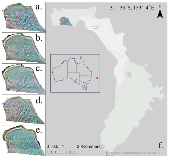
Figure 1.
Study location shown with red dot; North Bay, Lord Howe Island, and all collected orthomosaic maps; (a). November 2018; (b). March 2019; (c). May 2019; (d). September 2019; (e). November 2019; 31°33′S, 159°4′E; (f). Map of LHI, displaying North Bay in colour, and insert figure showing location in accordance with wider Australia.
2.2. Data Collection
Imagery was collected with a DJI Phantom 4 Pro drone, equipped with a high-resolution RGB camera (1″ CMOS with 20 M effective pixels and an 84° field of view), with an ND polarizing filter for imagery collection. Orthomosaic imagery was collected at an altitude of 50 m, with a front overlap of 75 m and a side overlap of 70 m, and across the entirety of North Bay, which spans ~700 m2. The resulting orthomosaic image was used for this study. The end result does not have any overlapping parts. The drone flew at a constant speed of 5 m/s. The program DroneDeploy was used for orthomosaic imagery collection and map building. All orthomosaic maps were built to a spatial resolution of 2 cm/px. A total of five orthomosaic maps were collected and produced across one year (November 2018, March 2019, May 2019, September 2019, and November 2019).
In situ video transects were undertaken during three mapping events, in May, September, and November 2019. Transects collected in May were used for ground truthing to inform drone-based OBIA image classification. All transects were used to provide additional information on the benthos of North Bay. Of these, five transects were collected in May and November, and three were collected in September (Figure 2). This discrepancy was due to logistical constraints. Transects were marked with a GPS and varied in location and depth across North Bay, chosen haphazardly within seagrass bed regions and deployed off mooring buoys within the reef flat region of the bay. The transects were all 50 m long. A tape measure was used in all video transects, and only sessile organisms and substrata directly under the transect were considered in the analysis. Video analysis benthos classifications included algae, sand, soft coral, hard coral, seagrass, and rubble/dead coral. Corals were assessed for growth form, size on a scale of from 1–5 (1: <5 cm, 2: 5–10 cm, 3: 10–20 cm, 4: 20–30 cm, 4: >30 cm), and bleaching on a scale of 1–9 (1. Normal, 2. Pale tops, 3. Pale, 4. Very pale tops, 5. Very pale, 6. Bleached tops, 7. Bleached, 8. Diseased, 9. Dead).
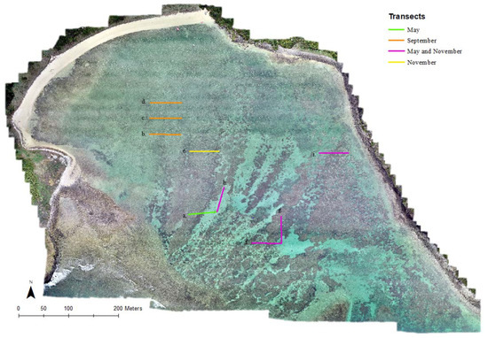
Figure 2.
Video transect locations across all months of sampling and associated transect number; a. May T4; b. Sep T1; c. Sep T2; d. Sep T3; e. Nov T2; f. May T1 and Nov T4; g. May T2 and Nov T3; h. May T3 and Nov T5; i. May T5 and Nov T1.
2.3. Developing Training Data using Object-Based Image Analysis
A convolutional filter was run on all orthomosaic images using ArcGIS Pro, to minimize differences in light among each orthomosaic in the time series. The orthomosaics were all clipped to a defined extent to allow for accurate comparisons to be made. One of the orthomosaic images was then chosen as a ‘training’ mask, to be classified semi-manually, using the program eCognition. This training mask covered the entirety of the bay (700 × 700 m), and all pixels containing corals, bleached corals, and instances of sun glint were identified and classified. eCognition provides a platform for classification using the object-based image analysis (OBIA) method. Firstly, a multi-resolution segmentation was run, using a scale parameter of 200, and defining composition criterion as shape: 0.2, and compactness: 0.3. This created large image objects, allowing for the classification of areas based on properties of spectral and textual similarity. To improve accuracy, classifications were then continued and altered manually. Finally, a further classification was then run on only ‘coral’ areas, using classified coral as super-objects on which a more refined image object classification was run to develop the class ‘bleached coral’. To improve accuracy, after the initial classification, this was then altered manually. A total of ten categories of classification were initially created, although this was reduced to four classifications (unbleached coral, bleached coral, sun glint, and background) for the final developed machine learning model (Supplementary Material Table S1). Mask accuracy was determined through ground truthing (Table 1) and validations run in GIS (Supplementary Material Table S2). Ground truthing was conducted based on the recorded in situ video transects, which were directly compared to the training data classifications using location. The process described in Section 2.3 can be found, explained as a schematic diagram, in Supplementary Material Figure S1.

Table 1.
Direct comparison validations between in situ transects (May) and OBIA mask classifications, developed based on March imagery.
2.4. Algorithm Pre-Processing
Orthomosaic imagery and mask classifications were tiled into smaller blocks for training to fit into standard memory and for faster processing. Images and masks were tiled into 4096 × 4096 px blocks, using the gdal2tiles package of the GDAL library. The 256 × 256 tiles were randomly assigned to each dataset, with 80% of tiles used for training, 10% for validation, and 10% for testing [27]. The network was trained for a maximum of 100 epochs over the entire dataset, with a 5 epoch patience set in place to prevent overfitting.
2.5. Developing and Running a Multi-Resolution Neural Network (mRES-uNet)
The neural network was developed based on a multi-resolution U-Net architecture [28], and adapted from Giles et al. (2021). mRES-uNet contains many of the same features as a U-net architecture, including a symmetrical architecture consisting of an encoding and decoding length (Figure 3). The encoder learns features in the image through a series of convolutions and downsampling via max pooling operations (Figure 4). The decoder locates features in the image by upsampling the image via transposed convolutions, utilizing skip connections to concatenate maps from the corresponding layer in the encoder, recovering spatial information that was lost in downsampling (Figure 4) [28]. mRES-uNet architecture has replaced the simple 3 × 3 convolution blocks in a traditional U-Net architecture with a concatenation of differing numbers of convolutional layers (called MultiRes blocks), allowing the network to better learn features on different scales within the image. Skip connections of the U-net architecture are also replaced by Res paths, containing a series of convolutions designed to bridge semantic gaps between the maps early on in the encoder with the much more processed maps in the decoder (Figure 3) [28].
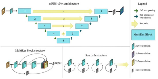
Figure 3.
mRES-uNet Architecture, including diagrams of the MultiRes block and Respaths. Adapted from [28].
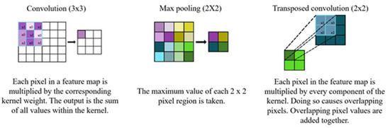
Figure 4.
Visual depictions of convolution, max pooling, and transposed convolution operations, including explanations [29,30,31,32].
For our network architecture, we use a 5-layer deep model while following the optimal MultiRes block hyperparameters experimentally determined by Ibtehaz and Rahman (2020) (Figure 3). Our resulting MultiRes blocks use filters [39, 79, 159, 319, 640] across levels, while our 4 Res paths contains filters [24, 48, 96, 192] along levels.
Our weighted cross-entropy loss function is given by Equation (1);
where and are the flattened ground truth and prediction vectors for the th class, respectively, and is the respective class weight.
The net (Equation (1)) consisted of four weighted classes; background, unbleached coral, bleached coral, and sun glint, where the weights are in place to mitigate the impact of class imbalances. The corresponding weights for these classes were; 1, 1.6, 5, and 5, respectively. The weights were determined experimentally in order to achieve the best total Jaccard scores with the coral and bleached coral classes. As Jaccard scores are not highly influenced by an imbalanced dataset such as ours (with only a small quantify of the objects of interest), we felt that this was a priority to achieve the most precise results. The Adam optimization algorithm was used during training, as per Giles et al. (2021).
2.6. Algorithm Training
The neural network took < 12 h for the model to train on Swinburne University’s OzStar Supercomputing Facility using one CPU core from an Intel 6140 Gold processor with 30 GB RAM and one GPU core from a NVIDIA P100 GPU (12 GB). The network was constructed in Python, using the Keras and TensorFlow packages [33,34]. The complete, trained model is freely available on GitHUB, using the URL https://github.com/daviesje/Full_Segmenter.
2.7. Building Temporal Robustness via Transfer Learning
In order to better account for deviations in lighting conditions from time differences, we fine-tuned our base net using a newly constructed dataset consisting of additional standardized small portions of orthomosaic imagery. This included three image tiles, each taken from three different orthomosaic images, collected in significantly different conditions. The training dataset for this process uses a portion of this dataset and contains a total of 429, 256 × 256 px tiles, with 75 tiles of these sampled randomly from our base training set of tiles. For the transfer learning process, we freeze the lowest 160 layers of our neural net and only allow the remaining high-level layers to update during the training process. This encourages the net to retain the generic features it has learned from the base model, while adapting to the specialized features given in this new, combined dataset.
2.8. Test of Model Performance
The testing of model performance utilizes the remaining tiles from the combined dataset of the other four orthomosaics and 33 tiles from the base validation set of tiles (total of 185, 256 × 256 px tiles). None of the chosen tiles had been used in any previous model training (Table 2).
Table 2.
Jaccard index, precision, and recall of neural network classifications.
2.9. Object-Based Bleached Coral Analysis
In addition to pixel-by-pixel analysis, bleached coral precision was also measured using an additional technique we have developed, the ‘object-based bleached coral analysis’ technique. This involves identifying a conglomerate of pixels that make up each individual bleached coral, with the intention of determining not only the percentage of bleached coral, but also the number of individual bleached corals within the entire area we assessed. Bleached corals were considered distinct, as long as they maintained a separation of at least one pixel across the entirety of its borders. This object-based approach prevented the counting of stray pixels, only considering bleached coral instances where there was >16 total pixel count in both the predicted map and the mask. Any pixel overlap between the two images (training mask and predicted map) would be considered a match, where the neural network successively associates a bleached coral to the underlying mask. We use the measurement of the overlap between the two images as another metric for model success.
3. Results
3.1. Mask Validations
Ground truthing in situ transects collected in May were used to validate the OBIA mask (based on immediate post-bleaching imagery collected in March). Transect information was simplified into the following classifications: coral, bleached coral, and background (sun glint excluded), for accurate comparisons. Validations revealed that 89.04% of mask classifications were correct. Transect one displayed the lowest accuracies (Table 1), likely due to a combination of the benthic complexity of this transect and potential GPS inaccuracies. We note that corals identified in transects as dead were classed in the category ‘coral’ in the OBIA mask, as they are no longer bleached, and are often covered in algae.
Manual validations of the original mask created by object-based image analysis were also performed through randomized visual inspection of pixels within five mask plot regions, conducted in GIS. This was undertaken to assess the accuracy of the semi-automatic workflow and to include sun glint in the validation process. Mask validations of each classification showed high levels of accuracy across classes, with sun glint presenting the highest levels of classification accuracy (99%), and bleached coral displaying the lowest classification accuracy (79%) (Supplementary Material Table S2).
3.2. Ground Truthing in Situ Transects
In situ transects provide ground truthing evidence for mask image classifications, along with additional information on the benthos of North Bay. May 2019 was characterized by a combination of sand (26.6%), rubble (27.6%), and hard corals (29.9%), with large areas of dead corals (Figure 5). No soft corals were recorded in transects in May (Figure 5). Transects in September 2019 were conducted in the shallower part of the bay, nearer to the beach, and were therefore largely made up of seagrass beds (44.0%) and sand (44.3%) (Figure 5). Transects in November 2019 covered the wide range of the bay, with sand covering 47.7% of transects, and hard corals also present in large amounts (26.1%) (Figure 5). Much of the recorded month to month variation is likely a result of differences in regions sampled, rather than any true major changes in composition (Figure 5). Of hard corals present across transects in May, September, and November 2019, corymbose and cespitose growth forms were the most common (Figure 6). A majority of corals were between 10 and 20 cm, regardless of date (Figure 6). Most >30 cm corals recorded were branching corals in large stands. Roughly half of the hard corals present in North Bay were healthy and unbleached (43.3, 50.0 and 36.1% for May, September, and November 2019, respectively) (Figure 6).
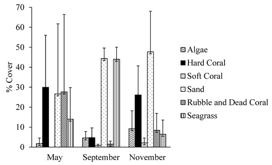
Figure 5.
Composition (%) of North Bay, Lord Howe Island, as recorded with in situ transects.
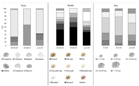
Figure 6.
Hard coral form, composition, and health, as recorded during in situ transects.
May 2019 displayed the largest variety of health statuses of hard corals and was the only date with diseased corals recorded. In September 2019, there were equal proportions of ‘pale tops’, ‘pale’, ‘very pale’, and ‘bleached’ tops corals (12.5% each), but no completely bleached hard corals were recorded. In November 2019, large quantities of bleached corals (25.9%) were recorded, along with lesser amounts of ‘pale’, ‘very pale’, and ‘dead’ corals (9.0, 8.6, and 8.2%, respective, Figure 6). All diseased corals recorded were branching corals, suffering from white band disease.
3.3. Neural Network Performance and Precision
The algorithm obtained an overall precision of 85.74% and an average Jaccard score of 0.56 across all classes on our test dataset. A Jaccard similarity index (given by TP/(TP + FN + FP), where TP is true positives, FN is false negatives, and FP is false positives) compares pixels from our predicted image and the underlying mask to determine similarity. Higher scores indicate a higher proportion of matching pixels compared to the total set of matching and mismatching pixels. High precision was achieved for unbleached coral and sun glint classifications (0.96 and 0.72, respectively), while bleached coral achieved a lower precision of 0.28 (Figure 7). Unbleached corals also obtained a high recall of 0.92, while sun glint obtained 0.53 and bleached coral 0.58 (Table 3). A Jaccard index was also determined for each class, finding relatively modest values for bleached coral and sun glint (0.23 and 0.44, respectively). Unbleached corals performed well, with a Jaccard score of 0.89 (Table 2).
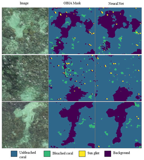
Figure 7.
Comparative classification of imagery with OBIA training mask and neural network.
Table 3.
Neural network confusion matrix of predicted values as % of true class, with diagonals highlighted in grey representing recall values.
3.4. Object-Based Bleached Coral Analysis and Precision
Due to the low accuracies of bleached coral, a further index was created to specifically test model performance for bleached corals, based on objects rather than pixels. This index could also potentially provide another useful measure for the assessment of coral abundance due to its ability to count colonies rather than pixels. The object-based bleached coral analysis predicted 44,339 individual bleached corals present in the March 2019 orthomosaic image, according to the OBIA classification training mask. Comparatively, the object-based bleached coral analysis prediction of the neural network classified image of March was 76,327 bleached corals. This results in an overall precision of 58%. This improved in areas with large numbers of bleached corals, such that tiles containing >1000 bleached corals resulted in a prediction precision of 0.66, and >2000 resulted in a prediction precision of 0.72. These significant improvements are the result of a removal of noise, in the form of other regions of the bay with similar characteristics as bleached corals, such as the beach.
Analysis of areas of low performance reveals that most errors were due to misclassified areas of land or shallow water dominated by sand, both of which are devoid of corals. Therefore, another analysis of performance was executed after the removal of land and sandy areas, resulting in a precision of 0.71 for regions with >1000 bleached corals, and tiles with >2000 bleached corals revealing a precision of 0.76. When run on all other orthomosaics, this analysis predicted 53,150 bleached coral colonies in November 2018, 57,481 in May 2019, 544,539 in September 2019, and 35,050 in November 2019. While these results generally appear as expected and suggest model effectiveness, the predicted amount of bleached coral colonies in September 2019 was disproportionately large and unexpected. Visual analysis of the classified regions reveals that this error was due to large areas of seagrass decline, leaving behind patchy light regions that were mistakenly identified as bleached coral by the algorithm (Figure 1). This highlights how the code can classify bleached corals in known coral dense regions with accurate and usable measurements, rather than places with a mixture of seagrass, sediments, and reefs.
3.5. Neural Network Classification Results
Background imagery (e.g., sand and seagrass) accounted for approximately half of the classified imagery during November 2018, May 2019, and November 2019, but was substantially more than half in March 2019 and less in September 2019 (Table 4). Aside from background, the classification of unbleached corals was dominant in all months of testing, although March 2019 recorded significantly less unbleached corals than all other months. Bleached corals were the most prominent in September 2019, accounting for 6.98% of the orthomosaic map, while March 2019 contained 2.21% bleached corals, and November 2018 contained 1.56% (Table 4). Both May and November 2019 were classified with <1% bleached corals. Accuracies for the classifications below were determined based on the 10% of imagery reserved for validation.
Table 4.
Results of % benthos classifications across all months of sampling.
4. Discussion
Coral reefs are threatened by the environmental stressors associated with anthropogenic climate change [35]. Cost-effective monitoring and assessment of these ecosystems is an important component of coral reef conservation strategies [7,36]. Small drones and computer vision can be combined to offer high resolution information on the abundance of corals and the extent of coral bleaching in such reefs, at scales less than 10 km2. Here, we developed a neural network to classify RGB drone imagery of coral reefs into unbleached and bleached corals, along with the additional classification of sun glint and background pixels. We achieved high precision and recall for the classification of unbleached corals (0.96 and 0.92) (Table 2 and Table 3). We also developed an object-based classification of bleached corals (Section 2.9) to improve accuracies for bleached coral classification, achieving up to 76% precision, along with the ability to provide a count of individual coral colony bleaching. These high resolution spatial and temporal accuracies present opportunities for automated and continual classification of our study site, to better inform managers of reef health. We contend that this freely available and fully trained algorithm, based on the latest image classification neural network, the mRES-uNet, can be a useful tool in monitoring small, shallow water reef systems worldwide, particularly when run on coral-dense imagery.
Deep learning algorithms trained on drone-based imagery present great possibilities for the automation of coral reef monitoring. The final model developed in the present study for assessing bleached and unbleached corals was a four-class mRES-uNet model (Figure 3) [28]. This model was developed as a progression of the U-Net architecture, a type of convolutional neural network (CNN) recently considered the most effective for image segmentation and classification [37,38,39]. The mRES-uNet was developed to decrease discrepancy between encoder and decoder lengths through the development of Multi-Res blocks (see Methods). This change has particular significance for ‘noisy’ datasets, outliers, and classifications without clear boundaries, where this model was found to consistently outperform the U-net structure, requiring fewer epochs to achieve this [28]. For the purpose of benthic classification in shallow marine ecosystems, this improved model is ideal, as coral reef imagery mostly consists of classifications without clear boundaries, due to overlap and similarities between benthos classes, and the effect of water and light on imagery.
The analysis of coral reefs with aerial imagery is not a new concept, but with the advent of novel technologies, sensors, and algorithms, there are new possibilities emerging for high resolution classification and monitoring [7,40]. Unbleached corals were able to be classified with very high levels of both precision and recall (Table 2 and Figure 7), which represent a strong agreement, according to Congalton and Green [41]. Therefore, it can be concluded that the developed methods are very effective for fast total coral cover estimates. Similarly, this has been achieved by a comparative study using random forest classifiers and RGB drone imagery to classify healthy corals, with similar results [42]. Drones have also been used to classify regions of unbleached corals and rubble in the Maldives, using OBIA for classification and health comparisons [15]. The present study combines such techniques, employing OBIA to develop a large-scale training dataset along with a deep learning algorithm to create an end-to-end coral classification tool able to account for subtleties of coral shape and disregard regions of dead, algae-covered coral and rubble.
Along with identifying regions of unbleached coral, we explored the possibilities of using RGB imagery and an image segmentation neural network to determine recovery from coral bleaching. To date, bleached and recovering coral colonies have not been successfully classified using aerial RGB drones and neural networks, although the use of underwater autonomous vehicles has been explored [20]. Here, regions of seagrass, algae-covered coral, and newly dead coral were originally included in our model (designed as a 6-class model), however due to non-descript borders and similarities between classes, these classifications were unable to be segmented with a high level of precision (Supplementary Material Table S1). Instead, greater focus was placed on the potential for classifying bleached corals. Initial bleached coral segmentation effectiveness indices indicated mixed performance, with a precision of 0.28 and a recall of 0.58 (Table 2). This implies that the model mislabeled other pixels as bleached coral (precision), but had relative success retrieving the complete set of bleached coral pixels (recall). This classification performed poorly when assessed by the Jaccard index of similarity, or IoU. However, this index is likely biased against such a dataset, as bleached coral only accounts for a very small percentage of image pixels, with large boundary proportions, which can skew this index [43]. As our dataset included unnecessary regions, such as areas of land or whitewash, which share characteristics with bleached coral, we suggest that image selection will be important for using our model with high resolution imagery, as it will drive improved precision [44].
As our network performed reasonably well for the recall of bleached corals, we developed an additional analysis, the object-based bleached coral analysis, as an added performance metric, with the ability to minimize precision inaccuracy. This algorithm clusters touching bleached coral pixels together to identify bleached coral colonies. Supervised object-based classification has become very popular for remote sensing applications [45]. However, unsupervised object classification is a newer field of study. A combined deep learning and OBIA strategy has been used on high-resolution satellite imagery for the classification of buildings, obtaining high levels of accuracy (>90%) [46], while an object-based CNN was tested on drone imagery for weed detection, leading to a precision of 0.65 and a recall of 0.68 [47]. Our results for bleached corals were comparable, although our object-based analysis was conducted post-pixel based neural network classification. When run only on regions with very high bleached coral density (with areas of sand and land removed), this method resulted in a precision of 76% bleached coral identification, as opposed to an overall 58% precision when run on the entire orthomosaic, including regions low in bleached corals (calculated as % of matched bleached coral colonies between the training mask and predicted map, see Methods). This represents a moderate agreement, according to Congalton and Green [41]. As satellite imagery, even at its highest resolution, is unable to determine individually bleached coral colonies, and crewed aircraft-based imagery fails to detect pale, along with completely bleached corals, the utility of our extra analysis is clear [48]. Furthermore, additional analyses prove that our model (both the ANN classification and object-based bleached coral analysis) will be more effective if run on coral dense imagery, and can be used to predict the total bleached coral colony count in such coral dense regions with high precision. This extends the use of our overall methodology, including not only pixel-based classifications, but an additional, highly accurate code to provide a count of bleached corals either across an entire orthomosaic or specific regions of interest.
While the combination of drone-based imagery and our model could facilitate the cost-effective monitoring of coral reefs, we suggest certain application strategies to gain the greatest accuracies. Firstly, we recommend the removal of unwanted regions of imagery, such as land, sand, or seagrass, as these can confound network classification. Additionally, temporal variation presents a significant problem for broad-scale accuracy, as not only can reef systems change significantly seasonally [49], but weather conditions, wind, tides, and general lighting conditions can also subtly alter images [50]. Such environmental influences can be mitigated with the expansion of training data to include more conditions. Our model was able to achieve high levels of precision temporally due to the inclusion of small trained regions of each image collected across the year. However, to expand the potential efficacy of this model temporally and to other similar reef systems, a small additional training dataset, or ‘labels’ from the period and area of interest, could be used to improve results. Such additional training data is not overly challenging, as it only needs to be a small section (e.g., 30 m2) of drone imagery, and image classification can be achieved manually or automatically, on GIS applications, object-based image analysis, or with the use of online resources [51]. Retraining and ‘fine tuning’ is a widely used step for computer vision projects [52]. As our network is already trained for coral reef classification, a small subsample of additional images is all that is necessary for achieving much greater accuracies. While the presented neural network is immediately useful to research aiming to classify unbleached corals and bleached corals in shallow reefs, through user interaction, this model could be expanded to many other shallow water coastal ecosystems, providing greater accuracies for specific tasks.
5. Conclusions
To facilitate the cost-effective monitoring of coral reefs, we developed an end-to-end model for the classification of unbleached and bleached corals, based on RGB drone imagery. We use a cutting-edge neural network, the mRES-uNet, to classify corals and include an object-based classification algorithm as an additional precision metric and to provide a count of individual bleached corals present. Overall, we have developed a model that can not only be immediately implemented for coral reef monitoring at Lord Howe Island, but can be easily adapted for monitoring other shallow water ecosystems. Accordingly, our model is freely available for use by researchers. We particularly encourage further interaction with it in the form of small sections of additional training data, so that it can better provide region and time-specific classifications. Drone imagery is ideal for rapid monitoring [53], but should be combined with in situ transects to capture both general large-scale change and fine-scale information. The combination of drone-based imagery and our novel model can facilitate cost-effective monitoring of small coral reefs worldwide, contributing to the conservation of these high-value ecosystems.
Supplementary Materials
The following supporting information can be downloaded at: https://www.mdpi.com/article/10.3390/rs15092238/s1, Table S1: 6-class neural network model with jaccard index, precision and recall. Corresponding weights for classes as follows: Background: 1, Sun glint: 5, Bleached Coral: 5, Newly Dead Coral: 2.4, Unbleached coral: 2, Seagrass: 1.2, Algae-covered coral: 1.2; Table S2: Mask classification validation accuracies; Figure S1: Schematic diagram describing the process of producing a training dataset using an object-based image analysis workflow.
Author Contributions
A.B.G.: conceptualization, methodology, formal analysis, writing—original draft, visualization; K.R.: software, formal analysis, writing—review and editing; J.E.D.: software, formal analysis, writing—review and editing; D.A.: formal analysis, writing—review and editing; B.K.: conceptualization, resources, writing—review and editing, supervision, funding acquisition. All authors have read and agreed to the published version of the manuscript.
Funding
Gear and software for this project were provided by ARC LIEF, Grant LE200100083. This work was also supported by the Holsworth Wildlife Research Endowment and the Ecological Society of Australia.
Data Availability Statement
All data created and used for this research is available by email request. Our code is available at https://github.com/daviesje/Full_Segmenter.
Acknowledgments
We would like to thank the team at Lord Howe Island Marine Park for the wonderful collaboration, particularly for help in collecting orthomosaic imagery and in situ transects. A special thanks to Sally-Ann Grudge, Caitlin Woods, Blake Thompson, and Justin Gilligan. This project would not have been possible without you.
Conflicts of Interest
The authors declare no conflict of interest.
References
- Anderson, K.; Gaston, K.J. Lightweight unmanned aerial vehicles will revolutionize spatial ecology. Front. Ecol. Environ. 2013, 11, 138–146. [Google Scholar] [CrossRef] [PubMed]
- Hughes, T.P.; Kerry, J.T.; Álvarez-Noriega, M.; Álvarez-Romero, J.G.; Anderson, K.D.; Baird, A.H.; Babcock, R.C.; Beger, M.; Bellwood, D.R.; Berkelmans, R.; et al. Global warming and recurrent mass bleaching of corals. Nature 2017, 543, 373–377. [Google Scholar] [CrossRef]
- Stuart-Smith, R.D.; Brown, C.J.; Ceccarelli, D.M.; Edgar, G.J. Ecosystem restructuring along the Great Barrier Reef following mass coral bleaching. Nature 2018, 560, 92–96. [Google Scholar] [CrossRef] [PubMed]
- Cantin, N.E.; Spalding, M. Detecting and Monitoring Coral Bleaching Events. In Coral Bleaching Ecological Studies; Springer: Cham, Switzerland, 2018; pp. 85–110. [Google Scholar] [CrossRef]
- Marshall, N.J.; A Kleine, D.; Dean, A.J. CoralWatch: Education, monitoring, and sustainability through citizen science. Front. Ecol. Environ. 2012, 10, 332–334. [Google Scholar] [CrossRef]
- Mumby, P.J.; Skirving, W.; Strong, A.E.; Hardy, J.T.; LeDrew, E.F.; Hochberg, E.J.; Stumpf, R.P.; David, L.T. Remote sensing of coral reefs and their physical environment. Mar. Pollut. Bull. 2004, 48, 219–228. [Google Scholar] [CrossRef]
- Hedley, J.D.; Roelfsema, C.M.; Chollett, I.; Harborne, A.R.; Heron, S.F.; Weeks, S.; Skirving, W.J.; Strong, A.E.; Eakin, C.M.; Christensen, T.R.L.; et al. Remote Sensing of Coral Reefs for Monitoring and Management: A Review. Remote Sens. 2016, 8, 118. [Google Scholar] [CrossRef]
- Scopélitis, J.; Andréfouët, S.; Phinn, S.; Arroyo, L.; Dalleau, M.; Cros, A.; Chabanet, P. The next step in shallow coral reef monitoring: Combining remote sensing and in situ approaches. Mar. Pollut. Bull. 2010, 60, 1956–1968. [Google Scholar] [CrossRef] [PubMed]
- Yamano, H.; Tamura, M. Detection limits of coral reef bleaching by satellite remote sensing: Simulation and data analysis. Remote Sens. Environ. 2004, 90, 86–103. [Google Scholar] [CrossRef]
- Joyce, K.E.; Duce, S.; Leahy, S.M.; Leon, J.; Maier, S.W. Principles and practice of acquiring drone-based image data in marine environments. Mar. Freshw. Res. 2019, 70, 952–963. [Google Scholar] [CrossRef]
- Koh, L.P.; Wich, S.A. Dawn of Drone Ecology: Low-Cost Autonomous Aerial Vehicles for Conservation. Trop. Conserv. Sci. 2012, 5, 121–132. [Google Scholar] [CrossRef]
- Alquezar, R.; Boyd, W. Development of rapid, cost effective coral survey techniques: Tools for management and conservation planning. J. Coast. Conserv. 2007, 11, 105–119. [Google Scholar] [CrossRef]
- Parsons, M.; Bratanov, D.; Gaston, K.J.; Gonzalez, F. UAVs, Hyperspectral Remote Sensing, and Machine Learning Revolutionizing Reef Monitoring. Sensors 2018, 18, 2026. [Google Scholar] [CrossRef]
- Teague, J.; Megson-Smith, D.A.; Allen, M.J.; Day, J.C.; Scott, T.B. A Review of Current and New Optical Techniques for Coral Monitoring. Oceans 2022, 3, 30–45. [Google Scholar] [CrossRef]
- Fallati, L.; Saponari, L.; Savini, A.; Marchese, F.; Corselli, C.; Galli, P. Multi-Temporal UAV Data and Object-Based Image Analysis (OBIA) for Estimation of Substrate Changes in a Post-Bleaching Scenario on a Maldivian Reef. Remote Sens. 2020, 12, 2093. [Google Scholar] [CrossRef]
- Levy, J.; Hunter, C.; Lukacazyk, T.; Franklin, E.C. Assessing the spatial distribution of coral bleaching using small unmanned aerial systems. Coral Reefs 2018, 37, 373–387. [Google Scholar] [CrossRef]
- Nababan, B.; Mastu, L.O.K.; Idris, N.H.; Panjaitan, J.P. Shallow-Water Benthic Habitat Mapping Using Drone with Object Based Image Analyses. Remote Sens. 2021, 13, 4452. [Google Scholar] [CrossRef]
- Collin, A.; Ramambason, C.; Pastol, Y.; Casella, E.; Rovere, A.; Thiault, L.; Espiau, B.; Siu, G.; Lerouvreur, F.; Nakamura, N.; et al. Very high resolution mapping of coral reef state using airborne bathymetric LiDAR surface-intensity and drone imagery. Int. J. Remote Sens. 2018, 39, 5676–5688. [Google Scholar] [CrossRef]
- Hamylton, S.M.; Zhou, Z.; Wang, L. What Can Artificial Intelligence Offer Coral Reef Managers? Front. Mar. Sci. 2020, 1049, 603829. [Google Scholar] [CrossRef]
- Jamil, S.; Rahman, M.; Haider, A. Bag of Features (BoF) Based Deep Learning Framework for Bleached Corals Detection. Big Data Cogn. Comput. 2021, 5, 53. [Google Scholar] [CrossRef]
- Dey, V.; Zhang, Y.; Zhong, M. A review on image segmentation techniques with remote sensing perspective. In Proceedings of the ISPRS TC VII Symposium—100 Years ISPRS, Vienna, Austria, 5–7 July 2010; Volume XXXVIII. [Google Scholar]
- Ghosh, S.; Das, N.; Das, I.; Maulik, U. Understanding Deep Learning Techniques for Image Segmentation. ACM Comput. Surv. 2019, 52, 1–35. [Google Scholar] [CrossRef]
- Harriott, V.; Harrison, P.; Banks, S. The coral communities of Lord Howe Island. Mar. Freshw. Res. 1995, 46, 457–465. [Google Scholar] [CrossRef]
- Valentine, J.P.; Edgar, G.J. Impacts of a population outbreak of the urchin Tripneustes gratilla amongst Lord Howe Island coral communities. Coral Reefs 2010, 29, 399–410. [Google Scholar] [CrossRef]
- Harrison, P.L.; Dalton, S.J.; Carroll, A.G. Extensive coral bleaching on the world’s southernmost coral reef at Lord Howe Island, Australia. Coral Reefs 2011, 30, 775. [Google Scholar] [CrossRef]
- NSW Government. Seascapes. Department of Primary Industries 2022. Available online: https://www.dpi.nsw.gov.au/fishing/marine-protected-areas/marine-parks/lord-howe-island-marine-park/life-under-the-sea/landscapes (accessed on 6 October 2021).
- Giles, A.B.; Davies, J.E.; Ren, K.; Kelaher, B. A deep learning algorithm to detect and classify sun glint from high-resolution aerial imagery over shallow marine environments. ISPRS J. Photogramm. Remote Sens. 2021, 181, 20–26. [Google Scholar] [CrossRef]
- Ibtehaz, N.; Rahman, M.S. MultiResUNet: Rethinking the U-Net architecture for multimodal biomedical image segmentation. Neural Netw. 2020, 121, 74–87. [Google Scholar] [CrossRef] [PubMed]
- Zhao, S. Demystify Transposed Convolutional Layers. Medium. 2020. Available online: https://medium.com/analytics-vidhya/demystify-transposed-convolutional-layers-6f7b61485454 (accessed on 6 October 2021).
- Shafkat, I. Intuitively Understanding Convolutions for Deep Learning. Towards Data Science. 2018. Available online: https://towardsdatascience.com/intuitively-understanding-convolutions-for-deep-learning-1f6f42faee1 (accessed on 11 October 2021).
- Powell, V. Image Kernels. Setosa. 2015. Available online: https://setosa.io/ev/image-kernels/ (accessed on 12 November 2021).
- Mishra, D. Transposed Convolutions Demystified. Towards Data Science. 2020. Available online: https://towardsdatascience.com/transposed-convolution-demystified-84ca81b4baba#:~:text=Transposed%20convolution%20is%20also%20known,upsample%20the%20input%20feature%20map (accessed on 6 October 2021).
- Abadi, M.; Agarwal, A.; Barham, P.; Brevdo, E.; Chen, Z.; Citro, C.; Corrado, G.S.; Davis, A.; Dean, J.; Devin, M. Tensorflow: Large-scale machine learning on heterogeneous distributed systems. arXiv 2016, arXiv:1603.04467. [Google Scholar]
- Chollet, F. Keras. 2015. Available online: https://keras.io (accessed on 26 December 2018).
- Hoegh-Guldberg, O. Coral reef ecosystems and anthropogenic climate change. Reg. Environ. Chang. 2011, 11, 215–227. [Google Scholar] [CrossRef]
- Bellwood, D.R.; Hughes, T.P.; Folke, C.; Nyström, M. Confronting the coral reef crisis. Nature 2004, 429, 827–833. [Google Scholar] [CrossRef]
- Alom, M.Z.; Hasan, M.; Yakopcic, C.; Taha, T.M.; Asari, V.K. Recurrent residual convolutional neural network based on u-net (r2u-net) for medical image segmentation. arXiv 2018, arXiv:1802.06955. [Google Scholar]
- Iglovikov, V.; Shvets, A. Ternausnet: U-net with vgg11 encoder pre-trained on imagenet for image segmentation. arXiv 2018, arXiv:1801.05746. [Google Scholar]
- Oktay, O.; Schlemper, J.; Folgoc, L.L.; Lee, M.; Heinrich, M.; Misawa, K.; Mori, K.; McDonagh, S.; Hammerla, N.Y.; Kainz, B. Attention u-net: Learning where to look for the pancreas. arXiv 2018, arXiv:1804.03999. [Google Scholar]
- Hamylton, S.M. Mapping coral reef environments: A review of historical methods, recent advances and future opportunities. Prog. Phys. Geogr. 2017, 41, 803–833. [Google Scholar] [CrossRef]
- Congalton, R.G.; Green, K. Assessing the Accuracy of Remotely Sensed Data: Principles and Practices; CRC Press: Boca Raton, FL, USA, 2019; Available online: https://books.google.com.ec/books?hl=es&lr=&id=yTmDDwAAQBAJ&oi=fnd&pg=PP1&ots=1HaQilihig&sig=hfe0btykmLoM6xWds0y0mqZebIU&redir_esc=y#v=onepage&q&f=false (accessed on 10 April 2023).
- Bennett, M.K.; Younes, N.; Joyce, K.E. Automating Drone Image Processing to Map Coral Reef Substrates Using Google Earth Engine. Drones 2020, 4, 50. [Google Scholar] [CrossRef]
- Cheng, B.; Girshick, R.; Dollár, P.; Berg, A.C.; Kirillov, A. Boundary IoU: Improving object-centric image segmentation evaluation. In Proceedings of the IEEE/CVF Conference on Computer Vision and Pattern Recognition 2021, Nashville, TN, USA, 20–25 June 2021; pp. 15334–15342. [Google Scholar]
- Ammour, N.; Alhichri, H.; Bazi, Y.; Ben Jdira, B.; Alajlan, N.; Zuair, M. Deep Learning Approach for Car Detection in UAV Imagery. Remote Sens. 2017, 9, 312. [Google Scholar] [CrossRef]
- Ma, L.; Li, M.; Ma, X.; Cheng, L.; Du, P.; Liu, Y. A review of supervised object-based land-cover image classification. ISPRS J. Photogramm. Remote Sens. 2017, 130, 277–293. [Google Scholar] [CrossRef]
- Zhao, W.; Du, S.; Emery, W.J. Object-Based Convolutional Neural Network for High-Resolution Imagery Classification. IEEE J. Sel. Top. Appl. Earth Obs. Remote Sens. 2017, 10, 3386–3396. [Google Scholar] [CrossRef]
- Veeranampalayam, S.; Arun, N.; Li, J.; Scott, S.; Psota, E.; Jhala, J.A.; Luck, J.D.; Shi, Y. Comparison of Object Detection and Patch-Based Classification Deep Learning Models on Mid- to Late-Season Weed Detection in UAV Imagery. Remote Sens. 2020, 12, 2136. [Google Scholar] [CrossRef]
- Andréfouët, S.; Berkelmans, R.; Odriozola, L.; Done, T.; Oliver, J.; Müller-Karger, F. Choosing the appropriate spatial resolution for monitoring coral bleaching events using remote sensing. Coral Reefs 2002, 21, 147–154. [Google Scholar] [CrossRef]
- Brown, B.E. Adaptations of Reef Corals to Physical Environmental Stress. In Advances in Marine Biology; Blaxter, J.H.S., Southward, A.J., Eds.; Academic Press: Cambridge, MA, USA, 1997; Volume 31, pp. 221–299. [Google Scholar] [CrossRef]
- Bhatnagar, S.; Gill, L.; Regan, S.; Waldren, S.; Ghosh, B. A nested drone-satellite approach to monitoring the ecological conditions of wetlands. ISPRS J. Photogramm. Remote Sens. 2021, 174, 151–165. [Google Scholar] [CrossRef]
- Majewski, J. Why Should You Label Your Own Data in Image Classification Experiments? Towards Data Science. 2021. Available online: https://towardsdatascience.com/why-should-you-label-your-own-data-in-image-classification-experiments-6b499c68773e (accessed on 11 October 2021).
- Tajbakhsh, N.; Shin, J.Y.; Gurudu, S.R.; Hurst, R.T.; Kendall, C.B.; Gotway, M.B.; Liang, J. Convolutional Neural Networks for Medical Image Analysis: Full Training or Fine Tuning? IEEE Trans. Med. Imaging 2016, 35, 1299–1312. [Google Scholar] [CrossRef]
- Jiménez López, J.; Mulero-Pázmány, M. Drones for Conservation in Protected Areas: Present and Future. Drones 2019, 3, 10. [Google Scholar] [CrossRef]


Disclaimer/Publisher’s Note: The statements, opinions and data contained in all publications are solely those of the individual author(s) and contributor(s) and not of MDPI and/or the editor(s). MDPI and/or the editor(s) disclaim responsibility for any injury to people or property resulting from any ideas, methods, instructions or products referred to in the content. |
© 2023 by the authors. Licensee MDPI, Basel, Switzerland. This article is an open access article distributed under the terms and conditions of the Creative Commons Attribution (CC BY) license (https://creativecommons.org/licenses/by/4.0/).