Article

Method of Validating Satellite Surface Reflectance Product Using Empirical Line Method

1
Department of Electrical Engineering and Computer Science, South Dakota State University, Brookings, SD 57007, USA
2
Imaging Center, Image Processing Laboratory, Department of Electrical Engineering and Computer Science, South Dakota State University, Brookings, SD 57007, USA
*
Author to whom correspondence should be addressed.
Remote Sens. 2023, 15(9), 2240; https://doi.org/10.3390/rs15092240
Submission received: 14 March 2023 / Revised: 18 April 2023 / Accepted: 21 April 2023 / Published: 23 April 2023

Abstract

:
Atmospherically corrected surface reflectance (SR) products are used for reliable monitoring of land surfaces and are the standard products of Landsat sensors. Due to increased demand for SR products, a need exists to verify that the L2C2 (Level-2 Collection-2) SR products are precise and accurate. The Level-2 Collection 2 (L2C2) SR Product has processed satellite imagery data that correct for atmospheric effects such as absorption and scattering, providing a more accurate representation of Earth’s surface. The validation of SR products using ground truth measurement is essential. This study aims to develop and evaluate a validation methodology for satellite SR products. Thus, the Empirical Line Method (ELM) is used here for atmospheric validation of remotely sensed data. Validation is performed using the SR derived from ELM tied to ground truth measurement. Absolute surface reflectance models of Algodones Dunes and the Salton Sea located in North America Sonoran Desert are developed to extend the temporally limited ground truth measurements. This model can give ground truth reflectance in any time frame independent of time constraints. The result of the absolute surface reflectance model of Algodones Dunes indicates that the model predicts the response of Algodones Dunes with an average accuracy of 0.0041 and precision of 0.0063 and gives ground measurements across all multispectral between 350 and 2500 nm. For the Salton Sea, the model predicts the response of the Salton Sea with mean absolute error (MAE) of 0.0035 and gives ground measurements across all multispectral between 350 and 2500 nm. The ELM generates atmospheric coefficients (gain and bias), which are applied to an image to obtain SR. Validation results indicated that for L9-OLI-2, L8-OLI, and L5-TM-SR products, the RMSE range is 0.0019 to 0.0106, 0.0019 to 0.0148 and 0.0026 to 0.0045 reflectance unit, respectively, and accuracy is within 0.0038, 0.0022, and 0.0055 reflectance unit across all spectral bands of L9, L8, and L5, respectively. On average, the validation result showed a strong linear relation between the L2C2 SR products and ELM SR within 0.5 to 1 reflectance units. These results demonstrate the high accuracy and reliability of the L2C2 SR product, providing valuable information for a wide range of remote sensing applications, including land cover and land use mapping, vegetation monitoring, and climate change studies.

1. Introduction

1.1. Background

Satellite remote sensing has been a critical factor in monitoring and quantifying changes on Earth’s surface and atmosphere at a regional, continental, and global scale. For the various applications of remote sensing, such as land cover classification, crop change monitoring, water resource monitoring, and global change monitoring, surface reflectance (SR) plays an important role [1]. Landsat imagery SR products are provided by U.S. Geological Survey (USGS) and Earth Resources Observation and Science (EROS), known as a “higher-level” Landsat Level-2 Collection-2 Surface Reflectance (L2C2 SR) product. L2C2 SR product is generated by atmospherically correcting Level-1 Top-of-atmosphere reflectance (TOA), defined as the ratio of incoming solar radiation reflected from the ground to the sensor [SGS; http://earthexplorer.usgs.gov/ (4 August 2022)] and is used for the geographical study of land surfaces [2]. Due to increased demand for SR products, a need exists to verify that the USGS-generated L2C2 SR products are precise and accurate. However, several techniques for atmospherically correcting Level-1 TOA reflectance and validating L2C2 SR products have been developed in recent years using temporally limited ground truth measurements that have a finite spatial range [3]. Moreover, direct validation of L2 products becomes problematic due to insufficient surface measurements at enough sites. Therefore, the primary focus of this work is to develop an atmospheric correction technique for the validation of surface reflectance products that consists of temporally extended ground truth measurements by the absolute surface reflectance model. The model is independent of the time constraints and gives the ground truth measurement in all multispectral between 350 and 2500 nm wavelength going back and forth in time.

1.2. Literature Review

Previously, various techniques were developed, and analyses were performed to evaluate the quality and accuracy of L2C2 SR products. The Landsat Ecosystem Disturbance Adaptive Processing System (LEDAPS) algorithm was analyzed by different studies and compared with MODIS SR products, AERONET site, and a second simulation of the satellite signal in the solar spectrum (6S) [2,4,5]. As the LEDAPS works on Dark-Dense vegetative algorithm [6], the results shown in this paper were consistent over more vegetation and no nearby water areas, which is expected. However, weaker performance of LEDAPS was observed in shorter wavelength bands and non-vegetative areas [5]. Moe et al. validated the Landsat 8 OLI L2C2 SR products with near-synchronous measurements from 13 sites in the United States, Brazil, Chile, and France. Outcomes demonstrated good agreement between OLI L2C2 SR products and ground truth measurements, especially on the longer wavelengths over the bright and dark targets [7]. At the same time, weak performance was observed in shorter wavelength bands and sparsely vegetative areas [7]. Eric et al. evaluated the performance of Landsat 8 OLI L2C2 SR products by using an appropriate atmospheric correction algorithm, which was based on in-situ measurements of the atmospheric properties, by comparing with Moderate Resolution Imaging Spectroradiometer (MODIS) adjusted Bidirectional Reflectance Distribution Function (BRDF) products and by comparing with United States Surface Radiation Budget Network (US SURFRAD) measurements. The results demonstrated the higher accuracy of Landsat 8 OLI SR over Landsat 5/7 LEDAPS product. Pinto et al. evaluated the Landsat 8 OLI and Landsat 7 ETM+ L2C2 data using in-situ measurements from Turkey, Brazil, Chile, the United States, France, and Namibia. Results indicated a slightly improved Landsat-8 OLI SR in the longer wavelength bands and consistently decreased in the shorter wavelength bands. The result showed an OLI surface reflectance product improvement over all spectral bands familiar with the Landsat-7 ETM+ [8].
Validation techniques explained above are used to check the L2C2 SR product’s quality and accuracy based on several atmospheric methods, consisting of ground measurements and cross-comparison to other sensor SR products. Common approaches that have been proposed for atmospheric validation of satellite imagery includes image average or flat target normalization [9], dark pixel method [10], radiative transfer model such as 6S [11], LOWTRAN [12], MODTRAN [13], FLAASH [14] and ground calibration method such as Empirical Line Method [15,16]. Several authors have compared the effectiveness of these atmospheric correction techniques [17,18,19]. Even though the radiative transfer models frequently yield better results than other techniques, they require measured values of atmospheric parameters at the data acquisition time, which can be quite challenging while working with historical datasets. Normalization produces the poorest result, which does not require additional information. This implies that this specific normalization method may not be effective or may not yield accurate atmospheric correction results in the context of remote sensing or satellite imagery. The dark pixel method does not account for spatial variation in the atmosphere (entire scene correction), and true dark values rarely exist in an image. The alternative approach is Empirical Line Method (ELM) achieved to ground truth, which enables the straightforward calculation of surface reflectance if an invariant target exists or measurements of targets are available. Usually, the technique uses surfaces with varying albedo (dark and bright) [20]. The ELM needs ground truth reflectance measurements of various targets and can produce acceptable results. If the target is spectrally stable over time, the measurement must not be concurrent with data acquisitions [19].

1.3. Proposed Method of Atmospheric Correction and Validation

The main objective of this research is to validate L2C2 SR products by developing an atmospheric correction model. In this work, the ELM technique was employed for atmospheric correction of remotely sensed data from at-sensor digital numbers (DN) to ground reflectance. It is widely acknowledged as a precise, practical method for validating satellite imaging systems to transform multi-spectral and hyperspectral data from raw DNs to a surface reflectance factor [18,21]. The ELM approach has been used on relatively thin atmospheric layers primarily because it necessitates the identification of at least two homogenous targets with contrasting reflectance that is large enough to be resolved [21]. The ELM implies that two or more targets with various reflectance characteristics are present in an image, covering a wide range of reflectance values for the spectral bands measured by the sensor [22]. Using DN values measured by Landsat sensors and ground reflectance of two homogenous targets (bright and dark), the ELM method can generate atmospheric coefficients (gain and bias) for that specific location.
Firstly, two targets, Algodones Dunes as a bright target located in path 38/row 37 (p38r37), path 39/row 37 (p39r37) and the Salton Sea as a dark target located in path 39/row 37 (p39r37), were selected. The reason for selecting path 38 row 37 and path 39 row 37 is explained in the site selection section of the methodology. The absolute surface reflectance model was developed for both targets using L2C2 SR trends and ground measurements. This is an integral part of the methodology, as it is very challenging to have ground measurements for every satellite overpass. Therefore, based on a few ground measurements obtained for both targets, the absolute surface reflectance models were developed and explained in the Section 3. Then, the ELM method was implemented using L1C2 DN and absolute surface reflectance model data to estimate the atmospheric coefficients. These atmospheric coefficients (gain and bias) were then applied to an image to generate ELM surface reflectance (SR).
Secondly, SR products were validated against ELM surface reflectance for Landsat 8 L2C2 SR datasets and illustrated in Section 4. For the validation part, a pixel-level comparison was made between ELM SR and SR products from the region of interest (ROI) that included vegetation, water, dunes, and rocks of path 39 row 37. Additionally, Root Mean Square Error (RMSE), accuracy, and precision were computed between ELM SR and SR products to evaluate the performance of SR products. Furthermore, the developed methodology was applied in Landsat 9 and Landsat 5 surface reflectance to check the consistency of the ELM SR model. Lastly, pixel-level uncertainty analysis was performed using Monte Carlo simulation, which is explained in Section 3.
The structure of the paper is as follows. the first part provides an introduction to the project; the second part describes the data sources used; the third part describes the outline of the method and methodology; the fourth part describes the result and validation of different sensors and models; and the fifth section describes the discussion and conclusion.

2. Data Sources Overview

The data source overview section explains the data used to train the absolute surface reflectance model of Algodones dunes and the Salton Sea. The satellite image data came from the Landsat 8 OLI sensor specifying the L2C2 data [23], the ground truth data of the Algodones dunes came from the Analytical Spectral Device (ASD), and the hyperspectral reflectance image of the Salton Sea came from the Airborne Visible/Infrared Imaging Spectrometer (AVIRIS) [24]. Furthermore, the ELM SR model was applied to the data of Landsat 5 & 9 [23] to evaluate the SR products.

2.1. Landsat 9 OLI-2

Landsat 9 carries two scientific instruments, the Operational Land Imager (OLI-2) and a thermal infrared sensor (TIRS-2). The TIRS-2 sensor measures the thermal infrared radiation or heats that the Earth’s surface emits, and the visible, near-infrared, and short-wave infrared observations of the Earth’s surface are recorded by the OLI-2 sensor. Landsat 9 takes the position of Landsat 7 (launched in 1999) in orbit (8 days out of phase with Landsat 8). Landsat 9, like Landsat 8, has a higher imaging capacity than previous Landsat, enabling the addition of more critical data to the Landsat global land archive—around 1400 scenes every day. Landsat 9 collects and archives moderate-resolution reflective and emissive multi-spectral picture data for a minimum of five years to provide seasonal coverage of the worldwide land mass [25,26]. Landsat 9 L2C2 data was tested in this study. Landsat 9 SR product’s accuracy and precision were cross-validated with the SR from ELM.

2.2. Landsat 8 OLI

Landsat 8 carries two scientific instruments, the Operational Land Imager (OLI) and a thermal infrared sensor (TIRS). The TIRS sensor measures the thermal infrared radiation or heats that the Earth’s surface emits, and the visible, near-infrared, and short-wave infrared observations of the Earth’s surface are recorded by the OLI. Landsat 8 has 15-meter panchromatic, 100-meter thermal, and 30-meter multi-spectral spatial resolution and measures in the visible, near-infrared (NIR), and short-wave infrared (SWIR) sections of the electromagnetic spectrum. Landsat 8 traverses one earth orbit in 99 min. It repeats every 16 days, with an equatorial crossing time of 10:00 a.m. ±15 min. On the Worldwide Reference System-2 (WRS-2) path/row system, approximately 740 scenes are acquired per day, with a swath overlap (or side lap) ranging from 7% at the equator to approximately 85 percent at extreme latitudes [27]. Landsat 8 OLI sensor was used in this study for developing the absolute surface reflectance model of Algodones Dunes and the Salton Sea. Furthermore, Landsat 8 L2C2 SR data was validated with SR from ELM.

2.3. Landsat 5 TM

Landsat 5 carried two instruments Multi-Spectral Scanner (MSS) and the Thematic Mapper (TM). This satellite orbited the Earth in a sun-synchronous at 705 km (438 mi) and near-polar orbit. Every 99 min, Landsat 5 circled the Earth and had a 16-day cycle with an equatorial crossing time of 9:45 a.m. (±15 min). Landsat 5 TM was a whiskbroom-based multi-spectral mechanically scanning optical imager. Seven spectral bands, including the thermal band in the TM sensor, can be used in various applications such as global change, geology, oceanography, forestry, and agriculture. Visible bands [Band (1–5 and 7)] with a ground sampling pixel size of 30 m and thermal band [Band 6] with a ground sampling pixel size of 120 m [5,28]. Since the developed methodology is independent of time constraints, Landsat 5 TM sensor was used in this study to check this feature of methodology. Thus, the accuracy and precision of Landsat 5 L2C2 SR products were validated with ELM SR.

2.4. ASD

Analytical Spectral Device (ASD) is designed to collect faster, more precise spectral data for ground truth measurements. ASD can measure radiance, transmittance, reflectance, or irradiance in the spectrum region of 350 to 2500 nm wavelength. Before recording 2151 channels at specified wavelengths (350 to 2500 nm) at a 1 nm interval, ASD instruments resample the raw channels using cubic spline interpolation. To imitate nadir remote sensing settings, the ASD measurements were taken under direct solar illumination for the spectral range of 350 nm to 2500 nm, with the ASD radiometer positioned perpendicular to the samples. The designed scheme of ASD concerns acquiring Visible near-infrared (VNIR) and Short-wave Infrared (SWIR) spectra across a wide range of the electromagnetic spectrum [29]. For precise correlation to sensor data from satellites and aircraft, ASD field spectroradiometers produce high-quality field spectra at the necessary illumination and viewing geometry. A radiometric calibration of satellite images can be made using ground truth measurements produced by ASD devices. To generate a preliminary description of Algodones Dunes and primarily evaluate its intercalibration potential, a 4-day field campaign was carried out in March 2015 [30]. Due to its uniform spatial and temporal characteristics, the Algodones Dunes location was chosen as a desirable intercalibration site. An ASD spectroradiometer was used in this study to measure the hyperspectral reflectance from the Algodones Dunes. The reflectance obtained from this instrument was used as ground truth measurement that further helps to calibrate the surface reflectance model of Algodones Dunes to obtain absolute surface reflectance model.

2.5. AVIRIS

AVIRIS stands for “Airborne Visible/Infrared Imaging Spectrometer” and debuted on January 1, 1993. It is airborne-based equipment. AVIRIS is a one-of-a-kind optical sensor that delivers calibrated images of upwelling spectrum radiance in 224 contiguous spectral channels (bands) with wavelengths ranging from 380 to 2510 nanometers. The AVIRIS instrument has 224 detectors, each having a wavelength sensitivity range (also known as spectral bandwidth) of approximately 10 nanometers (nm), allowing it to cover the whole wavelength range between 380 and 2500 nm. To have hyperspectral measurements, the AVIRIS sensor was flown over the Salton Sea in a specific time of 2017 and 2019 that collects the hyperspectral measurements. The readings from the AVIRIS sensor can be converted to g. und reflectance data, which can subsequently be utilized for quantitative assessment of surface features, with suitable calibration and correction for atmospheric factors [31]. The ground truth measurement from the AVIRIS sensor was used to calibrate the surface model of Salton Sea to obtain absolute surface reflectance model.

3. Methodology

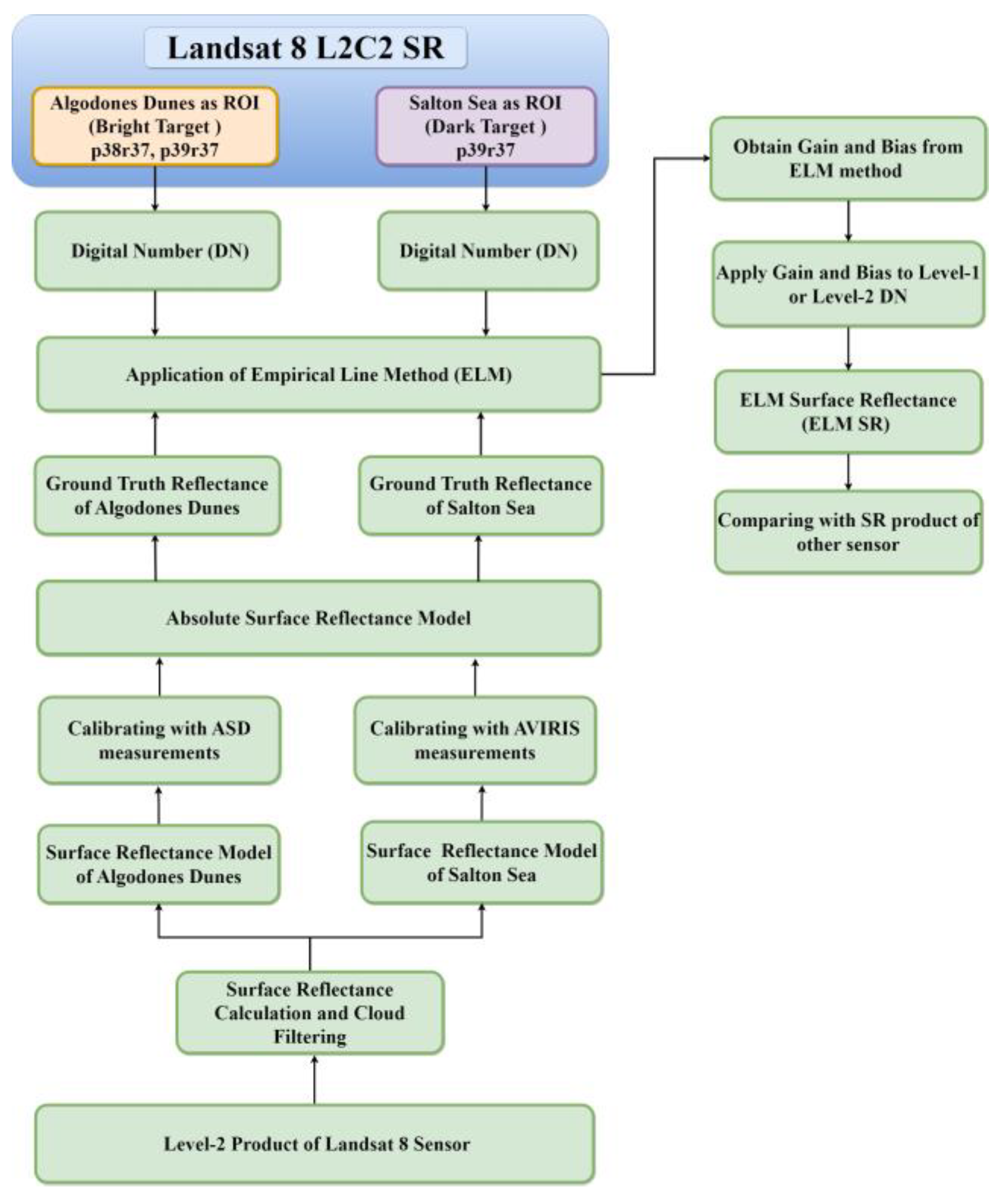
3.1. Method of Obtaining ELM Surface Reflectance

The main objective of this study was to develop and evaluate the suitable validation methodology for the SR product. Figure 1 shows the methodology used for producing SR by the ELM model. Initially, two sites were selected for developing the methodology, which is explained in site selection Section 3.1.1. Surface reflectance was calculated, and cloudy pixels were filtered out after selecting sites (see Section 3.1.2). Then a surface reflectance model was developed for both sites (Algodones Dunes and the Salton Sea), which predicts SR (see Section 3.1.3). The predicted surface reflectance model was tied/calibrated to ground measurements using ASD and AVIRIS data to obtain the absolute surface reflectance model (see Section 3.1.4). After that, Spectral Band Adjustment Factor (SBAF) was applied when validating the satellite other than Landsat 8 (see Section 3.1.4). The calibrated absolute surface reflectance model of two sites provides two inputs for the ELM model, and the remaining two inputs were L1C2 DN from the two sites. Later, the ELM technique was implemented based on the four inputs (see Section 3.1.5). Implementing the ELM model generates the atmospheric coefficients (gain and bias) based on the inputs. The obtained gain and bias, when applied to the L1C2 image gives surface reflectance, which is termed ELM surface reflectance (ELM SR).

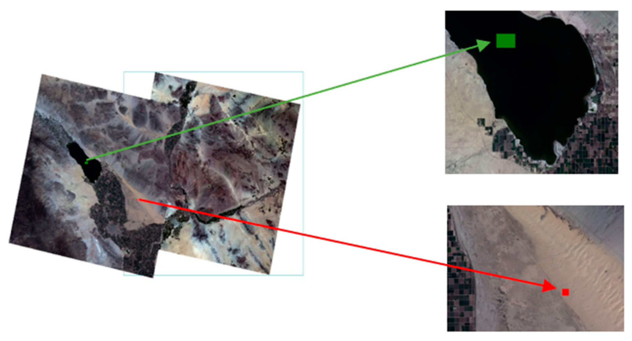
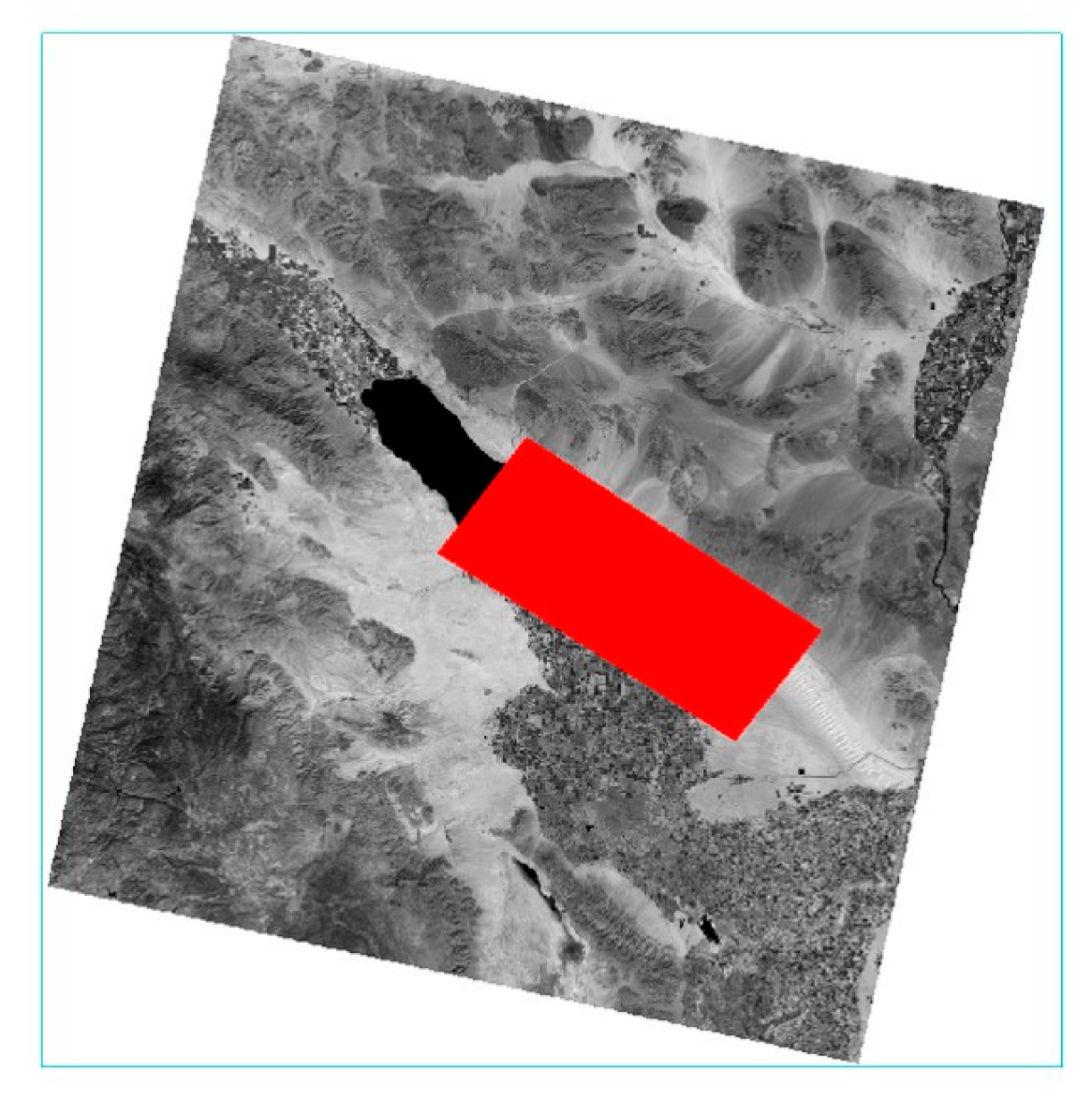
3.1.1. Site Selection and Region of Interest (ROI)

Since Algodones Dunes can be seen in both WRS-2 (World Reference System-2) path 39 row 37 and path 38 row 37, they were both selected to develop surface reflectance model of Algodones Dunes (bright target). The reason for selecting both paths and rows is to obtain more angle variation to assists a more robust model for Algodones Dunes. The Salton Sea (dark target) is located in Path 39 Row 37 only. Thus, only path 39 row 37 was selected for developing the surface reflectance model of Salton Sea. Algodones Dunes and Salton Sea ROIs as shown in Figure 2 were selected based on previous knowledge of the sites and available ground measurements from ASD [30] and AVIRIS (https://aviris.jpl.nasa.gov/ (9 July 2022)), allowing us to use them in an ELM development. The ground truth measurements were carried out in field sites that meet several criteria, including clear skies, high geographic homogeneity, and a low likelihood of atmospheric fluctuation. Implementing the ELM approach is challenging without surface measurements at the appropriate spatial, temporal, and spectral resolution for a given site. Ground truth reflectance is necessary at each acquisition for the selected ROI of path 39 Row 37. Therefore, a model must be developed to extend the limited ground truth measurements, to predict for dates whose ground truth is unavailable, via a time series analysis of data from Landsat 8.

3.1.2. Surface Reflectance Calculation and Cloud Filtering

For the development of an absolute surface reflectance model for Algodones Dunes and Salton Sea, a time series for each site is needed. Since Landsat 8 was chosen for this study, the image needs to be further converted from DN to reflectance using Equation (1) provided by the USGS.
ρ O L I , i = M U L D N i + A D D
where ρ O L I , i corresponds to surface reflectance values corresponding to band i; D N i is the digital number (pixel value) of Landsat 8 L2C2 SR product corresponding to a band i; MUL is the multiplicative scaling factor; and ADD the additive scaling factor used to convert DN to SR at band i. After the conversion of surface reflectance, a filtering process to remove clouds/shadows from the analysis was performed using the Quality Assessment (QA) Pixel band provided for Landsat 8 SR products. This process helps to remove outliers affected by clouds with measurements that do not represent the nature of the target and can lead to misleading results. The information in the QA band consists in the Bits that represent a combination of Dilated Cloud—Bits 1, Cirrus—Bits 2, Normal Cloud—Bits 3, Cloud Shadow—Bits 4, Cloud Confidence—Bits 9, Cloud Shadow Confidence—Bits 11, and Cirrus Confidence—Bits 15. To be used successfully, pixel values in the QA band must be converted into 16-bit binary form, and a cloud mask was created. Thus, the cloud-free image of Landsat 8 was obtained after applying a cloud mask.

3.1.3. Absolute Surface Reflectance Model for Algodones Dunes and Salton Sea

With Landsat 8 SR data, solar and sensor angles, the surface reflectance model of Algodones Dunes was developed. Afterward, the surface reflectance model of the Salton Sea was developed using the same process as Algodones Dunes with the addition of inherent properties of water. Lastly, both models were calibrated using ASD and AVIRIS ground measurements to develop an absolute surface reflectance model of Algodones Dunes and Salton Sea.
Development of Surface Reflectance Model for Algodones Dunes
Since most of the Earth’s surface is a non-Lambertian target, the surface reflectance of a given target can vary significantly depending on the sun’s illumination and the sensor’s observed geometry. Generally, the Bidirectional Reflectance Distribution Function (BRDF) can be used to model this effect. The surface reflectance model for the Algodones Dunes was developed using WRS-2, path 39 row 37, and path 38 and row 37 time series data since Algodones Dunes lies on both paths and rows. The dataset from two paths and rows assists in better model development due to more angle variation. The model was developed to predict the response of Algodones Dunes at any time during any acquisition.
This section explains usage of a four-angle, site-specific surface reflectance model for each band with minimal wavelength dependence [29]. The four-angle files, i.e., Solar Azimuth Angle (SAA), Solar Zenith Angle (SZA), View Azimuth Angle (VAA), and View Zenith Angle (VZA), were read from Landsat Archive. For further analysis, the spherical zenith and azimuth angles of the sun and the view zenith and azimuth angles of the sensor were converted to Cartesian coordinates. To preserve the nature of the data and MATLAB’s constraints in operating in a spherical coordinates system, a conversion to Cartesian coordinates was required [32]. The data was then mirrored to each quadrant to ensure symmetry with the scattering plane and a robust fit to the L8 surface reflectance data. Then, Equation (2) which represents a model for surface reflectance of sandy sites was fitted to the data.
ρ M o d e l = β 0 + β 1 X 1 + β 2 Y 1 + β 3 X 2 + β 4 Y 2 + β 5 X 1 Y 1 + β 6 X 1 X 2 + β 7 X 1 Y 2 + β 8 Y 1 X 2 + β 9 Y 1 Y 2 + β 10 X 2 Y 2 + β 11 X 1 2 + β 12 Y 1 2 + β 13 X 2 2 + β 14 Y 2 2
where β 0 , β 1 , β 14 coefficients were fitted to surface reflectance model of Algodones Dunes, which are least square coefficients of the model and are calculated with the known parameters X 1 , X 2 , Y 1 , Y 2 and reflectance, X 1 , X 2 , Y 1 , Y 2 represent the plane cartesian coordinate system converted from the spherical coordinate values (SAA, SZA, VAA, and VZA) using Equation (3). These least square coefficients of the model are used to predict the surface reflectance of Algodones dunes.
X 1 = sin ( SZA ) × sin ( SAA ) Y 1 = sin ( SZA ) × cos ( SAA ) X 2 = sin ( VZA ) × sin ( VAA ) Y 2 = sin ( VZA ) × cos ( VAA )
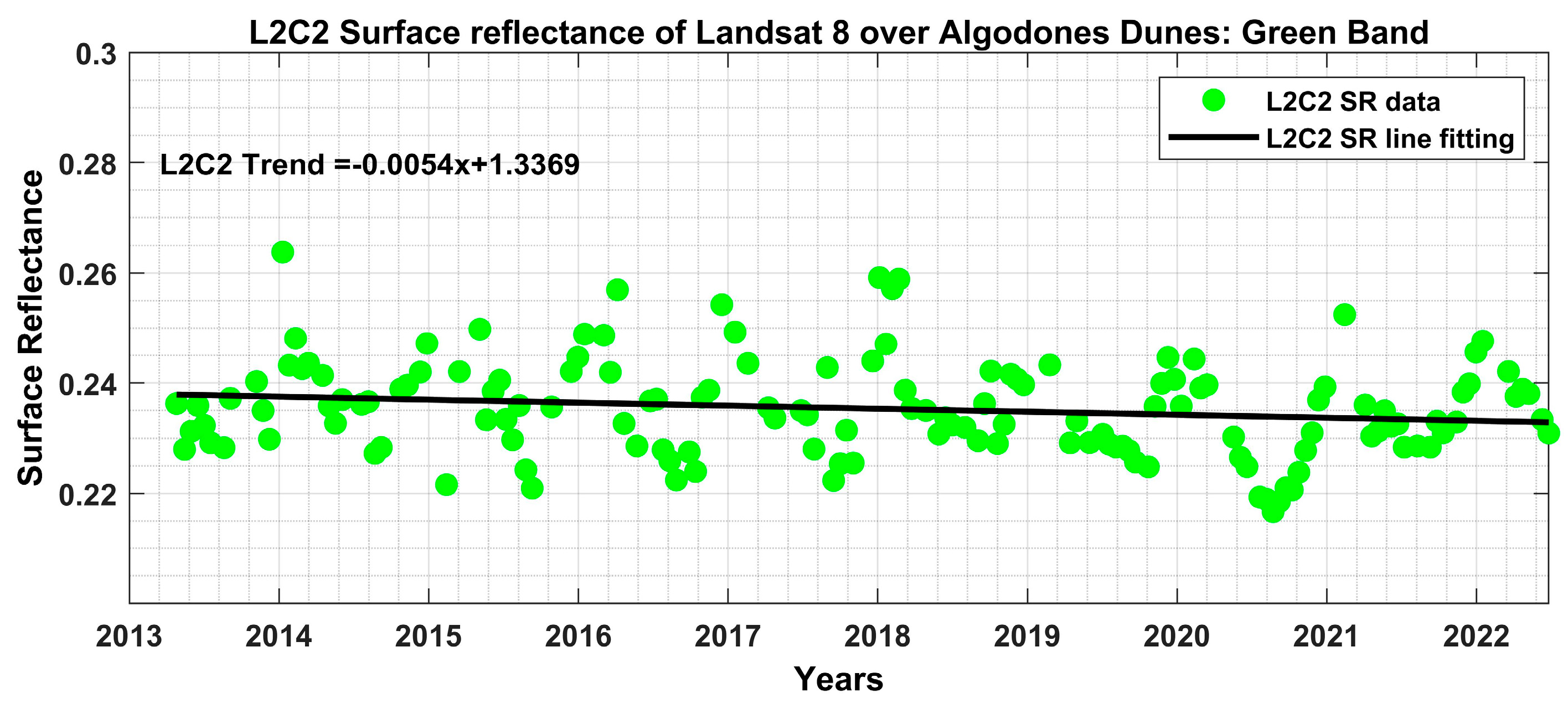
  • Trend Analysis of Algodones Dunes
During the development of the surface reflectance model for Algodones Dunes a decreasing negative trend was observed in the temporal dataset of the L2C2 SR product, as shown in Figure 3. For further understanding, this decreasing trend of surface reflectance model of Algodones Dunes must be investigated. The investigation is considered using only path 39 row 37.
The application of the ELM using bright and dark targets should be temporally, spectrally, and spatially modellable over a period of time; the decreasing trend of Algodones Dunes (bright target) must be investigated and corrected if necessary. Another ROI of Algodones Dunes (Optimal ROI of Algodones Dunes) was taken to investigate decreasing negative trend, and the temporal trend of L2C2 SR data was observed on that ROI. While observing the temporal trend of optimal ROI, the decreasing trend of L2C2 SR was observed of Algodones Dunes. Thus, after observing temporal L2C2 SR from two different regions of Algodones Dunes, the decreasing negative trend might be due to three reasons (i) there might be an issue with the atmospheric correction algorithm in L2C2 SR product by Landsat 8 sensor, (ii) the site, Algodones Dunes, might be changing over the time (iii) there might be an artifact in the sensor used for the analysis, which is Landsat 8 OLI. To address and determine which one represents the answer to the decreasing trend, the following approaches were taken for independently evaluating each option.
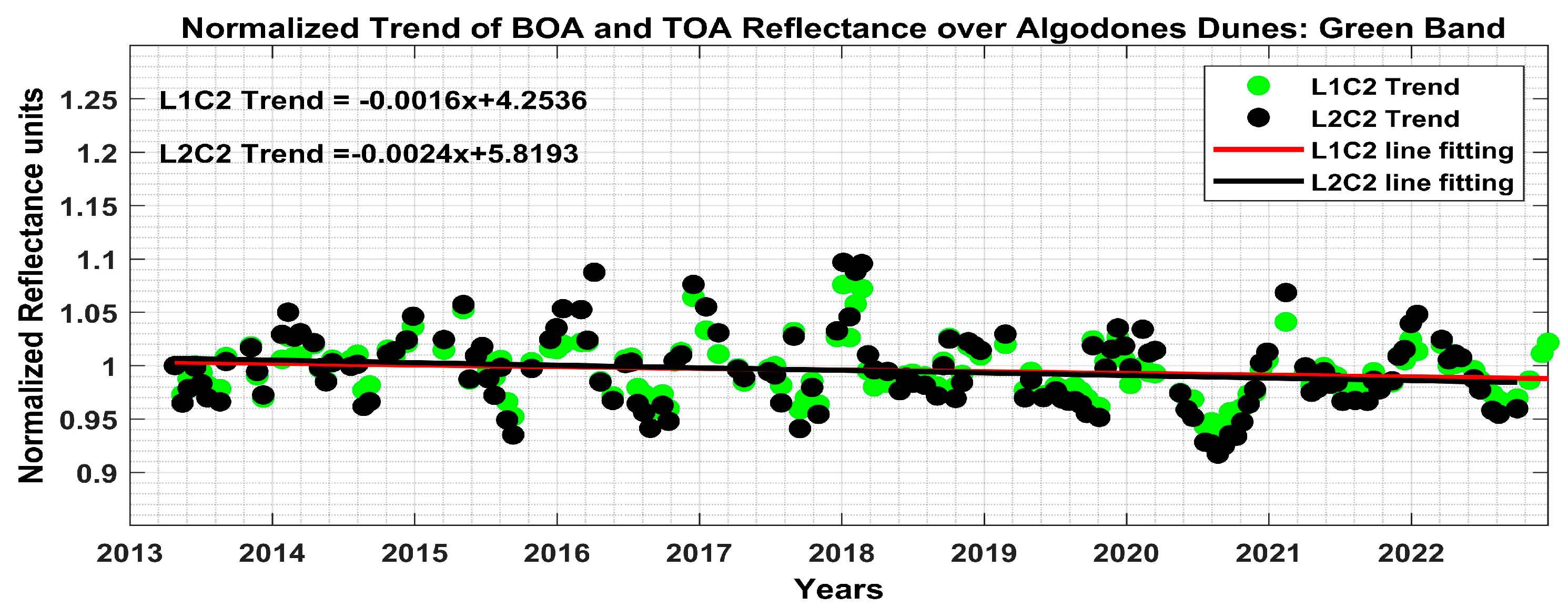
  • Investigation of atmospheric correction algorithm for L2C2 SR products: To see whether the decreasing negative trend was due to an issue with the atmospheric correction algorithm, the temporal trend of TOA L1C2 and Bottom of Atmosphere (BOA) L2C2 reflectance was observed for Algodones Dunes. To see a clear trend and pattern of both products, TOA and BOA reflectance were normalized at the first data point by dividing entire time series data with first data point of time series, and the normalized trend was obtained. While observing the normalized trend of TOA and BOA reflectance, as shown in Figure 4, both product trends and angular patterns follow each other where green dots represent the TOA L1C2 trend and black dots represent the BOA L2C2 trend. Again, the decreasing negative trend was observed in the temporal trend of BOA and TOA reflectance. This investigation shows that the decreasing negative trend was not due to an issue in the atmospheric correction algorithm of L2C2 SR products by Landsat 8 OLI sensor.
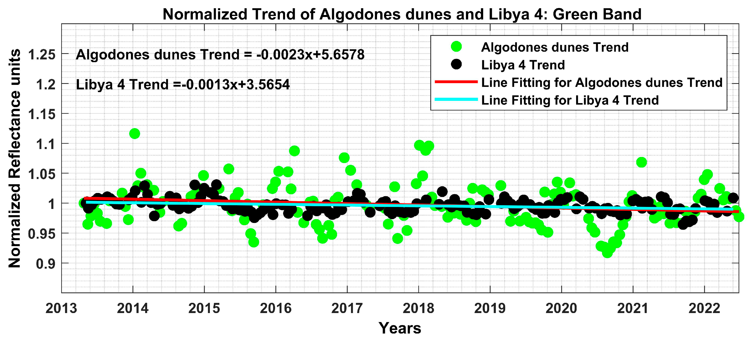
  • Investigation for the site might be changing: To see whether the decreasing negative trend was due to the changing site, another Pseudo Invariant Calibration site (PICS site) called Libya-4 from Path 181 Row 40 was taken into consideration. The Libya-4 is the PICS site, which is temporally, spectrally, and spatially stable over a period of time with relatively low uncertainties [29]. Figure 5 shows the normalized trend of Algodones dunes and Libya 4 by Landsat 8 where green dots represent the Algodones Dunes trend and black dots represent the Libya 4 trend. The decreasing negative trend was observed in the temporal trend of Libya-4 PICS, the same as of Algodones Dunes, as shown in Figure 5. It is nearly impossible for two sites in a different path and row to change at the same period, so this investigation shows that the negative decreasing trend was not due to the site. For further analysis, this investigation was extended to another satellite, i.e., Landsat 7 ETM+ for the Algodones Dunes.
  • Investigation for artifacts in the Landsat 8 OLI sensor used for analysis: To see whether the decreasing negative trend was due to artifacts in the Landsat 8 OLI sensor, another satellite was used to analyze Algodones Dunes. Landsat 7 ETM+ sensor was used for producing the temporal trend of L2C2 SR products for Algodones Dunes. Figure 6 demonstrates Landsat 8 & 7 normalized temporal trend of Algodones dunes, where green dots represent the L8 trend and black dots represent the L7 trend. While observing trends from Landsat 8 & 7, it’s uncertain that there is any decreasing negative trend in the Landsat 7 dataset of Algodones Dunes over Landsat 8. The Algodones Dunes seem to be stable without any trend over time. This investigation suggests that the decreasing negative trend might be due to the artifacts in the sensor.
For further analysis, this decreasing negative trend of Algodones Dunes was taken into consideration, and the surface reflectance model of Algodones Dunes was corrected with the same bias with which it was decreasing over time.
Development of Surface Reflectance Model for the Salton Sea
Furthermore, after developing the surface reflectance model of Algodones Dunes (Bright target), the surface reflectance model of Salton Sea (Dark target) was developed, as shown in Figure 7. The model was developed using WRS-2 path 39 row 37, considering the Salton Sea as ROI. Figure 7 also shows how the developed model of the Salton Sea was applied to the surface reflectance model to predict the response of SR for the entire Landsat 8 acquisition. Initially, Level-2 SR product from Landsat 8 sensor and Sun-Sensor geometry were used for estimating the SR of Salton Sea (ROI).
According to Lee’s 2011 [33], it was essential to produce sub-surface remote sensing reflectance to compute absorption and backscattering coefficients. The sub-surface remote sensing reflectance was calculated using Equation (4),
r r s = R r s 0.52 + 1.7 R r s
where R r s is remote sensing reflectance above the surface of water and r r s is sub-surface remote sensing reflectance. This sub-surface reflectance was used for retrieving the inherent optical property (IOP) of water. Thus, it was essential to convert the above remote sensing reflectance of water bodies to sub-surface remote sensing reflectance. According to Pope RM et al. [34], pure seawater has known quantities for its inherent optical properties (IOPs), which can be calculated using the Quasi- Analytical Algorithm (QAA) algorithm [33]. The absorption and backscattering coefficients of water were computed using QAA [35]. The above-surface remote sensing reflectance was entered into a series of QAA algorithms, which then output the IOPs for the absorption and backscattering coefficients. Consequently, QAA Algorithm was used to measure the absorption and backscatter indices of the Salton Sea. The surface reflectance of water bodies and IOP of water were fitted by the application of least square fit, which gives the free parameter of the surface reflectance model.
According to Pope RM et al. [34], for the application of least square fitting in this analysis, the BRDF model for water must be developed. A planetary surface with a calm body of water has a distinctive BRDF pattern. Generally, a natural body of water does not emit isotropic spectrum radiation [36]. The angular impacts of the water-leaving radiance must be considered for the precise measurement of spectral radiance or reflectance. One uses the BRDF model to determine how radiation or reflectance varies depending on direction. It relies on the geometry of the solar sensor, the optical characteristics, and the water composition. The model was developed to predict the response of the Salton Sea at any time during Landsat acquisitions.
Semi-empirical BRDF modeling was used in this analysis for water bodies based on physical models and free parameters. One of the main reasons for carrying semi-empirical BRDF modeling was that they could accurately explain the physical factor and predict the surface reflectance of water bodies. In this study, Lee’s 2011 [33] model was used for developing the surface reflectance model of the Salton Sea. Based on Landsat 8 data gathered from the Salton Sea, the BRDF model of water-leaving reflectance was examined. The L2C2 surface reflectance product from Landsat 8 OLI and the Inherent Optical Properties (IOP) of water were used to estimate the predicted surface reflectance of the Salton Sea. Equation (5) ( R r s (λ, Ω)) was used to characterize predicted surface reflectance over Salton Sea.
R r s ( λ ,   Ω ) = ( G 0 w ( Ω ) +   G 1 w ( Ω ) b b w λ k λ )   b b w λ k λ + ( G 0 p ( Ω ) +   G 1 p ( Ω ) b b p λ k λ )   b b p λ k λ
where G 0 w , G 1 w , G 0 p ,   G 1 p were free coefficients of the model, which are dependent on angular geometry and phase function but independent of absorption and backscattering coefficients or wavelengths. These free parameters of the model were derived by (least square fit) using remote-sensing reflectance. Ω is the sun-sensor angular geometry, a combination of solar zenith, sensor zenith, and relative azimuth angle above water, and k is the summation of absorption and backscattering coefficients calculated using Equation (6).
k = a + b b
where a is the absorption coefficient (m−1), b b (Inherent Optical Property) = backscattering coefficient (   b b w + b b p ), b b w , b b p are the backscattering coefficient of the water molecule and particles, respectively.
The bidirectional water-leaving radiance can be greatly impacted by bottom reflectance [37]. Hence, this investigation concentrated on optically deep waters where bottom reflectance has no significant influence. Free parameters in this model were, G 0 w , G 1 w , G 0 p ,   G 1 p which were retrieved for every sun-sensor geometry. Then, SR was predicted using these free parameters of the model.
Calibrating Surface Reflectance Model of Algodones Dunes and Salton Sea with ASD and AVIRIS Ground Reflectance Measurements
Model calibration was performed after developing the surface reflectance model of Algodones dunes and the Salton Sea. Model calibration was done with ground measurements taken from ASD and AVIRIS sensors over the sites. The calibration was done to make models in the modeling sector grounded to absolute via the ground truth measurements, which helps to develop an absolute surface reflectance model for both sites. Between model estimation and model application, model calibration takes place. Calibration was performed on the model once it had been estimated until it accurately reflected ground truth patterns and behavior. Figure 8 demonstrates the process of calibrating surface reflectance models of Algodones Dunes and the Salton Sea using ASD and AVIRIS ground measurements.
Due to the hyperspectral nature of ground truth observations, ground truth reflectance must be integrated to correspond to Landsat 8 multi-spectral bands [38]. By convolving the continuous ground truth reflectance with the Landsat 8 RSR function of the relevant OLI bands, it is possible to derive the multi-spectral reflectance of the ground truth measurements using Equation (7).
ρ G , i = λ 1 λ 2 ρ G λ . R S R i λ d λ λ 1 λ 2 R S R i λ d λ
where   ρ G ,   i   is the multi-spectral ground truth surface reflectance corresponding to a band i; R S R i λ is the OLI spectral response function of the corresponding bands; ρ G λ is the hyperspectral ground truth reflectance; and λ 1   λ 2 is the spectral range’s lower and upper wavelength in band i. The near-coincident date from the model and ground truth reflectance from ASD and AVIRIS sensors were used to compute the cross-calibration (cross-cal) factor using Equations (8) and (9). The process of cross-calibration is the transfer of a reference sensor’s calibration to a less well-calibrated sensor. This was accomplished by employing scene pairs obtained by two sensors that have a common ground target (coincident or near coincident).
C r o s s   c a l f a c t o r i f o r   S a l t o n   S e a = A V I R I S i S u r f a c e   r e f l e c t a n c e   m o d e l _ d a t a i
C r o s s   c a l f a c t o r i f o r   A l g o d o n e s   D u n e s = A S D i s u r f a c e   r e f l e c t a n c e   m o d e l _ d a t a i
where C r o s s   c a l f a c t o r i is the cross-cal factor for an ith particular date, s u r f a c e   r e f l e c t a n c e   m o d e l _ d a t a i is the surface reflectance data from surface reflectance model for ith date, A V I R I S i is the ground truth reflectance from AVIRIS for ith date, and A S D i is the ground truth reflectance from ASD for ith date. After taking the average of the cross-cal factors, multiplying the model data with the average cross-cal factor gives the absolute surface reflectance model of Algodones Dunes and Salton Sea. Thus, the absolute surface reflectance model of Algodones Dunes and Salton Sea was developed. The model was not limited to time constraints, which give ground measurement during Landsat acquisitions going back and forth in time.

3.1.4. Estimation of Spectral Band Adjustment Factor

The application of the absolute surface reflectance model of Algodones Dunes and the Salton Sea to other satellites, Spectral Band Adjustment Factor (SBAF), was implemented. SBAF is a compensating factor for matching the spectral response of two sensors [39] described in this section. Even when the satellite sensors used for the validation look at the same target through similar spectral regions, they respond differently in terms of spectral response. When validation is carried out, a systematic band offset may result from these variations in spectral response [40,41].
Landsat 5 TM, Landsat 9 OLI-2, and Landsat 8 OLI SR product validation were done in this work. As the absolute surface reflectance model was developed using Landsat 8 bands (model sensor), for the calculation of SBAF, the model sensor will always be Landsat 8. Another sensor was chosen as the reference sensor. To be validated, the spectral response should be adjusted using SBAF to match the response of the model sensor. The SBAF adjustment is given by Equation (10),
S B A F = ρ λ r e f ρ λ m o d e l = λ 1 λ 2 ρ λ h R S R λ r e f d λ λ 1 λ 2 R S R λ r e f d λ λ 1 λ 2 ρ λ h R S R λ m o d e l d λ λ 1 λ 2 R S R λ m o d e l d λ
where ρ λ r e f and ρ λ m o d e l are the simulated absolute surface reflectance model for the reference sensor and the model sensor; ρ λ h is the hyperspectral profile of the surface; and the R S R λ m o d e l and R S R λ r e f are the relative spectral response of the model sensor and the reference sensor, respectively. The λ 1 and λ 2 are upper and lower wavelength, respectively. The integration of the RSR of the multi-spectral sensor with the hyperspectral profile of the target at each sampled wavelength gives the simulated absolute surface reflectance model of the model sensor, as shown in Equation (10). The absolute surface reflectance model of the model sensor was converted to the corresponding absolute surface reflectance model of the model sensor using Equation (11).
ρ λ v a l = ρ λ   ×   SBAF
where ρ λ v a l is the absolute surface reflectance model of the reference sensor to be validated, which is equivalent to the absolute surface reflectance model of the model sensor, and ρ λ is the absolute surface reflectance model of the model sensor. While validating SR products of Landsat 9, and Landsat 5, the absolute surface reflectance models of the sensor to be validated was SBAF adjusted and were further used as inputs to the ELM for computing gain and bias.

3.1.5. Implementation of Empirical Line Method (ELM)

ELM was implemented after the development of absolute surface reflectance models or SBAF-adjusted absolute surface reflectance models of Algodones Dunes and the Salton Sea. The ELM is a technique that converts multi-spectral data from raw digital numbers (DNs) to at-surface reflectance factors by estimating atmospheric coefficients (gain and bias) [42]. The first target is PICS, a spatially, spectrally, and temporally stable site treated as the bright target. The second target is the reflectance observed over the water bodies, which usually have a low reflectance profile. The atmospheric coefficients (gain and bias) were calculated by the variation in reflectance unit of two targets. Empirically, it has been shown that linearity holds for the entire range of targets with low to high reflectance factors [43]. Assuming uniform atmospheric conditions around 50 miles radius of the ROIs, the atmospheric coefficients (gain and offset) can be applied to the image. There are four inputs for the computation of atmospheric coefficients (gain and bias) by ELM, and they are:
  • The DN value from the Algodones Dunes as ROI was the first input for the ELM. The DNs from Algodones Dunes were the higher value.
  • The DN value from the Salton Sea as ROI was the second input for the ELM. The DNs from the Salton Sea were the lower value.
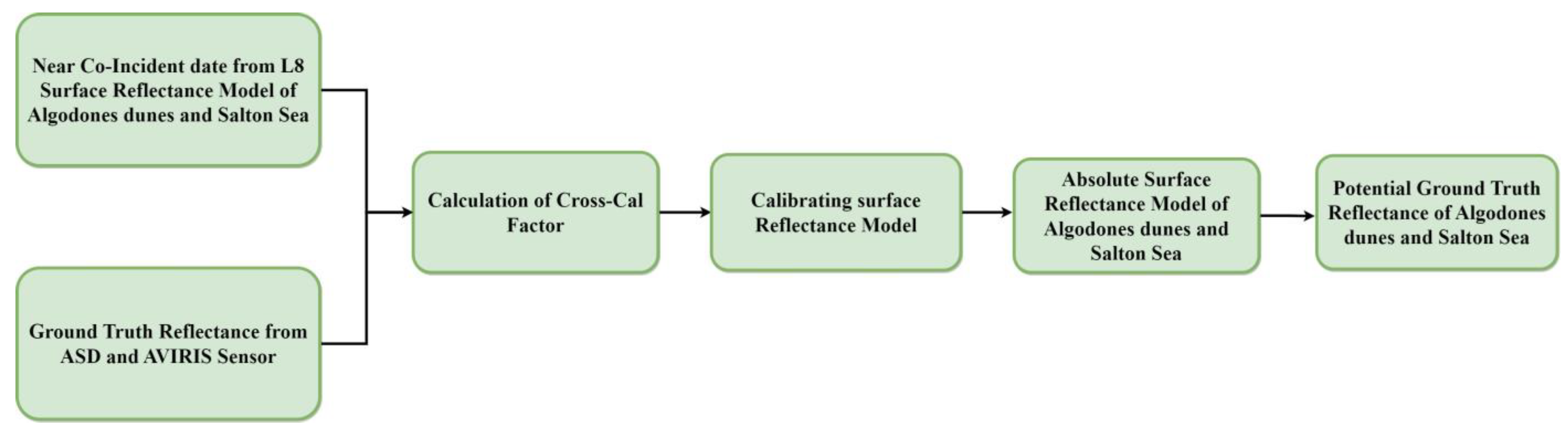
  • The absolute surface reflectance model of Algodones Dunes gave the ground truth reflectance of Algodones Dunes.
  • The absolute surface reflectance model of the Salton Sea gave the ground truth reflectance of the Salton Sea.

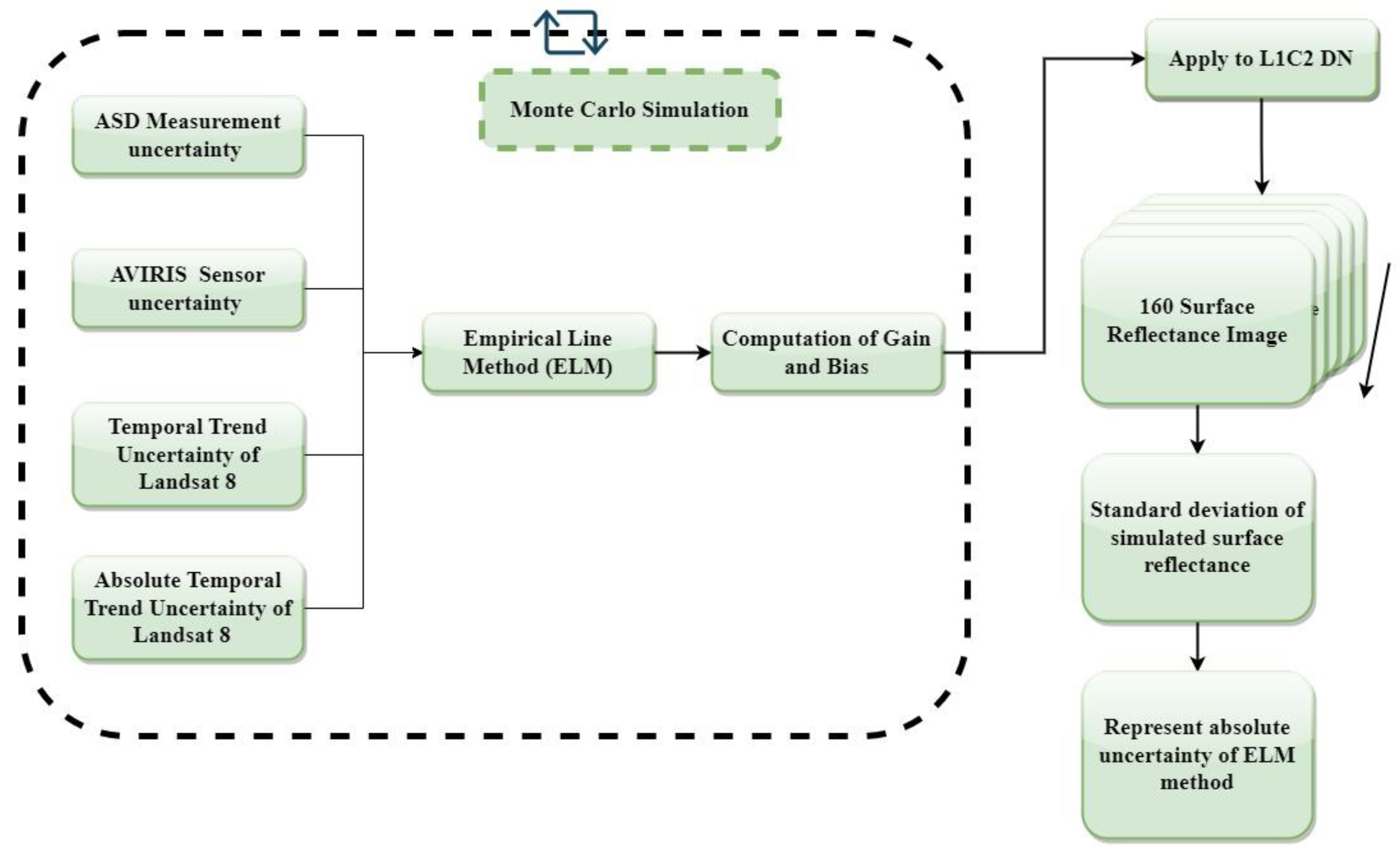
3.2. Uncertainty Analysis

Uncertainty analysis was carried out for ELM surface reflectance model using the Monte-Carlo Simulation method as shown in Figure 9. In short, Monte Carlo Simulation is a statistical method used to model and analyze systems by generating multiple random samples of input parameters, simulating scenarios, and estimating the probability of the outcomes. Monte-Carlo simulations for uncertainty propagation take as inputs the uncertainty distribution for each input parameter and equation for the estimative of the output uncertainty.
The rationale for proposing uncertainty analysis was to accurately assess the quality of ELM generated surface reflectance. For the application of the ELM method, four input parameters are required, as explained in Section 3.1. The four parameters are: (1) ASD measurements; (2) AVIRIS measurements; (3) a temporal trend associated with L8 SR product; and (4) absolute temporal trend associated with L8 SR product impact most for uncertainty calculation. Firstly, the uncertainty associated with these four parameters was calculated and obtained through a literature search, as presented in Table 1. The ASD uncertainty was estimated using repeatability. Repeatability assesses the reliability of the results and determine the uncertainty associated with the measurement. Repeatability is related to standard deviation of the measurements (see Equation (12)). Here, the ASD uncertainty ranges from 3.54% to 4.42% for all bands. According to Babu and Green et al. [44,45], the uncertainty associated with AVIRIS measurements was around ~8.6% for all bands. According to Barsi and Helder et al. [46,47], the uncertainty associated with the temporal and absolute temporal trend of L8 was within 2% for all bands.
ASD uncertainty = σ X ¯   ×   100 %
After obtaining the uncertainties associated with the input parameters of the ELM SR model, the ELM generates atmospheric coefficients (gain and bias) were calculated within their uncertainties using Monte-Carlo Simulation Method. To find the number of iterations for Monte-Carlo Simulation, the simulation started with 10 multivariate normal random numbers and calculated the pixel level total uncertainty for all bands. Then, simulation was continued up to 200 iteration levels by increasing 10 consecutive iterations. At 140 iterations, total uncertainty started to converge. Thus, by keeping the buffer of 20 iterations, 160 iteration levels were selected, and 160 gain and bias were calculated for further uncertainty analysis. Further, 160 simulated gain and bias were applied to the image, and 160 surface reflectance images were produced for all spectral bands. Finally, the standard deviation of 160 surface reflectance images gave the overall absolute pixel level uncertainty of the ELM SR model.

3.3. Data Evaluation and Comparison Methodology

After generating ELM SR products for Landsat 9, 8, and 5, there was a need for evaluation and comparison of L2 SR products. For Landsat 8, the L2C2 SR product was validated to ELM SR product. For Landsat 9 and 5, their corresponding SR products were cross-validated with ELM SR products. To compare ELM SR products with SR products, ROI was created of approximately a 50-mile radius near two calibration points. Figure 10 shows path 39 row 37, where the red box represents ROI, which covers Algodones dunes and Salton Sea (two calibration points) along with a variety of cover type. The atmospheric effect is assumed to be constant over ROI and used for pixel level comparison between ELM SR products and respective SR products. This ROI consists of almost 10 million pixels, so it will be challenging to compare pixel level between two products for the entire dataset of any sensors. To overcome this problem, a down-sampling process was performed where in each scene, pixels were down-sampled by 65 pixels.
After creating ROI, statistical metrics were calculated to evaluate the magnitude of agreement between both products.
  • Firstly, Root Mean Square Error (RMSE) was computed using Equation (13) between the ELM SR and respective SR products. The RMSE metric tells us how far apart the ELM SR values are on average from the L2 SR values in a dataset. The lower the model’s RMSE, the better it fits a dataset.
R M S E = i n y i y i 2 n
where y i represents the SR products value of each sample point (Pixel); y i is the ELM SR of each sample point, and n is the number of observations to be compared.
  • Secondly, accuracy and precision were calculated to see the absolute difference and variation between both products. Accuracy describes the method of average deviation between the ELM SR and SR products, using Equation (14). Precision describes the variation found in the respective band while measuring the same target repeatedly by the model using Equation (15).
A c c u r a c y = i n y i y i n
where y i represents the SR value of each sample point, y i is the ELM SR of each sample point, and n is the number os observations.
P r e c i s i o n = i n y i y i 2 n
where y i represents the SR value of each sample point, y i is the ELM SR of each sample point, and n is the number of observations.

4. Results

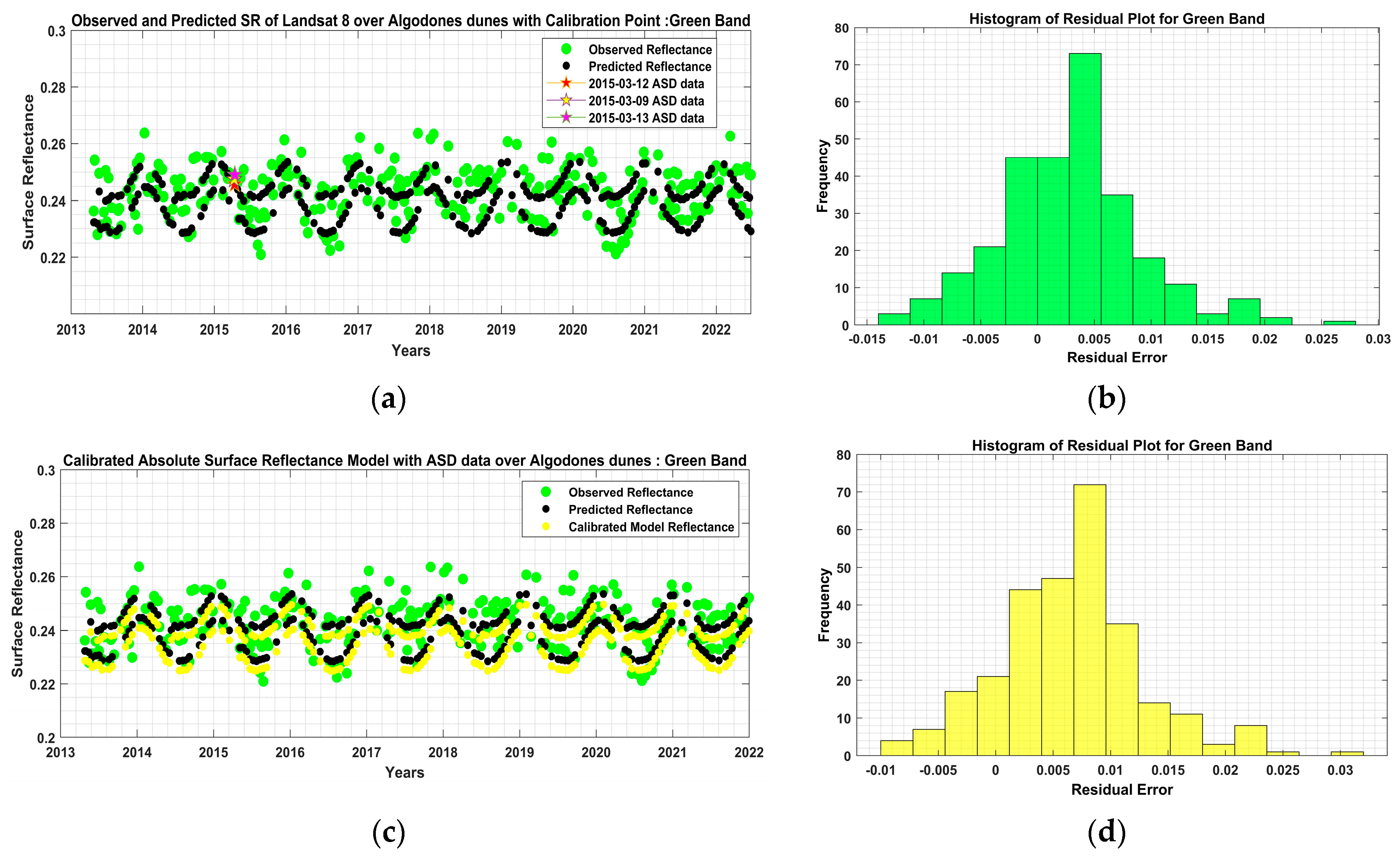
4.1. Evaluation of Absolute Surface Reflectance Model—Algodones Dunes

Figure 11a demonstrates that surface reflectance model predicted SR over Algodones Dunes for the green band. The green color represents observed Landsat 8 SR, and the black color represent predicted Landsat 8 SR for the entire Landsat 8 data acquisition. From Figure 11a, based on temporal variation, the surface reflectance model captured seasonal and angular variation of Landsat 8 observed reflectance quite well. The accuracy estimated at 0.0029 describes the average deviation between the surface reflectance model predicted SR and observed reflectance. The precision estimated at 0.0063 describes the variation found in the respective band while repeatedly measuring the same target by the surface reflectance model. After predicting the SR over Algodones Dunes by the surface reflectance model, the ground truth measurements by ASD were plotted, represented by red, yellow, and magenta dots. In Figure 11a, the ground truth measurements from ASD are lined up with the predicted SR by the surface reflectance model, further used for calibrating surface reflectance model of Algodones Dunes.
Figure 11b shows the histogram of residual error between the surface reflectance model’s predicted SR and observed reflectance in the green band. The histogram ranged from −0.015 to +0.03. The histogram plot indicates that the model works well within 0.015 of the residual error. However, the model is good within ± 0.01 as the majority of data intended to lie within this range.
After predicting the observed SR by surface reflectance model, the absolute surface reflectance model for Algodones Dunes was developed by calibrating with ASD measurements for three different dates represented by red, yellow, and magenta dots, as shown in Figure 11a. ASD measurements were spectrally integrated for the spectral response of all L8 Bands, and cross-cal factors were calculated. For the green bands, as shown in Figure 11a, three cross-cal factors are 0.995, 0.988, and 0.996. By taking the average of three cross-cal factors (0.993) and multiplying the surface reflectance model data gives the absolute surface reflectance model of Algodones Dunes.
Figure 11c represents a calibrated surface reflectance model, which leads to the absolute surface reflectance model of Algodones dunes. The yellow dots represent the calibrated absolute surface reflectance model of Algodones Dunes. The accuracy was estimated to be 0.0034, which describes the average deviation between the calibrated absolute surface reflectance model and L8 observed reflectance. The precision was estimated to be 0.0063, which describes the variation found in the respective band while measuring the same target repeatedly with the calibrated absolute surface reflectance model. The data from calibrated absolute surface reflectance model of Algodones Dunes were considered as ground truth data for the further analysis. Therefore, ground truth data from calibrated absolute surface reflectance model of Algodones Dunes were first input to the ELM method for obtaining surface reflectance.
Figure 11d shows the histogram of the residual error between the calibrated absolute surface reflectance model of Algodones Dunes and observed reflectance in the green band. The histogram ranged from −0.01 to +0.03. The histogram plot indicates that the calibrated absolute surface reflectance of Algodones Dunes works well within 0.01 of the residual error. However, the model is good within 0 to +0.012 as the majority of data intended to lie within this range.

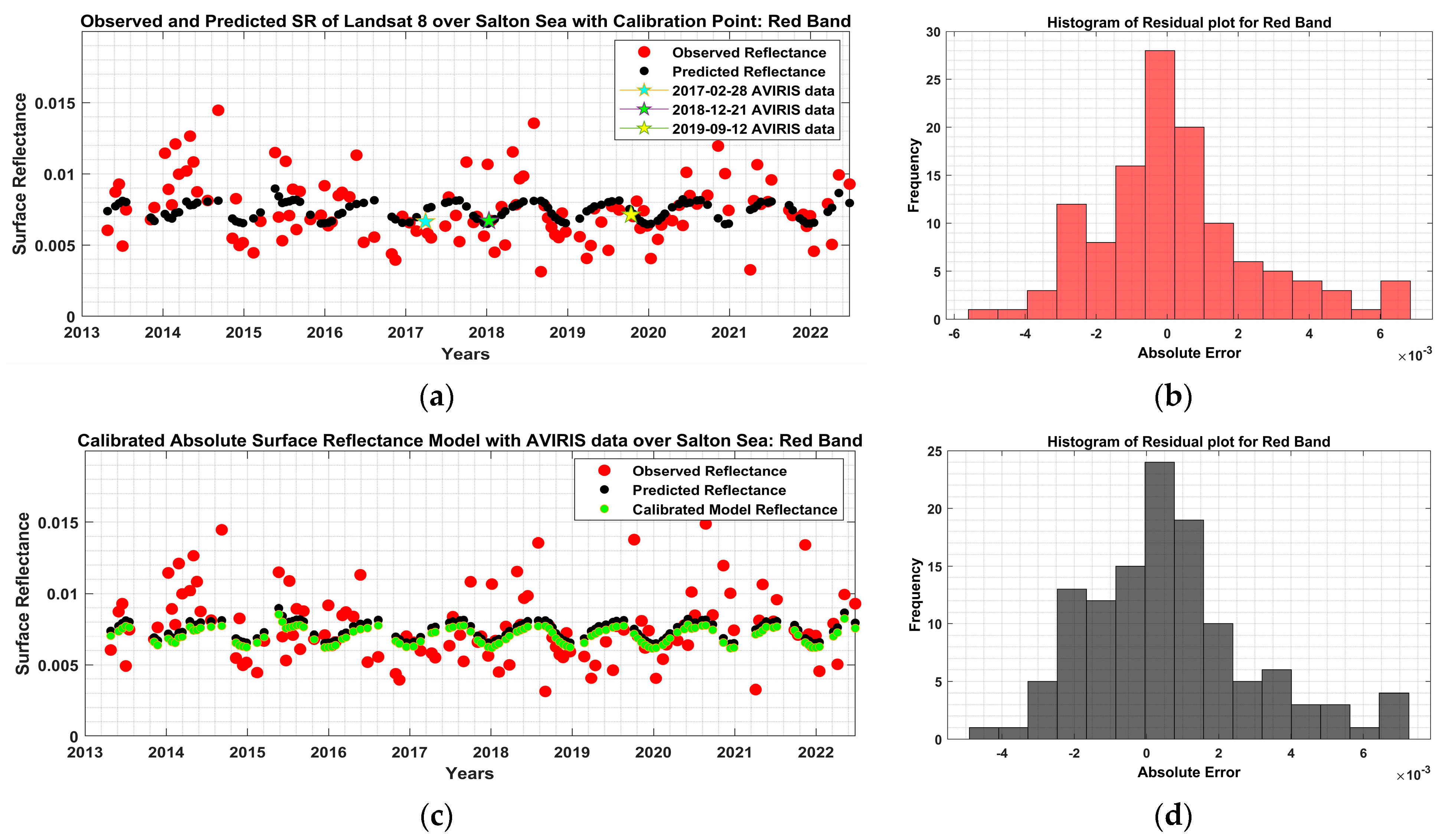
4.2. Evaluation of Absolute Surface Reflectance Model—Salton Sea

Figure 12a demonstrates the observed results and the surface reflectance model predicted SR over the Salton Sea for the red band. The red color represents observed Landsat 8 SR, and the black color represents predicted Landsat 8 SR for the entire Landsat 8 data acquisition. From Figure 12a, based on temporal variation, the surface reflectance model captured seasonal, and the angular variation of Landsat 8 observed reflectance quite well. The mean absolute error, estimated at 0.0015, describes the average deviation between the surface reflectance model predicted SR and observed reflectance. After predicting the SR over the Salton Sea via the surface reflectance model, the ground truth measurements by AVIRIS were plotted, represented by a pentagon shape of blue, green, and yellow dots. In Figure 12a, we can see that the ground truth measurements from AVIRIS are lined up with the predicted SR by the surface reflectance model, which was further used for calibrating surface reflectance model of the Salton Sea.
Figure 12b shows the histogram of absolute error between the surface reflectance model’s predicted SR and observed reflectance in the red band of the Salton Sea. The histogram ranged from −0.006 to +0.006. The histogram plot indicates that the model works well within 0.006 of the absolute error. However, the model is good within ± 0.004 as the majority of data intended to lie within this range.
Similar to the absolute surface reflectance model of Algodones dunes, the absolute surface reflectance model of Salton Sea was developed by calibrating Surface reflectance model using AVIRIS measurements of 3 different near-coincident dates. AVIRIS measurements of three dates are represented by a pentagon shape of blue, green, and yellow dots as shown in Figure 12a. AVIRIS measurements were spectrally integrated for the spectral response of all Landsat 8 Bands, and cross-cal factors were calculated. For the red bands as shown in Figure 12a, three cross-cal factors are 0.995, 0.988, and 1.004. By taking the average of three cross-cal factors (0.996) and multiplying the surface reflectance model datagives the absolute surface reflectance model of Salton Sea.
Figure 12c represents a calibrated surface reflectance model of the Salton Sea with AVIRIS measurements, which leads to the absolute surface reflectance model of the Salton Sea. The green dots represent the calibrated absolute surface reflectance model of the Salton Sea. The mean absolute error, estimated at 0.0017, describes the average deviation between the calibrated absolute surface reflectance model and observed reflectance. The data from calibrated absolute surface reflectance model of the Salton Sea were considered as ground truth data for the analysis. Therefore, ground truth data from calibrated absolute surface reflectance model of the Salton Sea were second input to the ELM method for obtaining surface reflectance.
Figure 12d shows the histogram of absolute error between the calibrated absolute surface reflectance model of the Salton Sea and the observed reflectance in the red band. The histogram ranged from −0.004 to +0.004. The histogram plot indicates that the calibrated absolute surface reflectance of the Salton Sea works well within 0.004 of the absolute error. However, the model is good within ± 0.003 as the majority of data intended to lie within this range.

4.3. Validation & Evaluation Results of Different Sensors SR Products

As explained in Section 3, to produce ELM SR, four input parameters are required. After performing all those analyses, we have four parameters: sensor measured DN’s value of Algodones Dunes and the Salton Sea, absolute surface reflectance model for both sites. After obtaining these values, the ELM was applied to calculate gain and bias, which were further applied to TOA reflectance products of Landsat 9, 8, and 5. This result for surface reflectance generated by the ELM SR model was based on the absolute surface reflectance model of Landsat 8. SR products from different sensors were validated and cross-validated with SR produced by the ELM SR model. Since the absolute surface reflectance model was based on Landsat 8 SR temporal trend, initially, Landsat 8 SR products were validated with SR generated by the ELM SR model presented in Section 4.3.1. In addition, the absolute surface reflectance model of Algodones Dunes & Salton Sea is independent of time constraints; the ELM SR model was used to validate Landsat 9 and 5 SR products going back and forth in time. Further, Section 4.3.2 shows the cross-validation results of Landsat 9 SR products, which means going forth in time, and in Section 4.3.3, the Landsat 5 SR product was cross-validated, which means going back in time to check the potential of absolute surface reflectance model of Algodones Dunes and Salton Sea.

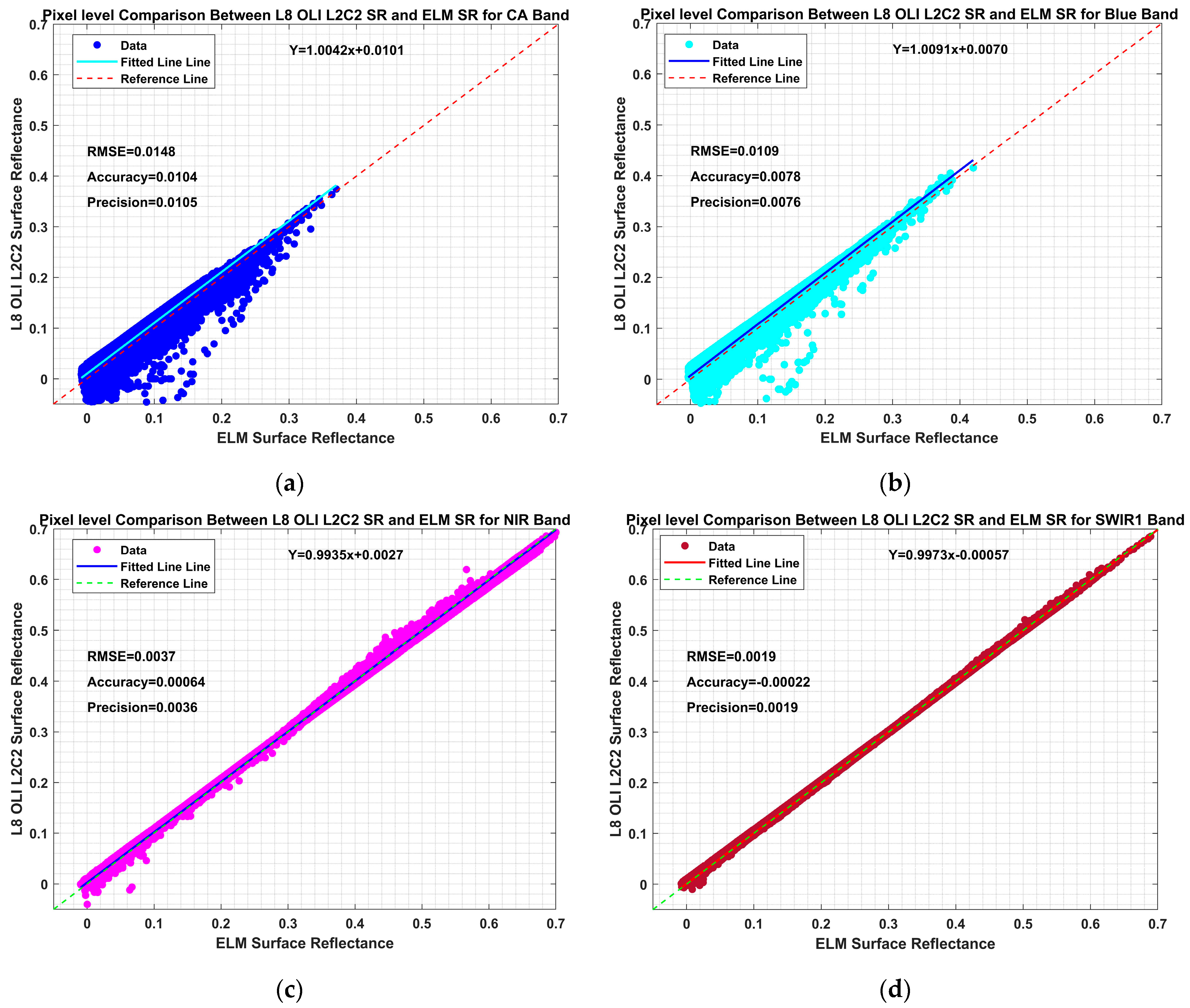
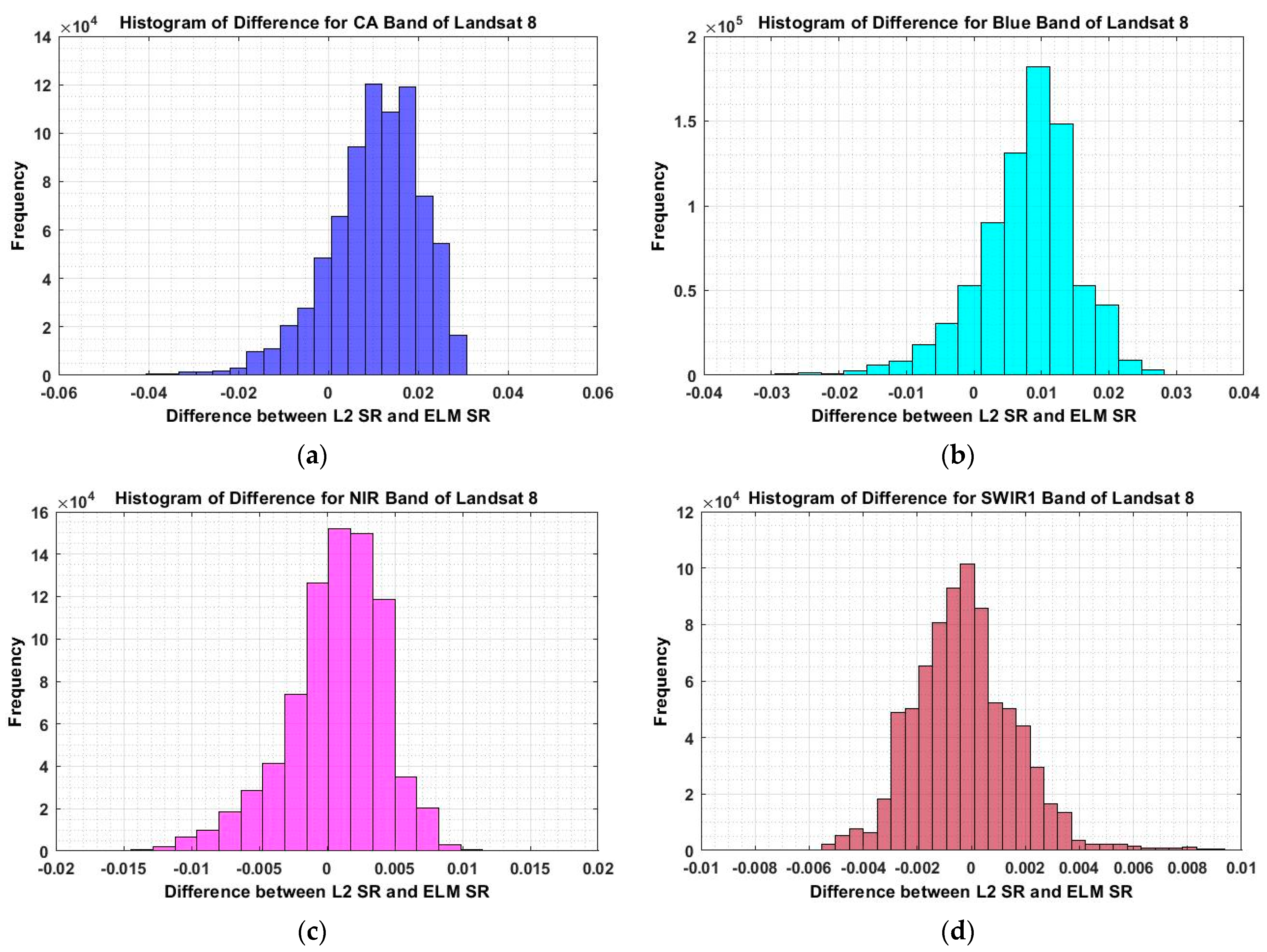
4.3.1. Landsat 8 OLI SR Validation and Evaluation Results

Figure 13 demonstrates scatter plots between Landsat 8 SR products with ELM SR for the selected ROI. Both products show good agreement with an average accuracy of 0.0104 and precision of 0.0115 across all bands of Landsat 8. The visible bands, such as coastal aerosol (CA) and blue bands, exhibited a slightly higher difference between Landsat 8 SR and ELM SR, where the data points tend to deviate from the 1:1 line in the low reflective region. In the CA and blue bands, we can see more scatteredness for low reflective regions or dark sites below 10% reflectance in the dynamic reflectance range. This might be due to the high atmospheric effect in visible wavelength bands. With a decrease in the reflectance, the part of radiation from the observed pixel decreases, and the part of background radiation (scattered in the atmosphere and created by adjacent effect) increases. In the CA and blue bands, the influence of these factors is greater, which may explain the observed effect.
Nevertheless, when we go above 10% reflectance, both products show good agreement with less scatteredness in CA and blue bands. According to Pinto et al. and Moe et al., both authors also demonstrated slight deviation from the 1:1 line in CA and blue bands while comparing Landsat 8 SR products with ground measurements [7,8]. Excluding these two bands, the other bands show a linear relationship between Landsat 8 SR product and ELM SR. The ELM validation of Landsat 8 SR products was more accurate in longer wavelength bands than in shorter wavelength bands. All the data points in the longer wavelength bands fall closer to the 1:1 line and have similar behavior with the lowest RMSE error.
Afterward, the difference between both products was calculated to check the magnitude of agreement between both products. Figure 14 shows the histogram plot of the difference between Landsat 8 SR products with ELM SR. Both products agree within ±0.01 reflectance unit in all bands except shorter wavelength bands (CA and Blue Bands). The difference in shorter wavelength bands varies within ±0.03 reflectance unit, and this might be due to the high atmospheric effect. These bands are highly affected by the aerosols and scattering components, which contributes to an increase in the path radiance observed by the sensor [49,50]. As Landsat 8 SR products were generated by the Landsat surface reflectance code (LaSRC) algorithm, this algorithm can underestimate the aerosol corrections under some conditions in CA and blue bands when aerosol optical thickness (AOT) is higher and aerosol are highly absorbing [49]. However, consistent agreement has been shown in all bands within half of reflectance unit except CA and blue bands. The reason for better agreement in the longer wavelength bands is due to less path radiance in for these bands, which minimizes the amount of correction for aerosols [49,50].
Table 2 shows the statistical metrics for validation of Landsat 8 SR over ELM SR with accuracy, precision, and RMSE. On average, the accuracy between Landsat 8 SR and ELM SR lies in the range of ~0.01 reflectance unit. This means that the Landsat 8 SR products have accuracy within 1 reflectance unit for all bands while validating with ELM SR. Similarly, the precision and RMSE results show the same (0.0019 to 0.0148) magnitude of agreements between L8 SR over ELM SR. Thus, this result indicates that the Landsat 8 SR products consistently agree with ELM SR across all the Landsat 8 OLI bands, especially on longer wavelength bands. In general, overall validation results indicate better agreement in all bands with one to half reflectance units.

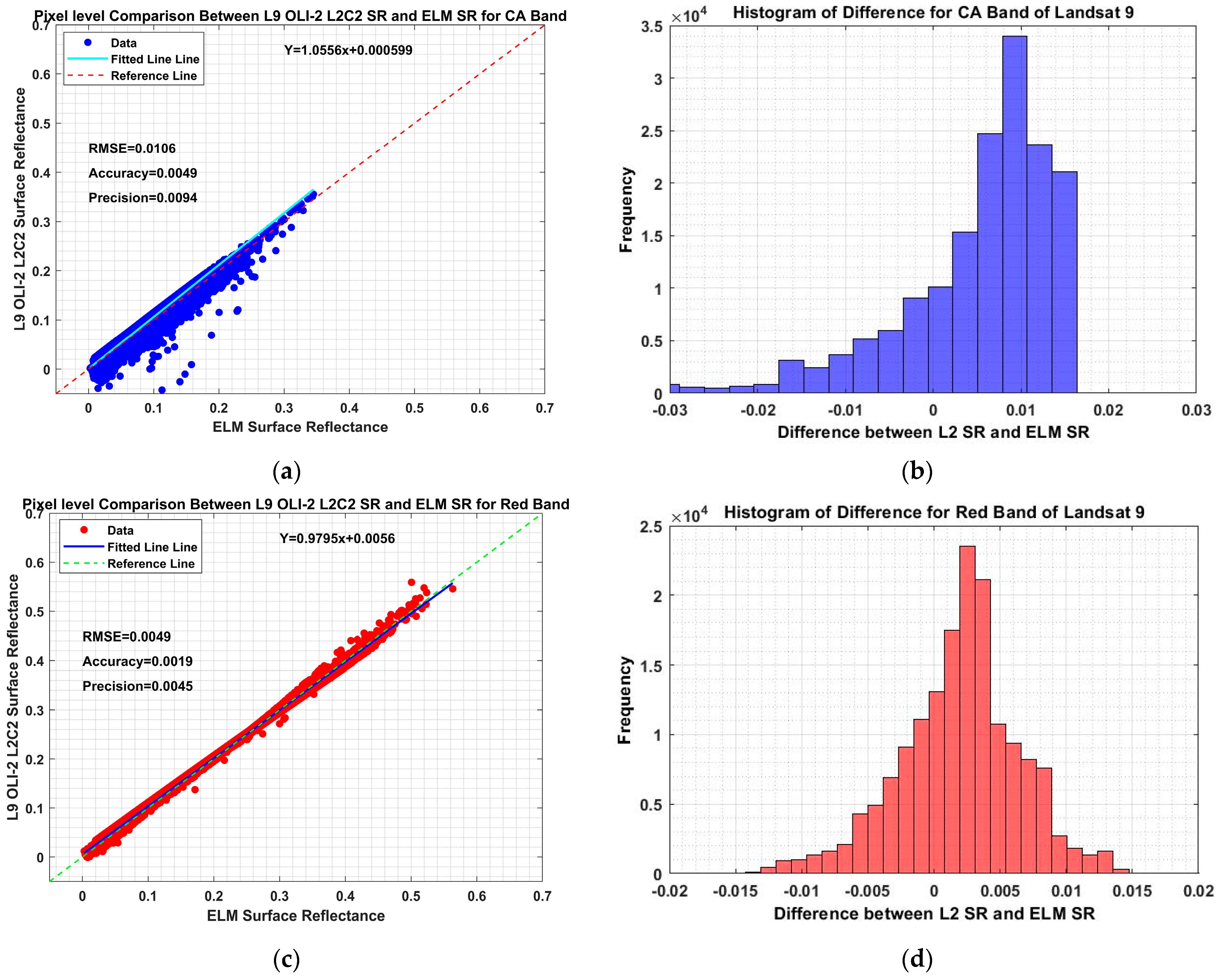
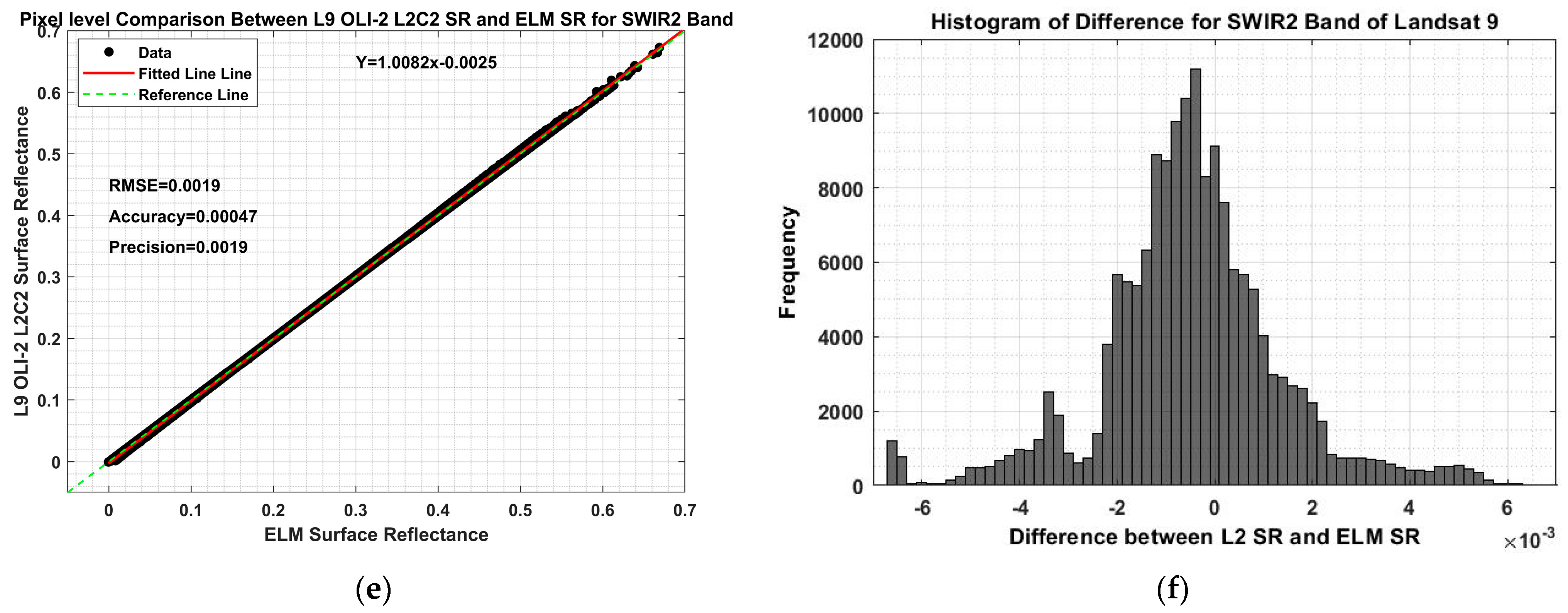
4.3.2. Landsat 9 OLI-2 SR Validation and Evaluation Results

After validating ELM SR using Landsat 8 for selected ROI, the next step was to validate Landsat 9 SR products. The absolute surface reflectance model of Algodones Dunes and Salton Sea was developed using Landsat 8 temporal trend and ground measurements from ASD and AVIRIS; the model was then adjusted for Landsat 9 spectral response. The rationale of doing this analysis was to validate Landsat 9 SR products and to check the potential of the absolute surface reflectance model to work going forth in time for predicting the ground truth reflectance. Furthermore, the SBAF was calculated and applied to adjust the spectral response of Landsat 8 with Landsat 9. As a result, the absolute surface reflectance model developed from Landsat 8 can be applied to Landsat 9 and, additionally, computed gain and bias using the ELM approach, as explained in Section 3.
Figure 15a,c,e demonstrates a pixel level scatter plot and linear relationship between Landsat 9 SR products and ELM SR. The dashed lines in each scatter plot represent a reference line for each band. Both products show good agreement with an average accuracy of 0.0049 and precision of 0.0094 across all bands of Landsat 9. In addition, in CA and blue bands, we can see the scatteredness and data points tend to deviate from the 1:1 line in the low reflective region (below reflectance of 10%). A similar deviation was observed while validating Landsat 8 SR products and ELM SR in Section 4.3.1.
Additionally, in the longer wavelength bands, both products fall closer to the 1:1 line and behave similarly, as shown in Section 4.3.1. Figure 15b,d,f shows the histogram plot of the difference between Landsat 9 SR products with ELM SR. On average, both products agree within ±0.015 reflectance unit in all bands except shorter wavelength bands (CA and blue bands).
Moreover, statistical metrics such as accuracy, precision, and RMSE between the two products were calculated, as shown in Table 3. Both products agree well within an accuracy of 0.0049 (half unit of reflectance). Precision between both products ranges from 0.0019 to 0.0094 reflectance units; this also suggests that Landsat 9 SR products are in consistent agreement with ELM SR. Additionally, RMSE also explains the same agreement between both products; the RMSE value ranges from 0.0019 to 0.01. Thus, on average, this result indicates that the Landsat 9 SR product consistently agrees with ELM SR across all the Landsat 9 OLI-2 bands, especially on longer wavelength bands.

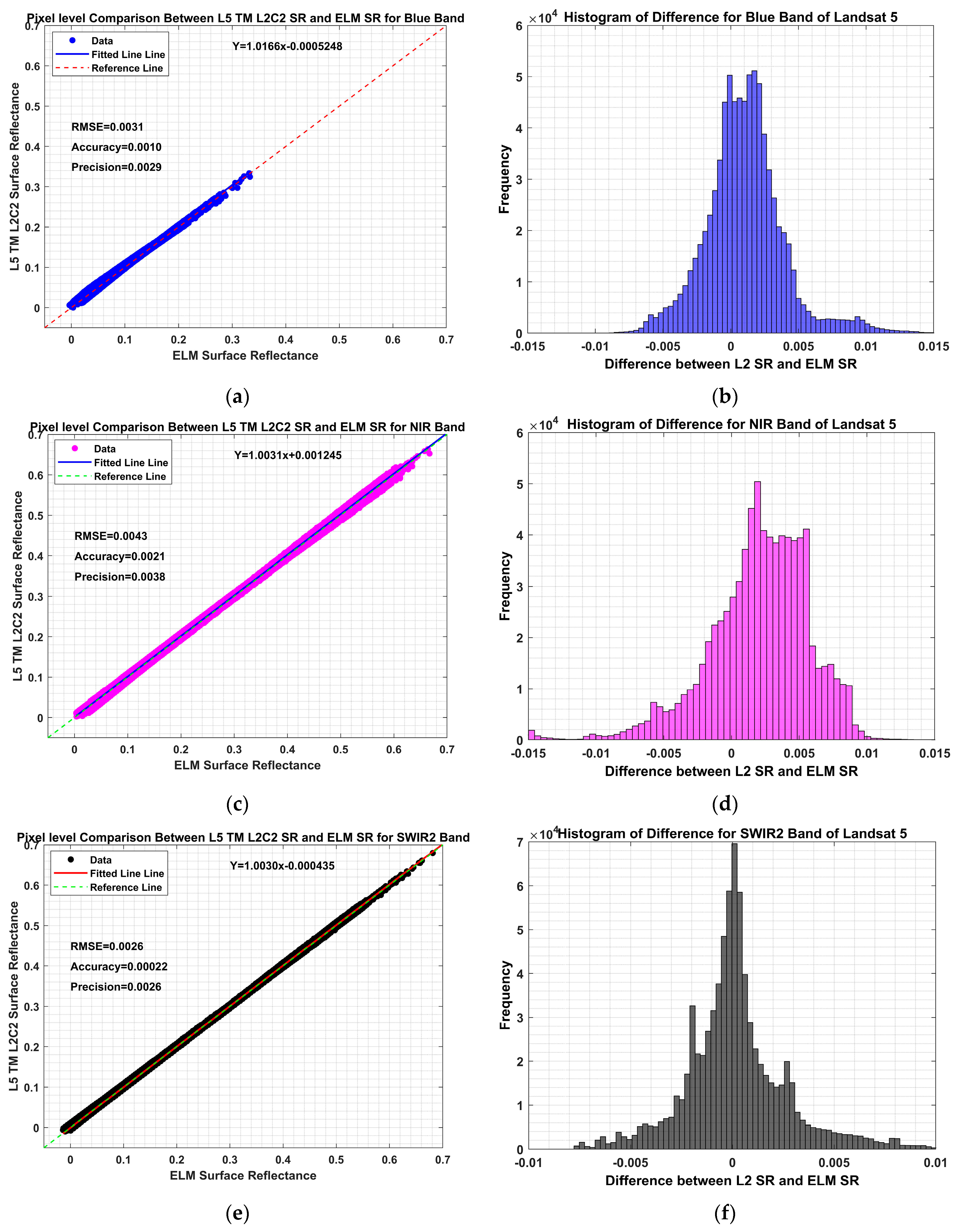
4.3.3. Landsat 5 TM SR Validation and Evaluation Results

As explained in Section 3, the absolute surface reflectance model can go back in time and predict ground truth reflectance (with the assumption that both Algodones and Salton sea is stable/predictable over the period). Therefore, it can be used for validation of any surface reflectance products using the ELM approach. To check this potential of the absolute surface reflectance model, an analysis was performed to validate Landsat 5 SR product. For that, the absolute surface reflectance model of Algodones Dunes and Salton Sea were adjusted using SBAF to match the spectral response of Landsat 5 with Landsat 8. As a result, the absolute surface reflectance model can be applied to Landsat 5 and, additionally, a computed gain and bias using the ELM approach, as explained in Section 3.
Figure 16 demonstrates a pixel level scatter plot and linear relationship between the measured value of Landsat 5 SR products and ELM SR. The dashed lines in Figure 16 represent reference lines for each bands. The analysis of six different bands of Landsat 5 SR with ELM SR products demonstrates the good quality of Landsat 5 SR products. The accuracy (0 to 0.0021) and RMSE (0.0026 to 0.0045) attest to good agreement between the two products. Figure 16 also shows a corresponding histogram plot of the difference between Landsat 5 SR products with ELM SR. On average, Landsat 5 SR products shows good agreement with an accuracy of a half unit of reflectance with ELM SR in all spectral bands. The slight deviation was usually seen in blue, which is the shorter wavelength band. The deviation in the blue band might be due to the atmospheric effect since shorter wavelength bands might be affected by aerosols components. As the wavelength continues to increase, the accuracy and precision continue to improve. Better agreement in a higher wavelength band where the atmospheric effect is minimum is observed [51]. Moreover, statistical metrics such as accuracy, precision, and RMSE between the two products were calculated, as shown in Table 4.
Furthermore, the LEDAPS algorithm for obtaining the surface reflectance for Landsat 5 has been shown under some criteria to underestimate the aerosol corrections in the blue band [51,52]. Similarly, consistent agreement was observed in all bands, which is within half a unit of reflectance unit.

4.4. Uncertainty Results

Uncertainty analysis was performed after validation of USGS SR products over ELM SR. Pixel level uncertainty was calculated for selected ROI using the Monte-Carlo Simulation method (see Section 3.2). The uncertainties associated with four input parameters were considered for the simulation, and the atmospheric coefficients (gain and bias) were calculated within their uncertainties. Monte-Carlo Simulation was performed at 160 iteration levels, giving 160 gain and bias. Furthermore, 160 simulated coefficients were applied to the image, and 160 surface reflectance images were produced for all spectral bands. Finally, the standard deviation of 160 surface reflectance images gives the overall absolute pixel level uncertainty of the ELM SR model for seven different bands of Landsat 8 sensor.
Figure 17 demonstrates absolute pixel level uncertainty images for Landsat 8 sensor (CA, green, NIR, and SWIR2 bands). In CA and green bands images, Algodones dunes and rock uncertainty range from 0.0271 to 0.0305, whereas the vegetative and water uncertainty ranges from 0.0186 to 0.0245. Similarly, in NIR and SWIR2 band images, Algodones dunes and rock uncertainty range from 0.0312 to 0.0450, whereas the vegetative and water uncertainty ranges from 0.0101 to 0.0271.
The absolute uncertainty of surface reflectance varies with the target in an image. In the visible bands such as CA, blue, and green bands, the uncertainty seems higher in dark targets such as water and vegetation and seems lower in the bright targets such as Algodones dunes and rock. While in longer wavelengths bands such as NIR, SWIR1, and SWIR2, the uncertainty seems lower in water and vegetation and seems higher in the bright target like Algodones dunes and rock. Compared to the longer wavelength bands, a slight difference was observed in shorter wavelength bands of dark targets. This is primarily due to difficulties in aerosol estimation and lower signal levels received by the OLI sensor from dark targets [49].

5. Conclusions

Due to the increased demand for SR products, a need exists to verify that L2C2 SR products are precise and accurate. Several methods for atmospherically correcting level-1 TOA reflectance and validating L2C2 SR product are carried out, although they are insufficient. This work was developed to validate SR products by developing an atmospheric correction model. At first, the ELM technique was employed in this research for atmospheric correction of remotely sensed data from at-sensor DN to ground reflectance.
The theoretical basis for ELM was carried out by selecting the sites based on the knowledge of ground truth measurements. Thus, Algodones Dunes and the Salton Sea were selected for developing the overall methodology of the project. Implementing ELM requires ground truth measurements at every point of the Landsat acquisitions for given sites. But there were limited ground truth measurements, so the absolute surface reflectance model of Algodones Dunes and Salton Sea were developed to overcome the limitation of ground truth measurements. The absolute surface reflectance of Algodones Dunes was developed using L8 SR trend, sun and sensors angle, and ground truth measurements by ASD.
Similarly, the absolute surface reflectance model of the Salton Sea was developed using L8 SR trend, sun and sensor angles, IOPs of water, and ground truth measurements by AVIRIS. The absolute surface models of Algodones dunes and Salton Sea gives ground truth measurements during Landsat acquisitions and are not limited to time constraints and have the potential to give ground truth reflectance in any time frame (going back and forth). The result of the Absolute surface reflectance model of Algodones Dunes predicts the response of Algodones Dunes and gives ground measurements over a time with an average accuracy of 0.0041 and average precision of 0.0063 overall bands of the Landsat 8 sensor. Similarly, the Salton Sea’s absolute surface reflectance model predicts the Salton Sea’s response and gives ground measurements over time with a mean absolute error (MAE) of 0.0035 overall bands of the Landsat 8 sensor. After that ELM technique applied and generates atmospheric coefficients (gain and bias) based on four inputs. These gain and bias when applied to an image produces the surface reflectance.
This study has evaluated the accuracy and reliability of level-2 surface reflectance products with surface reflectance derived from ELM. Validation of Landsat 8 OLI L2C2 SR, Landsat 9 OLI-2 L2C2 SR, and Landsat 5 TM L2C2 SR were carried out in this work. The validation of Landsat 5 TM and Landsat 9 OLI requires the SBAF correction since the absolute surface reflectance model was generated using the Landsat 8 sensor. Thus, compensating factors for matching spectral response of Landsat 5 TM and Landsat 9 OL were computed using the hyperspectral measurement taken at Algodones Dunes and Salton Sea.
When considering the surface reflectance data from ELM, the result indicates that the Landsat 8 SR products show good agreement within an average accuracy of 0.0038 reflectance unit in all bands with ELM SR for selected ROI. Precision between both products ranges from 0.0019 to 0.0113 reflectance units; this also indicates that Landsat 8 SR products show consistent agreement with ELM SR. Landsat 8 SR products are validated within ±0.01 reflectance unit in all bands except shorter wavelength bands (CA and blue bands). Data points in shorter wavelength bands tend to deviate from the 1:1 line in the low reflective region. In the CA and blue bands, we can see more scatteredness for low reflective regions or dark sites, whereas less scatteredness was observed in longer wavelength bands. However, on average, a consistent agreement was observed in all bands within half a unit of reflectance except CA and blue bands.
After validating Landsat 8 SR over ELM SR for selected ROI, the validation of Landsat 9 and 5 SR products was carried out, which requires the application of SBAF to adjust the spectral response of Landsat 8 with Landsat 9 and Landsat 5. As a result, the absolute surface reflectance model from Landsat 8 can be applied to Landsat 9 and 5. Based on the SBAF corrected model, gain and bias were calculated using ELM approach, which can be applied to Landsat 9 and Landsat 5 images to produce SR. Landsat 9 SR products agree well within an accuracy of 0.0049 (half unit of reflectance) in all bands with ELM SR. Precision between both products ranges from 0.0019 to 0.0094 reflectance units; this also means that Landsat 9 SR products show consistent agreement with ELM SR. Thus, on average, this result indicates that the Landsat 9 SR product consistently agrees with ELM SR across all the Landsat 9 OLI-2 bands, especially on longer wavelength bands. Here, in CA and blue bands, we can also see that the scatteredness and data points tend to deviate from the 1:1 line in the low reflective region (below 10% reflectance).
The Landsat 5 SR demonstrates good agreement with ELM SR products with a low accuracy value from 0 to 0.0021 and RMSE from 0.0026 to 0.0045. On average, Landsat 5 SR products agree within a half unit of reflectance with ELM SR in all spectral bands. The slight deviation was usually seen in blue, which is the shorter wavelength band. Similarly, a consistent agreement was observed in all bands. This means that TM SR and ELM SR show good agreement within a half unit of reflectance for selected ROI.
Finally, pixel level uncertainty of the ELM SR model for seven different bands of Landsat 8 sensor was done using Monte-Carlo simulation. After that, the standard deviation of 160 surface reflectance images gives the overall absolute pixel level uncertainty of the ELM SR model for seven different bands of the Landsat 8 sensor. In CA and green bands images, Algodones dunes and rock uncertainty range from 0.0271 to 0.0305, whereas the vegetative and water uncertainty ranges from 0.0186 to 0.0245. Similarly, in NIR and SWIR2 band images, Algodones dunes and rock uncertainty range from 0.0312 to 0.0450, whereas the vegetative and water uncertainty ranges from 0.0101 to 0.0271.
In conclusion, this study demonstrates the usefulness of the level-2 surface reflectance product for providing accurate information on the reflectance properties of the Earth’s surface. To guide the advantage of the developed methodology, two conclusions can be drawn: (i) The developed method is not limited to time constraints, i.e., it is independent of the temporal resolution of the sensor. The validation of the L2 SR product can be carried out in any period of satellite image acquisition. (ii) The L2 SR product can be validated in any satellite after the SBAF correction using the hyperspectral measurement.

Author Contributions

Conceptualization, M.K.C. and L.L.; methodology, M.K.C. and L.L.; formal analysis M.K.C., L.L., M.K. and C.T.P.; supervision and funding acquisition, L.L.; software M.K.C. and L.L.; Validation, M.K.C.; writing—original draft, M.K.C.; writing—review and editing; M.K.C., L.L. and C.T.P. All authors have read and agreed to the published version of the manuscript.

Funding

This project is funded by USGS EROS (Grant Number: USGS SA2000371).

Data Availability Statement

Not applicable.

Acknowledgments

The author expresses gratitude towards Larry Leigh, the Director of the Image Processing Laboratory, for providing guidance and support throughout the project development, and also thanks all the members of the lab for their unwavering support and encouragement during the project’s tenure. Additionally, the author extends a special thanks to friends Rahul and Ramita Shah, who offered their support during the project’s ups and downs. Finally, the author acknowledges the continuous support of his friend Neha Khadka and family members, who helped to reach the current position.

Conflicts of Interest

The authors declare no conflict of interest.

References

  1. Nazeer, M.; Ilori, C.O.; Bilal, M.; Nichol, J.E.; Wu, W.; Qiu, Z.; Gayene, B.K. Evaluation of atmospheric correction methods for low to high resolutions satellite remote sensing data. Atmos. Res. 2021, 249, 105308. [Google Scholar] [CrossRef]
  2. Feng, M.; Huang, C.; Channan, S.; Vermote, E.F.; Masek, J.G.; Townshend, J.R. Quality assessment of Landsat surface reflectance products using MODIS data. Comput. Geosci. 2012, 38, 9–22. [Google Scholar] [CrossRef]
  3. Wang, Y.; Liu, L.; Hu, Y.; Li, D.; Li, Z. Development and validation of the Landsat-8 surface reflectance products using a MODIS-based per-pixel atmospheric correction method. Int. J. Remote Sens. 2016, 37, 1291–1314. [Google Scholar] [CrossRef]
  4. Nazeer, M.; Nichol, J.E.; Yung, Y.-K. Evaluation of atmospheric correction models and Landsat surface reflectance product in an urban coastal environment. Int. J. Remote Sens. 2014, 35, 6271–6291. [Google Scholar] [CrossRef]
  5. Claverie, M.; Vermote, E.F.; Franch, B.; Masek, J.G. Evaluation of the Landsat-5 TM and Landsat-7 ETM+ surface reflectance products. Remote Sens. Environ. 2015, 169, 390–403. [Google Scholar] [CrossRef]
  6. Masek, J.G.; Vermote, E.F.; Saleous, N.E.; Wolfe, R.; Hall, F.G.; Huemmrich, K.F.; Gao, F.; Kutler, J.; Lim, T.-K. A Landsat surface reflectance dataset for North America, 1990–2000. IEEE Geosci. Remote Sens. Lett. 2006, 3, 68–72. [Google Scholar] [CrossRef]
  7. Badawi, M.; Helder, D.; Leigh, L.; Jing, X. Methods for earth-observing satellite surface reflectance validation. Remote Sens. 2019, 11, 1543. [Google Scholar] [CrossRef]
  8. Teixeira Pinto, C.; Jing, X.; Leigh, L. Evaluation analysis of Landsat level-1 and level-2 data products using in situ measurements. Remote Sens. 2020, 12, 2597. [Google Scholar] [CrossRef]
  9. Ben-Dor, E.; Kruse, F.; Lefkoff, A.; Banin, A. Comparison of three calibration techniques for utilization of GER 63-channel aircraft scanner data of Makhtesh Ramon, Negev, Israel. Photogramm. Eng. Remote Sens. 1994, 60, 1339–1354. [Google Scholar]
  10. Chavez, P.S. Image-based atmospheric corrections-revisited and improved. Photogramm. Eng. Remote Sens. 1996, 62, 1025–1035. [Google Scholar]
  11. Vermote, E.F.; Tanré, D.; Deuze, J.L.; Herman, M.; Morcette, J.-J. Second simulation of the satellite signal in the solar spectrum, 6S: An overview. IEEE Trans. Geosci. Remote Sens. 1997, 35, 675–686. [Google Scholar] [CrossRef]
  12. Kneizys, F.X. Users Guide to LOWTRAN 7; Air Force Geophysics Laboratory, United States Air Force: Hanscom AFB, MA, USA, 1988. [Google Scholar]
  13. Berk, A.; Bernstein, L.; Anderson, G.; Acharya, P.; Robertson, D.; Chetwynd, J.; Adler-Golden, S. MODTRAN cloud and multiple scattering upgrades with application to AVIRIS. Remote Sens. Environ. 1998, 65, 367–375. [Google Scholar] [CrossRef]
  14. Matthew, M.W.; Adler-Golden, S.M.; Berk, A.; Felde, G.; Anderson, G.P.; Gorodetzky, D.; Paswaters, S.; Shippert, M. Atmospheric correction of spectral imagery: Evaluation of the FLAASH algorithm with AVIRIS data. In Proceedings of the Applied Imagery Pattern Recognition Workshop, 2002. Proceedings, Washington, DC, USA, 16–18 October 2002; pp. 157–163. [Google Scholar]
  15. Green, R.O. Retrieval of reflectance from calibrated radiance imagery measured by the Airborne Visible/Infrared Imaging Spectrometer (AVIRIS) for lithological mapping of Clark Mountains, California. In Proceedings of the Annual JPL Airborne Visible/Infrared Imaging Spectrometer (AVIRIS) Workshop, Clark Mountains, CA, USA, 1–5 June 1990; pp. 54–90. [Google Scholar]
  16. Farrand, W.H.; Singer, R.B.; Merenyi, E. Retrieval of apparent surface reflectance from AVIRIS data: A comparison of empirical line, radiative transfer, and spectral mixture methods. Remote Sens. Environ. 1994, 47, 311–321. [Google Scholar] [CrossRef]
  17. Roberts, D.; Yamaguchi, Y.; Lyon, R. Comparison of various techniques for calibration of AIS data. NASA STI/Recon Tech. Rep. N 1986, 87, 21–30. [Google Scholar]
  18. Dwyer, J.L.; Kruse, F.A.; Lefkoff, A.B. Effects of empirical versus model-based reflectance calibration on automated analysis of imaging spectrometer data: A case study from the Drum Mountains, Utah. Photogramm. Eng. Remote Sens. 1995, 61, 1247–1254. [Google Scholar]
  19. Teillet, P.; Slater, P.; Ding, Y.; Santer, R.; Jackson, R.; Moran, M. Three methods for the absolute calibration of the NOAA AVHRR sensors in-flight. Remote Sens. Environ. 1990, 31, 105–120. [Google Scholar] [CrossRef]
  20. Ben-Dor, E.; Kindel, B.; Goetz, A. Quality assessment of several methods to recover surface reflectance using synthetic imaging spectroscopy data. Remote Sens. Environ. 2004, 90, 389–404. [Google Scholar] [CrossRef]
  21. Smith, G.M.; Milton, E.J. The use of the empirical line method to calibrate remotely sensed data to reflectance. Int. J. Remote Sens. 1999, 20, 2653–2662. [Google Scholar] [CrossRef]
  22. Perry, E.; Warner, T.; Foote, P. Comparison of atmospheric modelling versus empirical line fitting for mosaicking HYDICE imagery. Int. J. Remote Sens. 2000, 21, 799–803. [Google Scholar] [CrossRef]
  23. USGS. EarthExplorer. Available online: https://earthexplorer.usgs.gov/ (accessed on 4 August 2022).
  24. AVIRIS. Airborne Visible Infrared Imaging Spectrometer. Available online: https://aviris.jpl.nasa.gov/documents/workshop_biblios.html (accessed on 9 July 2022).
  25. Missions, S. Landsat 9 (USGS, NASA). 2022. Available online: https://www.eoportal.org/satellite-missions/landsat-9#summary (accessed on 13 March 2023).
  26. Gross, G.; Helder, D.; Begeman, C.; Leigh, L.; Kaewmanee, M.; Shah, R. Initial Cross-Calibration of Landsat 8 and Landsat 9 Using the simultaneous underfly event. Remote Sens. 2022, 14, 2418. [Google Scholar] [CrossRef]
  27. Acharya, T.D.; Yang, I. Exploring landsat 8. Int. J. IT Eng. Appl. Sci. Res. 2015, 4, 4–10. [Google Scholar]
  28. DUGUAY, C.; LEDREW, E. Estimating surface reflectance and albedo from Landsat-5 Thematic Mapper over rugged terrain. Photogramm. Eng. Remote Sens. 1992, 58, 551–558. [Google Scholar]
  29. Danner, M.; Locherer, M.; Hank, T.; Richter, K. Spectral Sampling with the ASD FIELDSPEC 4. 2015. Available online: https://gfzpublic.gfz-potsdam.de/rest/items/item_1388298/component/file_1388299/content (accessed on 13 March 2023).
  30. McCorkel, J.; Bachmann, C.M.; Coburn, C.; Gerace, A.D.; Leigh, L.; Czapla-Myers, J.S.; Helder, D.L.; Cook, B.D. Overview of the 2015 Algodones Sand Dunes field campaign to support sensor intercalibration. J. Appl. Remote Sens. 2017, 12, 012003. [Google Scholar] [CrossRef]
  31. Johnson, H.; Green, R. AVIRIS User’s Guide; JPL: Pasadena, CA, USA, 1995. Available online: https://dataverse.jpl.nasa.gov/dataset.xhtml?persistentId=hdl:2014/33639 (accessed on 13 March 2023).
  32. Kaewmanee, M. Pseudo Invariant Calibration Sites: PICS Evolution; Utah State University: Logan, UT, USA, 2018; Available online: https://digitalcommons.usu.edu/cgi/viewcontent.cgi?article=1296&context=calcon (accessed on 13 March 2023).
  33. Lee, Z.P.; Du, K.; Voss, K.J.; Zibordi, G.; Lubac, B.; Arnone, R.; Weidemann, A. An inherent-optical-property-centered approach to correct the angular effects in water-leaving radiance. Appl. Opt. 2011, 50, 3155–3167. [Google Scholar] [CrossRef] [PubMed]
  34. Pope, R.M.; Fry, E.S. Absorption spectrum (380–700 nm) of pure water. II. Integrating cavity measurements. Appl. Opt. 1997, 36, 8710–8723. [Google Scholar] [CrossRef]
  35. Chen, S.; Zhang, T. Evaluation of a QAA-based algorithm using MODIS land bands data for retrieval of IOPs in the Eastern China Seas. Opt. Express 2015, 23, 13953–13971. [Google Scholar] [CrossRef] [PubMed]
  36. Jerlov, N.; Fukuda, M. Radiance distribution in the upper layers of the sea. Tellus 1960, 12, 348–355. [Google Scholar] [CrossRef]
  37. Albert, A.; Mobley, C.D. An analytical model for subsurface irradiance and remote sensing reflectance in deep and shallow case-2 waters. Opt. Express 2003, 11, 2873–2890. [Google Scholar] [CrossRef]
  38. Roy, D.P.; Ju, J.; Kline, K.; Scaramuzza, P.L.; Kovalskyy, V.; Hansen, M.; Loveland, T.R.; Vermote, E.; Zhang, C. Web-enabled Landsat Data (WELD): Landsat ETM+ composited mosaics of the conterminous United States. Remote Sens. Environ. 2010, 114, 35–49. [Google Scholar] [CrossRef]
  39. Khakurel, P.; Leigh, L.; Kaewmanee, M.; Pinto, C.T. Extended Pseudo Invariant Calibration Site-Based Trend-to-Trend Cross-Calibration of Optical Satellite Sensors. Remote Sens. 2021, 13, 1545. [Google Scholar] [CrossRef]
  40. Chander, G.; Mishra, N.; Helder, D.L.; Aaron, D.B.; Angal, A.; Choi, T.; Xiong, X.; Doelling, D.R. Applications of spectral band adjustment factors (SBAF) for cross-calibration. IEEE Trans. Geosci. Remote Sens. 2012, 51, 1267–1281. [Google Scholar] [CrossRef]
  41. Shah, R.; Leigh, L.; Kaewmanee, M.; Pinto, C.T. Validation of Expanded Trend-to-Trend Cross-Calibration Technique and Its Application to Global Scale. Remote Sens. 2022, 14, 6216. [Google Scholar] [CrossRef]
  42. Ferrier, G.; Trahair, N. Evaluation of apparent surface reflectance estimation methodologies. Int. J. Remote Sens. 1995, 16, 2291–2297. [Google Scholar] [CrossRef]
  43. Baugh, W.; Groeneveld, D. Empirical proof of the empirical line. Int. J. Remote Sens. 2008, 29, 665–672. [Google Scholar] [CrossRef]
  44. Babu, K.; Mathur, A.; Thompson, D.R.; Green, R.O.; Patel, P.N.; Prajapati, R.; Bue, B.D.; Geier, S.; Eastwood, M.L.; Helmlinger, M.C. An empirical comparison of calibration and validation methodologies for airborne imaging spectroscopy. Curr. Sci. 2019, 116, 1101. [Google Scholar] [CrossRef]
  45. Green, R.O.; Eastwood, M.L.; Sarture, C.M.; Chrien, T.G.; Aronsson, M.; Chippendale, B.J.; Faust, J.A.; Pavri, B.E.; Chovit, C.J.; Solis, M. Imaging spectroscopy and the airborne visible/infrared imaging spectrometer (AVIRIS). Remote Sens. Environ. 1998, 65, 227–248. [Google Scholar] [CrossRef]
  46. Barsi, J.A.; Alhammoud, B.; Czapla-Myers, J.; Gascon, F.; Haque, M.O.; Kaewmanee, M.; Leigh, L.; Markham, B.L. Sentinel-2A MSI and Landsat-8 OLI radiometric cross comparison over desert sites. Eur. J. Remote Sens. 2018, 51, 822–837. [Google Scholar] [CrossRef]
  47. Helder, D.; Doelling, D.; Bhatt, R.; Choi, T.; Barsi, J. Calibrating Geosynchronous and Polar Orbiting Satellites: Sharing Best Practices. Remote Sens. 2020, 12, 2786. [Google Scholar] [CrossRef]
  48. Khadka, N.; Teixeira Pinto, C.; Leigh, L. Detection of change points in pseudo-invariant calibration sites time series using multi-sensor satellite imagery. Remote Sens. 2021, 13, 2079. [Google Scholar] [CrossRef]
  49. Doxani, G.; Vermote, E.; Roger, J.-C.; Gascon, F.; Adriaensen, S.; Frantz, D.; Hagolle, O.; Hollstein, A.; Kirches, G.; Li, F. Atmospheric correction inter-comparison exercise. Remote Sens. 2018, 10, 352. [Google Scholar] [CrossRef]
  50. Morfitt, R.; Barsi, J.; Levy, R.; Markham, B.; Micijevic, E.; Ong, L.; Scaramuzza, P.; Vanderwerff, K. Landsat-8 Operational Land Imager (OLI) radiometric performance on-orbit. Remote Sens. 2015, 7, 2208–2237. [Google Scholar] [CrossRef]
  51. Maiersperger, T.; Scaramuzza, P.; Leigh, L.; Shrestha, S.; Gallo, K.; Jenkerson, C.B.; Dwyer, J.L. Characterizing LEDAPS surface reflectance products by comparisons with AERONET, field spectrometer, and MODIS data. Remote Sens. Environ. 2013, 136, 1–13. [Google Scholar] [CrossRef]
  52. Masek, J.; Vermote, E.; Saleous, N.; Wolfe, R.; Hall, F.; Huemmrich, K.; Gao, F.; Kutler, J.; Lim, T. LEDAPS Landsat Calibration, Reflectance, Atmospheric Correction Preprocessing Code; ORNL DAAC: Oak Ridge, TN, USA, 2012. [Google Scholar]
Figure 1. Flow chart for obtaining surface reflectance using Empirical Line Method (ELM).
Remotesensing 15 02240 g001
Figure 2. Path 39 row 37/path 38 row 37 (Landsat 8 L2C2 SR image of Algodones Dunes and Salton Sea 9 October 2014).
Remotesensing 15 02240 g002
Figure 3. Temporal Plot of L2C2 SR product over Algodones Dunes by Landsat 8.
Remotesensing 15 02240 g003
Figure 4. Normalized trend of Landsat 8 BOA and TOA reflectance over Algodones Dunes.
Remotesensing 15 02240 g004
Figure 5. Normalized Temporal Plot of L2C2 SR product over Libya 4 and Algodones Dunes by Landsat 8.
Remotesensing 15 02240 g005
Figure 6. Temporal Plot of L2C2 SR product over Algodones Dunes by Landsat 7 and 8.
Remotesensing 15 02240 g006
Figure 7. Flow chart for Predicting surface reflectance over water bodies.
Remotesensing 15 02240 g007
Figure 8. Flow chart for Absolute surface reflectance model development of Algodones Dunes and Salton Sea.
Remotesensing 15 02240 g008
Figure 9. Flow chart for Estimating Uncertainty of ELM Surface Reflectance.
Remotesensing 15 02240 g009
Figure 10. Red portion represents 50 miles radius around calibrating point for evaluating SR products.
Remotesensing 15 02240 g010
Figure 11. Evaluation of absolute surface reflectance model—Algodones Dunes. (a) Landsat 8 observed reflectance (Green dot) and surface reflectance model predicted SR (Black dot); (b) Histogram of the Residual Error of the surface reflectance model (Green bar); (c) Calibrated Absolute surface reflectance model (yellow dots) for Algodones Dunes; (d) Histogram of Residual Error of the absolute surface reflectance model of Algodones Dunes and L8 observed SR (yellow bar) in the green band over Algodones Dunes.
Remotesensing 15 02240 g011
Figure 12. Evaluation of absolute surface reflectance model—Salton Sea. (a) Landsat 8 observed reflectance (Red dot) and surface reflectance model predicted SR (Black dot); (b) Histogram of Residual Error between surface reflectance model predicted SR of Salton Sea and Landsat 8 observed SR (red bar); (c) Calibrated Absolute surface reflectance model (green dots) for Salton Sea; (d) Histogram of Residual Error between calibrated absolute surface reflectance model of Salton Sea and Landsat 8 observed SR (black bar) in the red band over Salton Sea.
Remotesensing 15 02240 g012
Figure 13. (a) Pixel level scatter plot of Landsat 8 SR product and ELM SR for CA band, (b) Pixel level scatter plot of Landsat 8 SR product and ELM SR for blue band, (c) Pixel level scatter plot of Landsat 8 SR product and ELM SR for NIR band, and (d) Pixel level scatter plot of Landsat 8 SR product and ELM SR for SWIR1 band.
Remotesensing 15 02240 g013
Figure 14. (a) Histogram plot of the difference between Landsat 8 SR and ELM SR for CA band, (b) Histogram plot of the difference between Landsat 8 SR and ELM SR for blue band, (c) Histogram plot of the difference between Landsat 8 SR and ELM SR for NIR band, and (d) Histogram plot of the difference between Landsat 8 SR and ELM SR for SWIR1 band.
Remotesensing 15 02240 g014
Figure 15. (a) Pixel level scatter plot of Landsat 9 SR product and ELM SR for CA band, (b) Histogram plot of the difference between Landsat 9 SR and ELM SR for CA band, (c) Pixel level scatter plot of Landsat 9 SR product and ELM SR for red band, (d) Histogram plot of the difference between Landsat 9 SR and ELM SR for red band, (e) Pixel level scatter plot of Landsat 9 SR product and ELM SR for SWIR2 band, and (f) Histogram plot of the difference between Landsat 9 SR and ELM SR for SWIR2 band.
Remotesensing 15 02240 g015aRemotesensing 15 02240 g015b
Figure 16. (a) Pixel level scatter plot of Landsat 5 SR product and ELM SR for blue band, (b) Histogram plot of the difference between Landsat 5 SR and ELM SR for blue band, (c) Pixel level scatter plot of Landsat 5 SR product and ELM SR for NIR band, (d) Histogram plot of the difference between Landsat 5 SR and ELM SR for NIR band, (e) Pixel level scatter plot of Landsat 5 SR product and ELM SR for SWIR2 band, and (f) Histogram plot of the difference between Landsat 5 SR and ELM SR for SWIR2 band.
Remotesensing 15 02240 g016
Figure 17. (a) pixel level uncertainty image of CA band, (b) pixel level uncertainty image of green band, (c) pixel level uncertainty image of NIR band, and (d) pixel level uncertainty image of SWIR2 band.
Remotesensing 15 02240 g017
Table 1. Uncertainties associated with input parameters of ELM SR model.
Input Parameters of ModelBandsUncertaintyReferences
ASD MeasurementsCoastal Aerosol3.54%[30]
Blue3.85%
Green3.82%
Red3.99%
NIR4.22%
SWIR14.42%
SWIR24.08%
AVIRIS MeasurementsCA~SWIR28.6%[44,45]
Temporal Trend Uncertainty of Landsat 8 SensorCA~SWIR1<1%[47,48]
SWIR21.8%
Absolute Temporal Trend Uncertainty of Landsat 8 sensorCA~SWIR22%[46]
Table 2. Accuracy, Precision, and RMSE between Landsat 8 SR and ELM SR for seven bands.
BandsAccuracyPrecisionRMSE
Coastal Aerosol (443 nm)0.01040.01050.0148
Blue (482 nm)0.00780.00760.0109
Green (561.4 nm)0.00380.00360.0052
Red (654.6 nm)0.00410.00570.0070
NIR (864.7 nm)6.48 × 10⁻⁴ (~0)0.00360.0037
SWIR1 (1608.9 nm)−2.28 × 10⁻⁴ (~0)0.00190.0019
SWIR2 (2200.7 nm)2.31 × 10⁻⁴ (~0)0.00190.0019
Table 3. Accuracy, Precision, and RMSE between Landsat 9 SR and ELM SR for seven bands.
BandsAccuracyPrecisionRMSE
Coastal Aerosol (443 nm)0.00490.00940.0106
Blue (482 nm)0.00490.00750.0089
Green (561.4 nm)0.00380.00410.0056
Red (654.6 nm)0.00190.00450.0049
NIR (864.7 nm)1.56 × 10⁻⁴ (~0)0.00400.0040
SWIR1 (1608.9 nm)4.80 × 10⁻⁴ (~0)0.00240.0025
SWIR2 (2200.7 nm)−4.73 × 10⁻⁴ (~0)0.00190.0019
Table 4. Accuracy, Precision, and RMSE between L5 TM L2 SR and ELM SR for seven bands.
BandsAccuracyPrecision RMSE
Blue (482 nm)0.00100.00290.0031
Green (561.4 nm)0.00120.00260.0028
Red (654.6 nm)0.00120.00440.0045
NIR (864.7 nm)0.00210.00380.0043
SWIR1 (1608.9 nm)9.95 × 10⁻⁴ (~0)0.00300.0032
SWIR2 (2200.7 nm)2.23 × 10⁻⁴ (~0)0.00260.0026
Disclaimer/Publisher’s Note: The statements, opinions and data contained in all publications are solely those of the individual author(s) and contributor(s) and not of MDPI and/or the editor(s). MDPI and/or the editor(s) disclaim responsibility for any injury to people or property resulting from any ideas, methods, instructions or products referred to in the content.

