Coastal Aquaculture Extraction Using GF-3 Fully Polarimetric SAR Imagery: A Framework Integrating UNet++ with Marker-Controlled Watershed Segmentation

Abstract

Coastal aquaculture monitoring is vital for sustainable offshore aquaculture management. However, the dense distribution and various sizes of aquacultures make it challenging to accurately extract the boundaries of aquaculture ponds. In this study, we develop a novel combined framework that integrates UNet++ with a marker-controlled watershed segmentation strategy to facilitate aquaculture boundary extraction from fully polarimetric GaoFen-3 SAR imagery. First, four polarimetric decomposition algorithms were applied to extract 13 polarimetric scattering features. Together with the nine other polarisation and texture features, a total of 22 polarimetric features were then extracted, among which four were optimised according to the separability index. Subsequently, to reduce the “adhesion” phenomenon and separate adjacent and even adhering ponds into individual aquaculture units, two UNet++ subnetworks were utilised to construct the marker and foreground functions, the results of which were then used in the marker-controlled watershed algorithm to obtain refined aquaculture results. A multiclass segmentation strategy that divides the intermediate markers into three categories (aquaculture, background and dikes) was applied to the marker function. In addition, a boundary patch refinement postprocessing strategy was applied to the two subnetworks to extract and repair the complex/error-prone boundaries of the aquaculture ponds, followed by a morphological operation that was conducted for label augmentation. An experimental investigation performed to extract individual aquacultures in the Yancheng Coastal Wetlands indicated that the crucial features for aquacultures are Shannon entropy (SE), the intensity component of SE (SE_I) and the corresponding mean texture features (Mean_SE and Mean_SE_I). When the optimal features were introduced, our proposed method performed better than standard UNet++ in aquaculture extraction, achieving improvements of 1.8%, 3.2%, 21.7% and 12.1% in F1, IoU, MR and insF1, respectively. The experimental results indicate that the proposed method can handle the adhesion of both adjacent objects and unclear boundaries effectively and capture clear and refined aquaculture boundaries.

1. Introduction

Coastal aquaculture has become one of the main sources of animal protein and plays an important role in supplying food and supporting nutrition and security around the world. According to the Food and Agriculture Organization of the United Nations, aquaculture is one of the fastest-growing food providers, producing up to 114.5 million tons in total [1]. China is the world’s largest aquaculture country (with 8.346 million hectares), and the cumulative exports have reached 51.42 million tons, accounting for 60% of the worldwide total. Although the prosperous development of aquaculture has led to tremendous economic benefits, it has also had negative impacts on the local coastal environment and regional sustainable development. Moreover, most of the reported fishery statistics and studies only focus on the area of each aquaculture region, ignoring the detailed spatial location and distribution of aquaculture water resources. Therefore, accurately mapping the spatial distribution and detailed boundary information of aquacultures is crucial for sustainable management and the detection of illegal aquacultures and can further provide important support for policy development and implementation at regional, national and global levels. Satellite remote sensing technology has the advantages of a wide view with a large coverage area and short revisit period, thus providing important support for mapping the spatial distribution of aquacultures at large scales [2,3]. Current studies on aquaculture mapping mainly use optical remote sensing data [4,5]. For example, Chinese offshore raft and cage aquaculture areas (in 2018) were investigated using an unsupervised classification algorithm and artificial interpreters based on Landsat 8 remote sensing images, with an extraction accuracy of 87.35% [6], and a hierarchical cascade convolutional neural network was used for the finer resolution mapping of marine aquacultures, which also achieved a good performance on Worldview-2 imagery [7]. In addition, biophysical parameters obtained from Sentinel-2 time series images were utilised to accurately map and analyse the spatial pattern and distribution of aquaculture ponds in China in 2019 [8], and a workflow for automatic fishpond mapping was implemented on the Google Earth Engine (GEE) platform using Sentinel-2 images [9]. Meanwhile, a highly efficient method for mapping aquaculture ponds using Landsat 8 images based on the GEE platform was proposed to extract the aquaculture pond regions in the Chinese coastal zone in 2017 [10]. Moreover, the spatiotemporal dynamics of aquaculture pond areas in China over the past few decades were analysed using a time series of Landsat images [4,5,11]. However, optical satellite data are easily affected by cloudy/rainy weather since it limits data availability and quality, particularly in coastal areas with high humidity [12]. Compared with optical sensors, satellite synthetic aperture radar (SAR) systems have the capability of all-weather acquisition and strong penetration and, therefore, have become a promising data source for coastal aquaculture monitoring in recent years [13]. The existing methods of aquaculture extraction based on SAR images can be divided into two modes: single polarisation and full polarisation. The former mode mainly utilises the backscatter intensities of single-polarisation or dual-polarisation signals, with limited polarisation features [14]. In contrast, fully polarimetric SAR data contain four polarimetric channels, which can provide richer scattering information than that in the single polarisation mode [15]. Moreover, polarimetric decomposition can be used to obtain important polarisation features that reveal the scattering mechanism for different ground objects [16,17]. Wan et al. applied polarimetric decomposition to fully polarised SAR data for water body extraction in complex coastal areas and obtained an accuracy of 94.74%, thus effectively compensating for the lack of a reliable single-polarisation method [18].

Gaofen-3 (GF-3), as the first fully polarimetric C-band SAR satellite of China, was launched on 10 August 2016 and provides data at a metre-level resolution. Consequently, many datasets are now available for the precise monitoring of aquacultures. Several studies have used GF-3 for aquaculture monitoring but have mainly focused on marine floating raft aquacultures [19,20]. In contrast, there have been few studies that use GF-3 for the identification of inland aquaculture ponds, which are permanently water-filled surfaces surrounded by embankment dikes and generally have rectangular shapes [21]. They are typically independent closed shallow water bodies with an average depth of less than 2 m [22]. In SAR images, smooth aquaculture surfaces have a lower backscatter signal than rougher non-water surfaces because it corresponds to specular reflection. Previous studies have mainly focused on extracting large-scale aquaculture information from medium- and low-resolution remote sensing images. The dikes around many aquaculture ponds are narrow, usually only a few metres wide, making it difficult to distinguish adjacent aquacultures due to the limitation of the low spatial resolution of the images. Although open-access time series Sentinel-1 data have been introduced for the large-scale mapping of intensive aquaculture ponds, the detailed features of small ponds with complex water information may be difficult to identify, and adjacent dikes may be difficult to distinguish [3,12,13,14]. GF-3 outperforms Sentinel-1 in terms of spatial resolution and polarised scattering information, making it a superior choice for aquaculture monitoring and analysis. The higher spatial resolution of GF-3 images enables the details of the aquacultures and the surrounding dikes to be captured, especially for small-scale aquaculture ponds. Furthermore, fully polarised GF-3 images contain rich polarised scattering information, providing a comprehensive and detailed view of the aquaculture areas. To improve the accuracy of aquaculture extraction, researchers introduced simple watershed thresholding and machine learning algorithms (decision trees, support vector machines, random forests, etc.) into aquaculture recognition and effectively improved the aquaculture extraction accuracy. However, when using these traditional shallow learning methods, the boundaries of the extracted ponds are often unclear, and the ponds are easily confused with other ground objects, especially in small-scale pond areas with complex water information.

Deep learning can be used to learn high-level context features and provides powerful data mining and feature extraction capabilities; therefore, it has received extensive attention in the remote sensing field. In recent years, convolutional neural network (CNN) and fully convolutional network (FCN) models have been rapidly developed and are widely used in remote sensing image feature classification, target detection and semantic segmentation tasks. Fu et al. used an automatic labelling method based on a CNN to extract marine aquaculture areas and achieved significant improvements in visual and quantitative performance [7]. Cui et al. used an FCN to automatically extract floating raft aquaculture areas from Gaofen-1 images [23]. Zeng et al. proposed an FCN combined with an RCSA mechanism for the semantic segmentation of aquaculture ponds. Experiments based on high-spatial-resolution optical satellite images show that the overall accuracy of the proposed method was significantly better than that of other methods [24]. An FCN is an end-to-end deep supervisory network architecture that expands the perceptual domain by convolutional layer downsampling, maximises the use of context information and improves classification accuracy [25]; therefore, FCNs are being increasingly employed in studies of high-resolution optical images and fully polarised SAR images to extract a single category of ground objects. FCN-based UNet, as an updated convolutional network, was recently introduced in biomedical image segmentation. Compared with an FCN, UNet consists of a contracting path to capture contextual information and a symmetric expanding pathway that enables precise localisation, and it works well in cases with small training datasets and yields precise segmentation results [26]; for example, a semantic segmentation neural network was combined with UNet with deep residual learning for road area extraction from high-resolution remote sensing images [27]. Furthermore, a multiscale attention UNet model with dilated convolution and offset convolution (MDOAU-net) was introduced in SAR image segmentation for aquaculture raft monitoring [28]. Subsequently (2018–2020), as an updated strategy, UNet++, a deeply supervised encoder–decoder network, was introduced with redesigned skip pathways/connections and efficient ensembles of UNets of different depths. UNet++ has displayed a strong performance in alleviating issues related to the unknown depth of optimal architectures and the semantic gap between the feature maps of the encoder and decoder subnetworks, thus supporting more accurate segmentation tasks as a highly flexible feature fusion scheme [29,30].

The marker-controlled watershed (MCW) method is an intuitive and fast segmentation approach that can be used to split bordering objects and limit the oversegmentation problem in medical image processing [31,32,33,34]. The watershed algorithm is optimised by combining prior knowledge to obtain a reliable segmentation effect [33,35]. Additionally, numerous deep learning models have been proposed for medical images and have achieved an outstanding performance [36,37]. To address the challenge of overlapping and to divide touching nuclei into several individual nuclei, Xie et al. presented an efficient computing framework by integrating deep CNNs with MCW. The experimental results indicated that the proposed method achieved substantial improvements compared with other state-of-the-art methods [38]. Other studies have combined MCW with a deep learning model to enhance the segmentation efficiency and improve accuracy [39,40,41].

The extraction of coastal aquaculture ponds is similar to the segmentation of nuclei cells in medical images. Both aquaculture ponds and the nuclei cells are concentrated and densely distributed, with distinct spatial geometrical features, where the ponds are regular rectangles and the cells are round or elliptical. When segmenting aquaculture ponds, the following problems that exist in cell segmentation often occur: adhesion of adjacent objects, unclear boundaries and objects that are easily confused with the background. As a result, it is difficult to distinguish the dikes of small-scale aquaculture ponds from the water bodies inside the ponds due to the constraints of satellite image resolution. Considering that the fish breeds, methods and types of aquaculture are being gradually diversified, which has increased the difficulty of aquaculture management, accurately mapping aquaculture areas is important for their sustainable management and for policy-makers. In this study, we chose the Gaofen-3 Polarimetric SAR Imagery dataset and explored a novel model that integrates two UNet++ subnetworks with the marker-controlled watershed (MCW) segmentation strategy, where boundary patch refinement (BPR) postprocessing was employed, to obtain refined maps of the coastal aquacultures in Yancheng, China.

2. Study Area and Data

2.1. Study Area

This study focused on a typical aquaculture area in the Yancheng Coastal Wetlands Nature Reserve, which is located on the eastern coast of the Jiangsu Province (32°52′~33°6′N, 120°45′~120°56′E), China, as shown in Figure 1. The study area is characterised by a subtropical monsoon climate, sufficient rain, abundant tidal flats and shallow bays. The superior natural conditions provide suitable conditions for the large-scale construction of aquaculture ponds. Fish, shrimp and crab are the main types of aquaculture species in the study area. The ponds are densely distributed and most of them have a regular rectangular shape and are separated by relatively narrow dikes, embankments or levees.

2.2. Satellite Data and Data Processing

Gaofen-3 (GF-3) was the first civilian C-band full polarimetric SAR satellite in China and was launched by the China National Space Administration (CNSA) in August 2016. GF-3 carries 12 different imaging modes aboard, ranging from single-polarisation (HH or VV) to dual-polarisation (HH + HV or VH + VV) and quad-polarisation (HH + HV + VH + VV), with a resolution of 1 to 500 m [42]. The GF-3 satellite has the ability to monitor ocean, land and coastal areas under any weather condition and effectively compensates for optical image defects and susceptibility to cloudy and rainy weather, ocean tides and air humidity [43]. Such characteristics render GF-3 suitable for aquaculture monitoring in coastal areas.

In this study, we used C-band fully polarimetric GF-3 images (http://sasclouds.com/chinese/home/, accessed on 15 March 2021) with a resolution of 4.5 m × 5 m in the azimuth and range directions, acquired on 12 October 2017 in the Quad-Polarisation Stripmap 1 (QPS1) imaging mode. The data were preprocessed with the PolSARpro software, which included multilooking processing and a refined Lee filter that was used to reduce speckle and enhance edges and other features.

3. Methodology

An overview of the proposed method is illustrated in Figure 2. The proposed method combines three prominent steps: (I) polarimetric feature extraction and optimisation, (II) segmentation combining UNet++ and MCW segmentation and (III) accuracy assessment. First, the polarimetric segmentation algorithm was applied to fully polarimetric GaoFen-3 SAR imagery to extract the polarimetric scattering features, four of which were optimised according to the separability index. Second, we proposed an aquaculture extraction framework that integrates UNet++ with an MCW segmentation strategy, where a boundary patch refinement (BPR) postprocessing strategy was employed for coastal aquaculture extraction. Finally, the accuracy of the experimental results was evaluated to verify the feasibility of the method.

3.1. Extraction and Optimisation of GF-3 Fully Polarimetric Scattering Features

GF-3 full-polarisation SAR data contain valuable polarimetric scattering information, which corresponds to the physical scattering mechanism of ground objects and can effectively reflect their composition and structure information. Polarimetric decomposition is often applied to extract the scattering information in polarimetric SAR data applications [44]. In this research, 13 polarimetric scattering features were extracted by using four polarisation decomposition algorithms: H/A/Alpha decomposition, Freeman3 decomposition, Huynen decomposition and Yamaguchi4 decomposition. In addition, 6 other polarisation features and 3 backscattering coefficients were obtained, for a total of 22 polarimetric features, as shown in

Table 1. Descriptions of the 22 polarimetric scattering features used in the study.

Polarimetric Decompositions Methods	Acronyms of Features	Physical Meanings
H/A/Alpha	Entropy	Polarimetric entropy
	Anisotropy	Polarimetric anisotropy
	Alpha	Average polarisation scattering angle
Freeman3	Freeman_Odd	Surface scattering
	Freeman_Dbl	Double-bounce scattering
	Freeman_Vol	Surface scattering
Huynen	Huynen_T11	Symmetry factor
	Huynen_T22	Asymmetric factor
	Huynen_T33	Irregularity factor
Yamaguchi4	Yamaguchi4_Odd	Surface scattering
	Yamaguchi4_Dbl	Double-bounce scattering
	Yamaguchi4_Vol	Surface scattering
	Yamaguchi4_Hlx	Helix scattering
Other polarisation features	SE	Shannon Entropy
	SE_I	Intensity component of SE
	SE_P	Polarisation component of SE
	Serd	Single-bounce eigenvalue relative difference
	Derd	Double-bounce eigenvalue relative difference
	RVI	Radar Vegetation Index
Backscattering coefficients	HH	Co-polarised horizontal scattering matrix elements
	HV	Cross-polar scattering matrix elements
	VV	Co-polarised vertical scattering matrix elements

.

To a certain extent, combining multiple features can mitigate the phenomena of low discrimination and easy confusion among ground objects, but considering too many features can easily lead to feature redundancy and even cause a “dimension disaster”. The selection of suitable features is critical for classification. Therefore, to select the useful features for separating aquacultures from dikes and other nonaquaculture land cover classes, the separability index (SI) was calculated for all polarimetric features [45,46,47]. The SI is defined as:

$$S{I}_{a,b}=\frac{\left|{\mu }_a-{\mu }_b\right|}{S_a+S_b}$$

(1)

where $\mu$ and $S$ are the mean values and standard deviations of classes $a$ and $b$ for a particular feature. The higher the value of $S{I}_{a,b}$, the better the separability between class $a$ and class $b$ [48]. In particular, an $S{I}_{a,b}$ value between 0.8 and 1.5 indicates an authentic feature and $S{I}_{a,b}$ values greater than 2 indicate that a feature is nearly completely separated from inclusion of other classes [49].

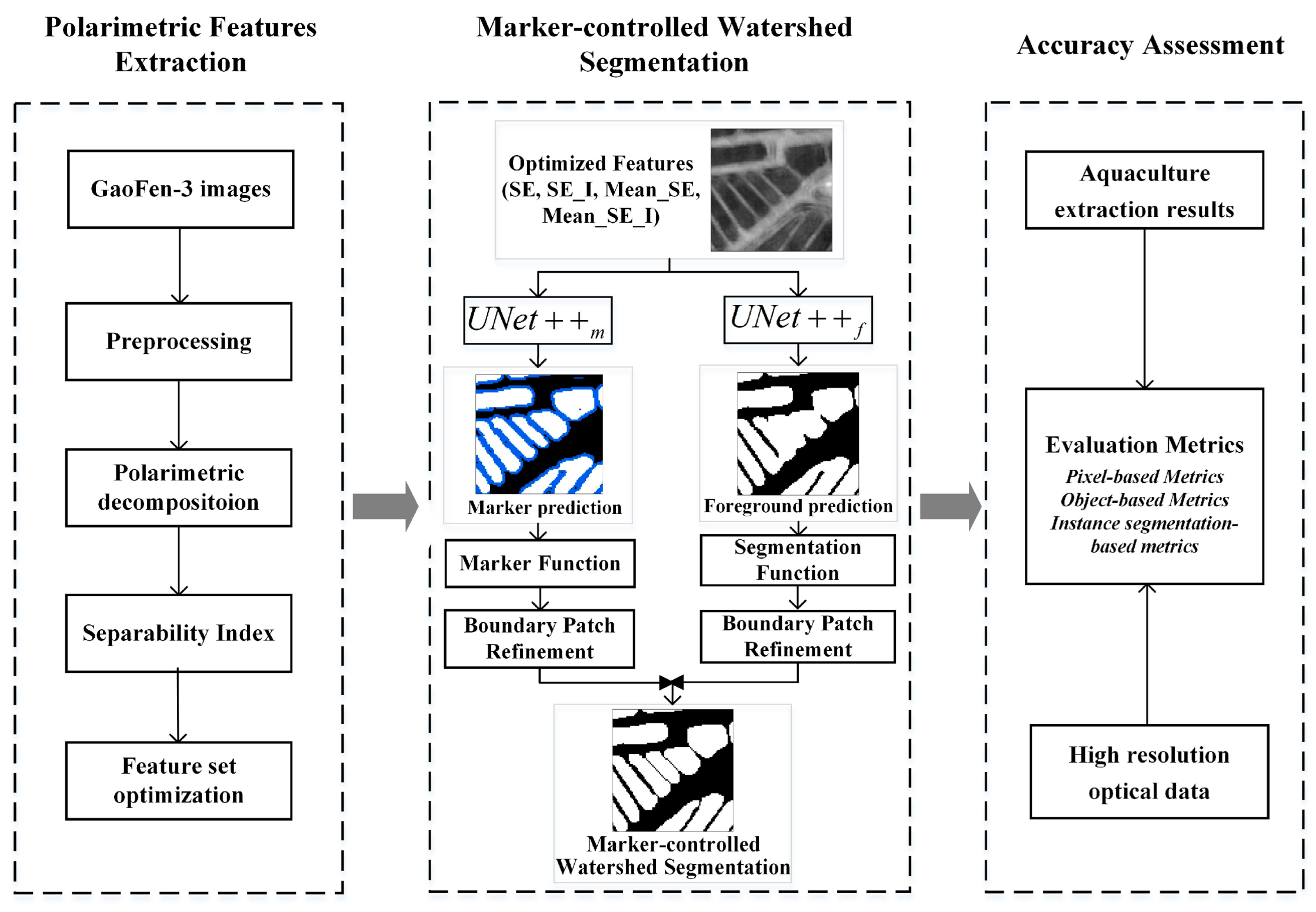
3.2. Segmentation Using Combined UNet++ and the Marker-Controlled Watershed Strategy

The proposed segmentation framework combines three prominent image processing techniques: UNet++, MCW segmentation and a boundary patch refinement strategy. In this study, two UNet++ networks are trained: the first network UNet++_m predicts the markers of coastal aquacultures, and the second network UNet++_f predicts the image foreground (coastal aquacultures). The two UNet++ subnetworks are then transformed into a marker function and a segmentation function with a mathematical morphology pipeline. MCW segmentation is used to obtain the final segmentation results based on the generated markers and foreground. As a postprocessing mechanism, the boundary patch refinement strategy is applied to refine the marker and foreground prediction results.

3.2.1. UNet++ Architecture

UNet is an end-to-end encoder–decoder-based architecture that consists of a contracting path to capture contextual information and a symmetric expanding pathway that enables precise localisation [26]. The overall architecture of UNet++ is shown in Figure 3 and mainly consists of convolution units, downsampling and upsampling modules, and skip connections between convolution units [50]. UNet++ is constructed from UNet (the blue components in Figure 3) by adding dense skip connections (shown in black) to enable dense feature propagation along skip connections.

Let $x^{i,j}$ denote the output of $X^{i,j}$, where $i$ is the index of the downsampling layer along the encoder and $j$ is the index of the convolution layer of the dense block along a skip pathway. The stack of feature maps represented by $x^{i,j}$ is computed as

$$x^{i,j}=\{\begin{array}{c}\mathscr{H}\left(\mathcal{D}\left(x^{i-1,j}\right)\right),\hspace{1em}\hspace{1em}\hspace{1em}\hspace{1em}\hspace{1em} j=0\\ \mathscr{H}\left(\left[{\left[x^{i,k}\right]}_{k=0}^{j-1},\mathcal{U}\left(x^{i+1,j-1}\right)\right]\right),j>0\end{array}$$

(2)

where function $\mathscr{H}(\cdot )$ is a convolution operation followed by an activation function, $\mathcal{D}(\cdot )$ and $\mathcal{U}(\cdot )$ denote a downsampling layer and an upsampling layer, respectively, and $[ ]$ denotes the concatenation layer. Nodes at level $j=0$ receive only one input from the previous layer of the encoder; nodes at level $j=1$ receive two inputs, both from the encoder subnetwork but at two consecutive levels; and nodes at level $j>1$ receive $j+1$ inputs, of which $j$ inputs are the outputs of the previous $j$ nodes of the same skip connection and the $j+1^{th}$ input is the upsampled output from the lower skip connection. The reason that all prior feature maps accumulate and arrive at the current node is that a dense convolution block is applied along each skip connection.

When $i=0, x^{i-1,0}$ in Equation (2) becomes $x^{-1,0}$, which serves as the input of the network. The images at node $x^{0,4}$ are processed through (1,1) convolution to integrate the multichannel images back into single-channel images as the network output. In our study, the nodes $x^{0,0}$, $x^{1,0}$, $x^{2,0}$, $x^{3,0}$ and $x^{4,0}$ represent images of size 256 × 256, 128 × 128, 64 × 64, 32 × 32 and 16 × 16, respectively, with 64, 128, 256, 512 and 1024 channels, respectively. Notably, the deep supervision mechanism in the initial UNet++ network is not used. MSE loss is only measured for $x^{0,4}$ during the model training stage and only $x^{0,4}$ is used as the network output for further assessment.

As shown in Figure 2, the proposed method consists of two parallel UNet++ networks, where UNet++_m is for marker prediction and UNet++_f is devoted to foreground prediction. Detailed information on the two subnetworks is illustrated below.

3.2.2. Marker and Foreground Predictions

In aquaculture areas with a dense spatial distribution, the inhomogeneity of the brightness, pattern of the connecting boundaries and data imbalance problem caused by the small total number of pixels at the adjacent boundary compared with the number in the whole area make the segmentation of adjacent aquacultures challenging. UNet++_m is designed for marker prediction, which indicates the locations of aquacultures. The marker function predicts the probability that each pixel represents a marker and defines the segmentation seeds for MCW segmentation. It is very important to extract the markers that truly represent the true objects. Traditional segmentation generally divides an image into two classes: foreground and background. Here, to extract the markers efficiently and distinguish aquacultures from the surrounding dikes, we divide images into three categories in the marker prediction process: foreground, background and dikes. First, a UNet++ network is applied to obtain a binary segmentation map containing two classes (background and aquaculture). Second, label augmentation based on morphological operations is performed based on the segmentation map to create a third class corresponding to the areas between aquacultures (dikes). We use a 3 × 3 square structuring element for $S_e$. The new class contains a slightly thicker region than the original gap between aquacultures. In this case, the image is divided into three types: foreground, background and dikes. Among them, the pixels corresponding to the foreground tend to have a higher probability of being aquaculture and are considered marker results of the UNet++_m network, which are further used to define segmentation seeds in subsequent MCW segmentation.

Comparatively, the UNet++_f network used for foreground prediction is relatively simple. It roughly divides an image into two categories: aquaculture and nonaquaculture areas. The aquaculture class result is considered the foreground. Then, the results of marker prediction and foreground prediction are used as the inputs for MCW segmentation.

3.2.3. Marker-Controlled Watershed Segmentation

Traditionally, watersheds are used in hydrological simulations, and oversegmentation problems are common [31]. MCW segmentation can better address oversegmentation and optimise watershed algorithms by considering the prior knowledge [33,35]. It is a nonparameter transformation method, and a marker function and a segmentation function are used to generate individual fields, with the ability to alleviate the boundary adhesion phenomenon [34,51]. During the process, the foreground markers obtained from marker prediction are regarded as segmentation seeds, and the background parts obtained during segmentation prediction are regarded as topological surfaces. Although a single deep learning model may display good extraction performance for aquacultures with large areas, the effectiveness is limited in aggregated areas of small-sized, tightly packed ponds [52,53]. Combinatorial approaches that integrate MCW and CNN have proven effective in segmenting touching and overlapping nuclei that are densely clustered in medical images [38,39]. In this study, we combine the MCW framework with two UNet++ subnetworks to address the adhesion and overlapping problems between adjacent ponds. As illustrated above, UNet++_m is used to calculate the probability that each pixel represents a marker and split the connected components corresponding to aquaculture markers. Then, UNet++_f can predict the image foreground, which is then transformed into a segmentation function using mathematical morphology operators. Finally, we use the MCW algorithm to obtain the final segmented and separated aquaculture result according to the marker function and segmentation function.

3.2.4. Boundary Patch Refinement

As a postprocessing mechanism, the boundary patch refinement (BPR) framework can be applied to improve the boundary quality in instance segmentation [54]. In this study, we add a BPR framework to augment both the UNet++_m and UNet++_f networks. An overview of the boundary patch refinement framework is shown in Figure 4. First, a sliding-window algorithm is implemented along the edges of the segmentation result to extract a series of patches with complex and error-prone boundaries. Specifically, we design a 7 × 7 operator with values all equal to 1 to extract the binary map of the coarse segmentation result. The step size of the sliding window is set to 2, and the V value of the corresponding patch is calculated. When the value of V is greater than 10, the patch is regarded as an error-prone boundary, as shown in Figure 4b. However, coarse extraction results are often redundant, and Euclidean distances are then used here to filter and remove a subset of patches and obtain sparse patch results, as shown in Figure 4c. In general, the larger the overlap, the better the segmentation performance, but the computational cost is high. The threshold of the Euclidean distance can be adjusted to control the degree of overlap to achieve a better balance of speed and accuracy. Moreover, sample slices (boundary patches) in the original images that have the same position as the filtered sparse patches are extracted. Then, the concatenated original image sample slices (Figure 4e) and the corresponding sample patches (Figure 4f) are again trained in a new UNet++ network to obtain the refined slice boundary results (as shown in Figure 4g), which are used to replace the coarse segmentation results at the corresponding positions to obtain the final fusion results.

In this study, we combine UNet++ with MCW segmentation and introduce the boundary patch refinement (BPR) postprocessing method to propose a novel framework for coastal aquaculture extraction, called MCW (3^BPR, 2^BPR), where 3 represents the three categories in the marker prediction (foreground, background and dikes), 2 represents the two categories in the foreground prediction (aquaculture and nonaquaculture) 3^BPR and 2^BPR indicate that BPR postprocessing is applied in the UNet++_m and UNet++_f subnetworks, respectively.

3.3. Accuracy Assessment and Comparison

To verify the effectiveness of the proposed method, five comparative experiments are performed in this study with two machine learning models (support vector machine (SVM) and random forest (RF)) and three deep learning methods (UNet, LinkNet and UNet++). The aquaculture extraction accuracy is quantitatively evaluated with four accuracy metrics: F1 score, mean intersection over union (IoU), matching rate (MR) and instantiated F1 score (insF1). F1 and IoU are pixel-based metrics, presenting the overall classification accuracy of the results, and are calculated based on a statistical analysis of the classified pixels to evaluate the accuracy of semantic segmentation [40]. The calculations are as follows:

$$precision=\frac{TP}{TP+FP}$$

(3)

$$recall=\frac{TP}{TP+FP}$$

(4)

$$F1=2\times \frac{precision\times recall}{precision+recall}$$

(5)

$$IoU=\frac{TP}{TP+FP+FN}$$

(6)

where TP, FP, TN and FN denote true positive, false positive, true negative and false negative, respectively.

Aquaculture ponds are structures with relatively regular textures, most of which are approximately rectangular, similar to buildings. The matching rate (MR) is an object-based evaluation metric designed to consider the geometrical properties of building extraction results [55], and it is introduced here to evaluate the geometric quality of aquaculture segmentation results. MR represents the numeric ratio between the number of matched objects and the total number of objects and is defined as follows:

$$E_{os}\left(O_i,S_j\right)=1-\frac{\left|S_j\cap O_i\right|}{\left|O_i\right|}$$

(7)

$$E_{us}\left(O_i,S_j\right)=1-\frac{\left|S_j\cap O_i\right|}{\left|S_j\right|}$$

(8)

$$M\left(O_i,S_j\right)=\{\begin{array}{c}0,E_{os}\left(O_i,S_j\right)>T\left|\right|E_{us}\left(O_i,S_j\right)>T\\ 1,E_{os}\left(O_i,S_j\right)\le T\&E_{us}\left(O_i,S_j\right)\le T\end{array}$$

(9)

$$MR=\frac{{\displaystyle \sum {}_{i,j}M(O_i,S_j)}}{N_{O_i}}$$

(10)

where $O_i$ is a reference object in a ground-truth map L, $S_j$ is a segmented object in the prediction map P, $E_{os}$ and $E_{us}$ represent the oversegmentation error and undersegmentation error, respectively, and $M\left(O_i,S_j\right)$ is the matching rate for $O_i$ and $S_j$.

In addition, InsF1 is applied in this study to further evaluate the instance segmentation ability of the network model. InsF1 is based on the IoU and was used in the Urban 3D challenge in 2018 and the Ali Tianchi Building Intelligence Census Competition in 2020 as a criterion for assessing instance segmentation performance [56]. InsF1 is instantiated based on TP, FP and FN results under the constraint that the IoU is greater than 0.5. The equations are as follows:

$$precisio{n}_{IoU>0.5}=\frac{T{P}_{IoU>0.5}}{T{P}_{IoU>0.5}+F{P}_{IoU>0.5}}$$

(11)

$$recal{l}_{IoU>0.5}=\frac{T{P}_{{}_{IoU>0.5}}}{T{P}_{{}_{IoU>0.5}}+F{N}_{{}_{IoU>0.5}}}$$

(12)

$$InsF1=\frac{precisio{n}_{IoU>0.5}\times recal{l}_{IoU>0.5}}{precisio{n}_{IoU>0.5}+recal{l}_{IoU>0.5}}$$

(13)

4. Experiments and Results

4.1. Experimental Setup

All the algorithms are implemented based on PyTorch, and the experiments are conducted on an NVIDIA RTX3080 with 10 GB of memory. For the coarse segmentation of the two subnetworks, we implement several data augmentation methods, such as mirror transformation, vertical flipping, horizontal flipping, shifting, random rotation and random scaling, to expand the size of the dataset. The BCE loss is used to update the model parameters. The Apollo optimiser is selected as the network optimiser [57]. The learning rate is initially set at 5 × 10⁻⁴ and adjusted with a cosine annealing learning rate scheme [58]. The batch size during the training phase is fixed as four based on 512 × 512 tiles. We use test time augmentation (TTA) during the inference phase, which includes vertical and horizontal image flipping, and then produce a coarse segmentation output.

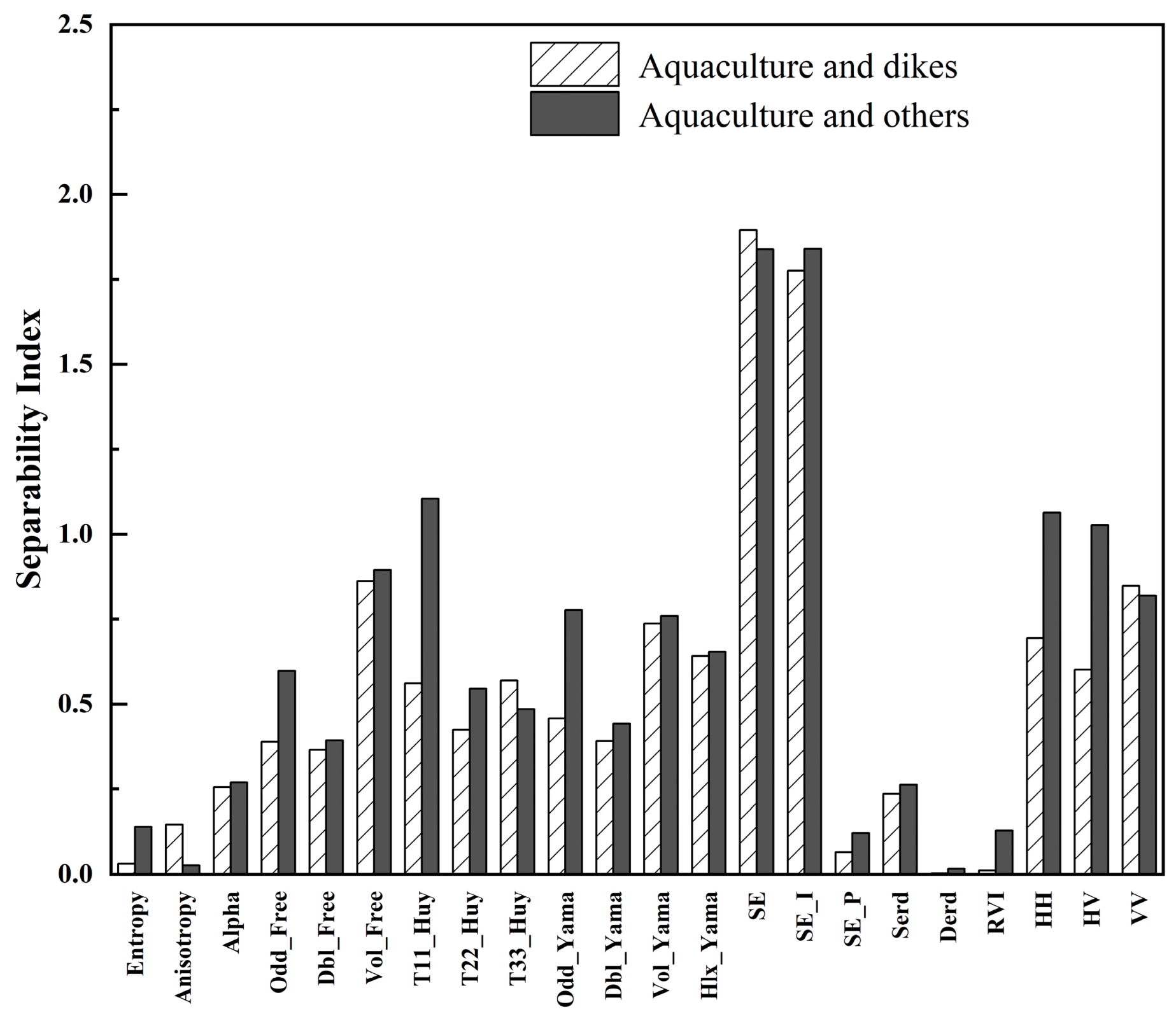
4.2. Separability of Polarimetric Features and Feature Optimisation

The separability index (SI) corresponding to 22 features was calculated, as shown in Figure 5, to intuitively evaluate the separability between two class pairs, namely, (1) aquacultures and dikes and (2) aquacultures and other (urban, vegetation and bare soil). The higher the SI value of a given feature, the better the separability between class pairs [45]. SE and SE_I, with SI values exceeding 1.5, can be used to separate the aquacultures from other classes (dikes and others) compared to other polarimetric features. Therefore, SE and SE_I are selected for the identification of aquaculture based on the feature separation criterion.

In addition, considering the regular shape and dense distribution of aquaculture ponds, eight texture features: mean, entropy, variance, contrast, second moment, homogeneity, dissimilarity and correlation, are applied to the two optimised features (SE and SE_I) to consider the spatial associations among pond objects. The SI values of the aforementioned texture features for SE and SE_I are shown in Figure 6. For texture features, the SI of Mean_SE and Mean_SE_I is higher than that of the other listed features and exceeds 1; therefore, Mean_SE and Mean_SE_I can be considered valuable auxiliary features for aquaculture extraction. Therefore, two polarimetric features (SE and SE_I) and two texture features (Mean_SE and Mean_SE_I) are selected as the optimal features suitable for aquaculture pond extraction.

4.3. The Results of Coastal Aquaculture Mapping and Accuracy Assessment

Figure 7 depicts the distribution of coastal aquacultures in the study area using the proposed method. The classification results were consistent with the ground truth in the study area. Coastal aquacultures are mainly densely distributed and located around rivers near the seaside.

To fully evaluate the performance of our proposed method, we compared our result with the results obtained using the SVM, RF, UNet, LinkNet and UNet++ methods. As shown in

Table 2. Accuracy assessment of different models (%).

Model	F1	IOU	Matching Rate	insF1
SVM	91.02	83.52	-	-
RF	91.30	83.99	-	-
UNet	94.45	89.49	47.96	70.83
LinkNet	94.40	89.40	38.64	62.00
UNet++	93.98	88.65	55.26	74.94
MCW (3BPR, 2BPR)	95.75	91.85	77.00	87.05

, our deep learning method achieved a higher extraction accuracy than machine learning methods in aquaculture extraction; the proposed method (MCW (3^BPR, 2^BPR)) yielded the highest F1 score of 95.75% and IOU of 91.85%, improvements of 1.77% and 3.2% compared with those of the UNet++ network. Moreover, the MCW (3^BPR, 2^BPR) method can accurately capture the shape of aquaculture objects, with the highest matching rate of 77.00%, which is 21.74% higher than that of UNet++. It is obvious that the proposed method performs better in instance segmentation with the highest InsF1 of 87.05%.

5. Discussion

5.1. Multiclass Segmentation Strategy during Marker Prediction

The predominant regions during the segmentation of aquacultures are the background, aquaculture interior (foreground) and areas between aquacultures (dikes), with intensity differences shown in Figure 8. The intensity of the dikes overlaps that of the aquacultures and background to some extent. The ordinary marker extraction process defines a final marker based on two categories: foreground and background. However, including the areas between aquacultures as part of the background may result in a certain overlap in the intensity distributions of the foreground and background, making the separation of pixels more difficult. In this study, we applied a multiclass segmentation strategy in the UNet++_m network to divide the intermediate markers into three categories (aquaculture, background and dike). The addition of the dike class contributed to separating the touching borders of the aquacultures and ensured the reliability of the marker prediction result obtained with the UNet++_m network. Then, the generated aquaculture class was selected as the marker result.

5.2. Impacts of Boundary Patch Refinement

As illustrated above, the proposed method consists of two independent UNet++ networks: UNet++_f for foreground prediction and UNet++_m for marker prediction. However, a low proportion of boundaries easily leads to an imbalance problem during instance segmentation, thus resulting in imprecise and coarse segmentation results. In this study, boundary patch refinement (BPR) is applied to both UNet++_f and UNet++_m (MCW (3^BPR, 2^BPR)) to improve the boundary quality through a crop-then-refine strategy. Additionally, three comparative experiments are conducted to evaluate the performance of the BPR strategy: UNet++-based marker-controlled watershed segmentation (MWC (3, 2)), UNet++-based marker-controlled watershed segmentation in which BPR is applied to UNet++_f (MCW (3, 2^BPR)) and UNet++-based marker-controlled watershed segmentation where BPR is applied to UNet++_m (MCW (3^BPR, 2)), as shown in

Table 3. Comparison experiments for the BPR strategy, where the best is in bold. Note that ‘√’ represents that the corresponding BPR strategy was used, and the meaning of ‘✕’ is the opposite.

Model	Boundary Patch Refinement		F1	IoU	MR	insF1
	UNet++m	UNet++f
MCW (3, 2)	✕	✕	95.47	91.34	64.12	81.11
MCW (3, 2BPR)	✕	√	95.59	91.55	70.33	84.12
MCW (3BPR, 2)	√	✕	95.74	91.83	74.87	86.12
MCW (3BPR, 2BPR)	√	√	95.75	91.85	77.00	87.05

. With the MCW framework, experiments using BPR for both the UNet++_m and UNet++_f models (the proposed MCW (3^BPR, 2^BPR)) achieve the highest extraction accuracy, with values of 95.75%, 91.85%, 77% and 87.05% for F1, IoU, MR and insF1, respectively. The F1 and IoU of the four MCW-based methods are over 95% and 91%, respectively. While the pixel-based metrics (F1 and IoU) of the ablation study and the proposed method are very similar, the improvements are even more significant in terms of the object-based metric (MR) and instance-based metric (insF1). For the MCW (3, 2) method, the MR and insF1 values are 64.12% and 81.11%, respectively. When the BPR is added to UNet++_f, MR and insF1 are improved to 70.33% and 80.12%, respectively. After introducing the BPR strategy into UNet++_m, MCW (3^BPR, 2) yields MR and insF1 improvements of 10.72% and 5.01%, respectively. The highest MR and insF1 (77% and 87.05%, respectively) are obtained by the method with BPR and the two UNet++ networks in the MCW framework (the proposed method). The result demonstrates the importance of performing boundary patch refinement with the two UNet++ subnetworks of the MCW framework; notably, the MR and insF1 values are increased by 12.88% and 5.94%, respectively, compared to those for MCW (3, 2).

To qualitatively detail the effect of the BPR framework on aquaculture extraction, we present the results of the ablation study in four representative areas, as shown in Figure 9. The results of MCW (3, 2) show obvious omissions for some small, shallow ponds. However, after adding the BPR strategy, the missing small ponds are successfully extracted, as shown in Figure 9b. Moreover, Figure 9a,d show two cases in which BPR has successfully considered the previously unextracted pond corners and edge areas in regular rectangles. Figure 9c shows the problem of oversegmentation that exists for MCW (3, 2). The BPR approach mitigates over-segmentation and improves the segmented shape of the compact small ponds. The results suggest that the BPR performs well in repairing and refining the boundaries of aquacultures. Some small aquacultures are very difficult to distinguish due to the speckle noise and limited resolution of SAR imagery. With the BPR strategy, we can identify more small aquacultures, and it also works well in separating adjacent ponds into individual objects and reducing the “adhesion” phenomenon.

5.3. Classification Performance of Single Classifiers and the Proposed Combined Model

We further compared the proposed MCW (3^BPR, 2^BPR) with several single classifiers, including two machine learning models (support vector machine and random forest) and three deep learning methods (UNet, LinkNet and UNet++), to assess its effectiveness. Figure 10 shows the regional aquaculture details in four typical areas. It can be intuitively seen that the SVM and RF results have many broken fragments (Figure 10b,c). The single deep learning models (UNet, LinkNet and UNet++) are also incapable of identifying small ponds with shallow water levels and misclassify some corners of large- and medium-sized ponds into nonaquaculture land types (Figure 10a,d). Comparatively, the classification results of our proposed method are consistent with the ground truth in the study area.

In terms of pixel-based metrics, the proposed MCW (3^BPR, 2^BPR) model achieves the highest F1 and IoU (95.75% and 91.85%, respectively). The F1 values of the aforementioned six models are all greater than 91, and the IoU is above 83 (Table 2), which proves the feasibility of using GF-3 polarimetric SAR data for this type of extraction work. Compared with the machine learning models, the deep learning methods yield significant improvements in F1 and IoU values. The deep learning models have achieved relatively high pixel-level accuracy; therefore, MR and insF1, which reflect the geometric quality and segmentation effect of extracted aquaculture ponds, are the key indicators that can be used to assess the performance of the model. Among the three single deep learning classifiers, UNet++ performs the best and yields the highest accuracy for aquaculture identification (55.26% for MR, 74.94% for insF1). Therefore, UNet++ is considered the best single deep learning method and is integrated with the MCW segmentation framework and BPR to form the proposed MCW (3^BPR, 2^BPR) model. As described in Table 2, the MR and insF1 values of the proposed method are increased by 21.74% and 12.11% compared with those of the single UNet++ network. The results show that the proposed MCW (3^BPR, 2^BPR) method in the study area achieves the highest F1 of 95.75%, IOU of 91.85%, MR of 77.00% and insF1 of 87.05%.

5.4. The Transferability and Robustness of the Integrated Framework

In this study, an MCW (3^BPR, 2^BPR) framework that integrates the MCW and BPR strategies is proposed to establish a refined and detailed aquaculture extraction scheme that includes precise and high-quality boundary information. To evaluate the transferability and robustness of the MCW (3^BPR, 2^BPR) framework, we extract aquaculture information with the MCW (3^BPR, 2^BPR) framework using three deep learning models (

Table 4. Results of applying the framework to different deep learning models, where the best is in bold.

Model	Model	F1	IoU	MR	insF1
Single model	UNet++	93.98	88.65	55.26	74.94
	UNet	94.45	89.49	47.96	70.83
	LinkNet	94.40	89.4	38.64	62.00
MCW (3BPR, 2BPR)	UNet++	95.75	91.85	77.00	87.05
	UNet	95.17	90.79	75.68	87.12
	LinkNet	94.99	90.46	71.42	84.07

). For three single deep learning models, the pixel-level precision F1 and IoU values are as high as 93 and 88, respectively, but the values of object-oriented precision MR and instance segmentation precision insF1 are relatively low. When the MCW (3^BPR, 2^BPR) framework is added, F1 and IoU slightly increase; notably, the MR and insF1 values for UNet++, UNet and LinkNet are improved by 21.74% and 12.11%, 27.72% and 16.29% and 32.78% and 22.07%, respectively. The highest F1, IoU, MR and insF1 (95.75%, 91.85%, 77.00% and 87.05%, respectively) are obtained with MCW (3^BPR, 2^BPR) based on UNet++ (the proposed method). This result demonstrates the importance of MCW (3^BPR, 2^BPR), as MR and insF1 are greatly improved by adding the proposed framework. Deep learning is a method that facilitates the accurate extraction of aquaculture ponds, and the proposed MCW (3^BPR, 2^BPR) framework can further improve the geometric quality and segmentation effect of aquaculture objects, thereby solving a series of boundary problems, such as incompleteness, fragmentation and adhesion. Since the framework achieves good results based on the aforementioned three deep learning models, the MCW (3^BPR, 2^BPR) framework is confirmed to be applicable and transferable.

6. Conclusions

In this study, we make the first attempt to explore the potential of deep learning based on GF-3 imagery for aquaculture extraction in coastal areas. We propose a generalised combinatorial model called MCW (3^BPR, 2^BPR), which is confirmed to be suitable for a variety of deep learning methods (UNet++, UNet and LinkNet). It combines an MCW segmentation framework with deep learning networks, in which a BPR postprocessing strategy is employed, and obtains high-precision aquaculture pond results in coastal areas using high-resolution GaoFen-3 polarimetric SAR remote sensing images. Compared with traditional methods, the following conclusions can be drawn.

(1)

GF-3 data contain rich and valuable surface scattering information and can thus be used for aquaculture extraction. A total of 22 features were obtained from four typical polarimetric segmentations and other polarimetric parameters. The separability index (SI) of all the features was calculated, and four features were optimised: SE, SE_I, SE_Mean and SE_I_Mean.

(2)

Compared with traditional machine learning methods, the introduction of deep learning methods greatly improved the extraction accuracy, with F1 greater than 94% and the IoU greater than 88%. In addition, compared with those of the UNet++ network alone, the F1, IOU, MR and insF1 of UNet++-based MCW (3^BPR, 2^BPR) (the proposed method) were improved by 1.7%, 3.2%, 21.74% and 12.11%, respectively.

(3)

The BPR postprocessing method optimised the extraction of boundary information for the aquaculture ponds, eliminating the error, omission and adhesion issues at the boundaries (dikes and dams). Notably, the MR and insF1 values increased by 12.88% and 5.94%, respectively.

(4)

The proposed MCW (3^BPR, 2^BPR) framework in this paper is not only applicable to UNet++ but also applicable to other deep learning models, such as LinkNet and UNet, and can obtain high-quality results. It was further confirmed that the MCW (3^BPR, 2^BPR) framework has certain robustness and universality.

GF-3 remote sensing images contain rich polarimetric information and can be used as an important data source for aquaculture extraction. The proposed MCW (3^BPR, 2^BPR) framework is devoted to enhancing boundary accuracy and preserving detailed information in the edge areas around aquacultures.

References

1. FAO. The State of World Fisheries and Aquaculture 2018-Meeting the Sustainable Development Goals; FAO: Rome, Italy, 2018; Volume 61, ISBN 9789251305621. [Google Scholar]
2. Alexandridis, T.K.; Topaloglou, C.A.; Lazaridou, E.; Zalidis, G.C. The performance of satellite images in mapping aquacultures. Ocean Coast. Manag. 2008, 51, 638–644. [Google Scholar] [CrossRef]
3. Sun, Z.; Luo, J.; Yang, J.; Yu, Q.; Zhang, L.; Xue, K.; Lu, L. Nation-scale mapping of coastal aquaculture ponds with sentinel-1 SAR data using google earth engine. Remote Sens. 2020, 12, 3086. [Google Scholar] [CrossRef]
4. Duan, Y.; Li, X.; Zhang, L.; Liu, W.; Liu, S.; Chen, D.; Ji, H. Detecting spatiotemporal changes of large-scale aquaculture ponds regions over 1988–2018 in Jiangsu Province, China using Google Earth Engine. Ocean Coast. Manag. 2020, 188, 105144. [Google Scholar] [CrossRef]
5. Duan, Y.; Tian, B.; Li, X.; Liu, D.; Sengupta, D.; Wang, Y.; Peng, Y. Tracking changes in aquaculture ponds on the China coast using 30 years of Landsat images. Int. J. Appl. Earth Obs. Geoinf. 2021, 102, 102383. [Google Scholar] [CrossRef]
6. Liu, Y.; Wang, Z.; Yang, X.; Zhang, Y.; Yang, F.; Liu, B.; Cai, P. Satellite-based monitoring and statistics for raft and cage aquaculture in China’s offshore waters. Int. J. Appl. Earth Obs. Geoinf. 2020, 91, 102118. [Google Scholar] [CrossRef]
7. Fu, Y.; Ye, Z.; Deng, J.; Zheng, X.; Huang, Y.; Yang, W.; Wang, Y.; Wang, K. Finer resolution mapping of marine aquaculture areas using world view-2 imagery and a hierarchical cascade convolutional neural network. Remote Sens. 2019, 11, 1678. [Google Scholar] [CrossRef]
8. Peng, Y.; Sengupta, D.; Duan, Y.; Chen, C.; Tian, B. Accurate mapping of Chinese coastal aquaculture ponds using biophysical parameters based on Sentinel-2 time series images. Mar. Pollut. Bull. 2022, 181, 113901. [Google Scholar] [CrossRef]
9. Yu, Z.; Di, L.; Rahman, M.S.; Tang, J. Fishpond mapping by spectral and spatial-based filtering on google earth engine: A case study in singra upazila of Bangladesh. Remote Sens. 2020, 12, 2692. [Google Scholar] [CrossRef]
10. Duan, Y.; Li, X.; Zhang, L.; Chen, D.; Liu, S.; Ji, H. Mapping national-scale aquaculture ponds based on the Google Earth Engine in the Chinese coastal zone. Aquaculture 2020, 520, 734666. [Google Scholar] [CrossRef]
11. Ren, C.; Wang, Z.; Zhang, Y.; Zhang, B.; Chen, L.; Xi, Y.; Xiao, X.; Doughty, R.B.; Liu, M.; Jia, M.; et al. Rapid expansion of coastal aquaculture ponds in China from Landsat observations during 1984–2016. Int. J. Appl. Earth Obs. Geoinf. 2019, 82, 101902. [Google Scholar] [CrossRef]
12. Stiller, D.; Ottinger, M.; Leinenkugel, P. Spatio-temporal patterns of coastal aquaculture derived from Sentinel-1 time series data and the full Landsat archive. Remote Sens. 2019, 11, 1707. [Google Scholar] [CrossRef]
13. Ottinger, M.; Clauss, K.; Kuenzer, C. Large-scale assessment of coastal aquaculture ponds with Sentinel-1 time series data. Remote Sens. 2017, 9, 440. [Google Scholar] [CrossRef]
14. Canty, M.J.; Nielsen, A.A.; Conradsen, K.; Skriver, H. Statistical analysis of changes in sentinel-1 time series on the Google earth engine. Remote Sens. 2020, 12, 46. [Google Scholar] [CrossRef]
15. Chen, Y.; He, X.; Xu, J.; Zhang, R.; Lu, Y. Scattering feature set optimization and polarimetric SAR classification using object-oriented RF-SFS algorithm in coastal wetlands. Remote Sens. 2020, 12, 407. [Google Scholar] [CrossRef]
16. Tu, C.; Li, P.; Li, Z.; Wang, H.; Yin, S.; Li, D.; Zhu, Q.; Chang, M.; Liu, J.; Wang, G. Synergetic classification of coastal wetlands over the yellow river delta with gf-3 full-polarization sar and zhuhai-1 ohs hyperspectral remote sensing. Remote Sens. 2021, 13, 4444. [Google Scholar] [CrossRef]
17. Schmitt, A.; Brisco, B. Wetland monitoring using the curvelet-based change detection method on polarimetric SAR imagery. Water 2013, 5, 1036–1051. [Google Scholar] [CrossRef]
18. Wan, J.; Wang, J.; Zhu, M. Water extraction from fully polarized sar based on combined polarization and texture features. Water 2021, 13, 3332. [Google Scholar] [CrossRef]
19. Fan, J.; Zhao, J.; Song, D.; Wang, X.; Wang, X.; Su, X. Marine floating raft aquaculture dynamic monitoring based on multi-source GF imagery. In Proceedings of the 2018 7th International Conference on Agro-Geoinformatics (Agro-Geoinformatics), Hangzhou, China, 6–9 August 2018; pp. 1–4. [Google Scholar]
20. Fan, J.; Zhao, J.; An, W.; Hu, Y. Marine floating raft aquaculture detection of GF-3 PolSAR images based on collective multikernel fuzzy clustering. IEEE J. Sel. Top. Appl. Earth Obs. Remote Sens. 2019, 12, 2741–2754. [Google Scholar] [CrossRef]
21. Ottinger, M.; Clauss, K.; Kuenzer, C. Opportunities and challenges for the estimation of aquaculture production based on earth observation data. Remote Sens. 2018, 10, 1076. [Google Scholar] [CrossRef]
22. Ottinger, M.; Clauss, K.; Huth, J.; Eisfelder, C.; Leinenkugel, P.; Kuenzer, C. Time series sentinel-1 SAR data for the mapping of aquaculture ponds in coastal Asia. In Proceedings of the International Geoscience and Remote Sensing Symposium (IGARSS), Valencia, Spain, 22–27 July 2018; pp. 9371–9374. [Google Scholar]
23. Cui, B.G.; Zhong, Y.; Fei, D.; Zhang, Y.H.; Liu, R.J.; Chu, J.L.; Zhao, J.H. Floating raft aquaculture area automatic extraction based on fully convolutional network. J. Coast. Res. 2019, 90, 86–94. [Google Scholar] [CrossRef]
24. Zeng, Z.; Wang, D.; Tan, W.; Yu, G.; You, J.; Lv, B.; Wu, Z. Rcsanet: A full convolutional network for extracting inland aquaculture ponds from high-spatial-resolution images. Remote Sens. 2021, 13, 92. [Google Scholar] [CrossRef]
25. Wei, S.; Zhang, H.; Wang, C.; Wang, Y.; Xu, L. Multi-temporal SAR data large-scale crop mapping based on U-net model. Remote Sens. 2019, 11, 68. [Google Scholar] [CrossRef]
26. Ronneberger, O.; Fischer, P.; Brox, T. U-net: Convolutional networks for biomedical image segmentation. In Proceedings of the Medical Image Computing and Computer-Assisted Intervention–MICCAI 2015: 18th International Conference, Munich, Germany, 5–9 October 2015; Proceedings, Part III 18. Springer International Publishing: Berlin/Heidelberg, Germany, 2015; pp. 234–241. [Google Scholar]
27. Zhang, Z.; Liu, Q.; Wang, Y. Road extraction by deep residual u-net. IEEE Geosci. Remote Sens. Lett. 2018, 15, 749–753. [Google Scholar] [CrossRef]
28. Wang, J.; Fan, J.; Wang, J. MDOAU-Net: A lightweight and robust deep learning model for SAR Image segmentation in aquaculture raft monitoring. IEEE Geosci. Remote Sens. Lett. 2022, 19, 1–5. [Google Scholar] [CrossRef]
29. Zhou, Z.; Rahman Siddiquee, M.M.; Tajbakhsh, N.; Liang, J. Unet++: A nested u-net architecture for medical image segmentation. In Proceedings of the Deep Learning in Medical Image Analysis and Multimodal Learning for Clinical Decision Support: 4th International Workshop, DLMIA 2018, and 8th International Workshop, ML-CDS 2018, Held in Conjunction with MICCAI 2018, Granada, Spain, 20 September 2018; Springer International Publishing: Berlin/Heidelberg, Germany, 2018; Volume 11045 LNCS, pp. 3–11. [Google Scholar]
30. Zhou, Z.; Siddiquee, M.M.R.; Tajbakhsh, N.; Liang, J. Unet++: Redesigning skip connections to exploit multiscale features in image segmentation. IEEE Trans. Med. Imaging 2019, 39, 1856–1867. [Google Scholar] [CrossRef] [PubMed]
31. Gaetano, R.; Masi, G.; Poggi, G.; Verdoliva, L.; Scarpa, G. Marker-controlled watershed-based segmentation of multiresolution remote sensing images. IEEE Trans. Geosci. Remote Sens. 2015, 53, 2987–3004. [Google Scholar] [CrossRef]
32. Yang, X.; Li, H.; Zhou, X. Nuclei segmentation using marker-controlled watershed, tracking using mean-shift, and Kalman filter in time-lapse microscopy. IEEE Trans. Circuits Syst. I Regul. Pap. 2006, 53, 2405–2414. [Google Scholar] [CrossRef]
33. Kim, E.; Park, S.; Hwang, S.; Moon, I.; Javidi, B. Deep learning-based phenotypic assessment of red cell storage lesions for safe transfusions. IEEE J. Biomed. Health Inform. 2021, 26, 1318–1328. [Google Scholar] [CrossRef]
34. Waldner, F.; Diakogiannis, F.I. Deep learning on edge: Extracting field boundaries from satellite images with a convolutional neural network. Remote Sens. Environ. 2020, 245, 111741. [Google Scholar] [CrossRef]
35. Hay, G.J.; Blaschke, T.; Marceau, D.J. A comparison of three image-object methods for the multiscale analysis of landscape structure. ISPRS J. Photogramm. Remote Sens. 2003, 57, 327–345. [Google Scholar] [CrossRef]
36. Xing, F.; Xie, Y.; Yang, L. An automatic learning-based framework for robust nucleus segmentation. IEEE Trans. Med. Imaging 2016, 35, 550–566. [Google Scholar] [CrossRef] [PubMed]
37. Chen, H.; Qi, X.; Yu, L.; Dou, Q.; Qin, J.; Heng, P.A. DCAN: Deep contour-aware networks for object instance segmentation from histology images. Med. Image Anal. 2017, 36, 135–146. [Google Scholar] [CrossRef] [PubMed]
38. Xie, L.; Qi, J.; Pan, L.; Wali, S. Integrating deep convolutional neural networks with marker-controlled watershed for overlapping nuclei segmentation in histopathology images. Neurocomputing 2020, 376, 166–179. [Google Scholar] [CrossRef]
39. Lux, F.; Matula, P. Cell segmentation by combining marker-controlled watershed and deep learning. arXiv 2020, arXiv:2004.01607. [Google Scholar]
40. Ju, A.; Wang, Z. A novel fully convolutional network based on marker-controlled watershed segmentation algorithm for industrial soot robot target segmentation. Evol. Intell. 2022, 1–18. [Google Scholar] [CrossRef]
41. Naylor, P.; Laé, M.; Reyal, F.; Walter, T. Segmentation of nuclei in histopathology images by deep regression of the distance map. IEEE Trans. Med. Imaging 2019, 38, 448–459. [Google Scholar] [CrossRef]
42. Zhu, Y.; Liu, K.; Myint, S.W.; Du, Z.; Li, Y.; Cao, J.; Liu, L.; Wu, Z. Integration of GF2 optical, GF3 SAR, and UAV data for estimating aboveground biomass of China’s largest artificially planted mangroves. Remote Sens. 2020, 12, 2039. [Google Scholar] [CrossRef]
43. Han, G.; Changcheng, W.; Guanya, W.; Jianjun, Z.; Yuqi, T.; Peng, S.; Ziwei, Z. A crop classification method integrating GF-3 PolSAR and Sentinel-2A optical data in the Dongting Lake Basin. Sensors 2018, 18, 3139. [Google Scholar] [CrossRef]
44. Shuai, G.; Zhang, J.; Basso, B.; Pan, Y.; Zhu, X.; Zhu, S.; Liu, H. Multi-temporal RADARSAT-2 polarimetric SAR for maize mapping supported by segmentations from high-resolution optical image. Int. J. Appl. Earth Obs. Geoinf. 2019, 74, 1–15. [Google Scholar] [CrossRef]
45. Mishra, P.; Singh, D. A statistical-measure-based adaptive land cover classification algorithm by efficient utilization ofbservables. IEEE Trans. Geosci. Remote Sens. 2014, 52, 2889–2900. [Google Scholar] [CrossRef]
46. Gupta, S.; Singh, D.; Kumar, S. An approach based on texture measures to classify the fully polarimetric SAR image. In Proceedings of the 9th International Conference on Industrial and Information Systems, ICIIS 2014, Gwalior, India, 15–17 December 2014; pp. 1–6. [Google Scholar]
47. Radars, P.; Data, A.T. Decision tree approach to classify the fully polarimetric RADARSAT-2 data. In Proceedings of the National Conference on Recent Advances in Electronics & Computer Engineering, RAECE-2015, Roorkee, India, 13–15 February 2015; pp. 318–323. [Google Scholar]
48. Ping, L.; Xin, X.; Hao, D.; Xu, D. Polarimetric SAR image feature selection and multi-layer SVM classification using divisibility index. J. Comput. Appl. 2018, 38, 132. [Google Scholar]
49. Mishra, P.; Singh, D.; Yamaguchi, Y. Land cover classification of PALSAR images by knowledge based decision tree classifier and supervised classifiers based on SAR observables. Prog. Electromagn. Res. B 2011, 30, 47–70. [Google Scholar] [CrossRef]
50. Li, Z.; Zuo, J.; Zhang, C.; Sun, Y. Pneumothorax image segmentation and prediction with UNet++ and MSOF strategy. In Proceedings of the 2021 IEEE International Conference on Consumer Electronics and Computer Engineering, ICCECE 2021, Guangzhou, China, 15–17 January 2021; pp. 710–713. [Google Scholar]
51. Yi, F.; Moon, I.; Javidi, B. Automated red blood cells extraction from holographic images using fully convolutional neural networks. Biomed. Opt. Express 2017, 8, 4466–4479. [Google Scholar] [CrossRef] [PubMed]
52. Yang, X.; Zhou, Y.; Zhang, X.; Li, R.; Yang, D. Accurate extraction of artificial pit-pond integrating edge features and semantic information. J. Geo-Inform. Sci. 2022, 24, 766–779. [Google Scholar] [CrossRef]
53. Cheng, B.; Liang, C.; Liu, X.; Liu, Y.; Ma, X.; Wang, G. Research on a novel extraction method using Deep Learning based on GF-2 images for aquaculture areas. Int. J. Remote Sens. 2020, 41, 3575–3591. [Google Scholar] [CrossRef]
54. Tang, C.; Chen, H.; Li, X.; Li, J.; Zhang, Z.; Hu, X. Look closer to segment better: Boundary patch refinement for instance segmentation. In Proceedings of the IEEE Computer Society Conference on Computer Vision and Pattern Recognition, Nashville, TN, USA, 19–25 June 2021; pp. 13926–13935. [Google Scholar]
55. Ding, L.; Tang, H.; Liu, Y.; Shi, Y.; Zhu, X.X.; Bruzzone, L. Adversarial shape learning for building extraction in VHR remote sensing images. IEEE Trans. Image Process. 2022, 31, 678–690. [Google Scholar] [CrossRef] [PubMed]
56. Xu, L.; Liu, Y.; Yang, P.; Chen, H.A.O.; Zhang, H.; Wang, D.A.N.; Zhang, X.I.N. HA U-Net: Improved model for building extraction from high resolution remote sensing imagery. IEEE Access 2021, 9, 101972–101984. [Google Scholar] [CrossRef]
57. Ma, X. Apollo: An adaptive parameter-wise diagonal quasi-newton method for nonconvex stochastic optimization. arXiv 2020, arXiv:2009.13586. [Google Scholar]
58. Loshchilov, I.; Hutter, F. SGDR: Stochastic gradient descent with warm restarts. arXiv 2016, arXiv:1608.03983. [Google Scholar]
Figure 1. Location of the study area.
Remotesensing 15 02246 g001
Figure 2. Overview of the proposed method.
Remotesensing 15 02246 g002
Figure 3. Architecture of UNet++.
Remotesensing 15 02246 g003
Figure 4. Overview of the boundary patch refinement framework. (a) The coarse segmentation results produced by a UNet++ instance segmentation model; (b) coarse patch extraction results for error-prone boundaries; (c) sparse error-prone boundary results obtained after filtering out some patches using Euclidean distance; (d) original polarisation feature image; (e) image patches of the error-prone boundaries; (f) filtered sparse error-prone boundary patches; (g) refined boundary patches; and (h) the final fusion results. The red box indicates the area where changes occur during the BPR processing.
Remotesensing 15 02246 g004
Figure 5. Separability index for polarimetric features.
Remotesensing 15 02246 g005
Figure 6. Separability index for texture features.
Remotesensing 15 02246 g006
Figure 7. Spatial distribution of coastal aquaculture in the study area based on the proposed algorithm: (a,c,d) large-scale aquaculture area, and (b) small-scale aquaculture area.
Remotesensing 15 02246 g007
Figure 8. Intensity distributions of three intermediate marker categories for four optimised features: SE (a), SE_I (b), SE_MEAN (c) and SE_I_MEAN (d).
Remotesensing 15 02246 g008
Figure 9. Comparison of aquaculture extraction details for four typical regions obtained in different BPR ablation experiments: (a) large-scale aquaculture area, and (bd) small-scale aquaculture area. The blue circles indicate areas with significant differences.
Remotesensing 15 02246 g009
Figure 10. The classification results for four typical regions (ad) in the study area using SVM, RF, UNet, LinkNet, UNet++ and MCW (3BPR, 2BPR), where the blue circles indicate areas with significant differences.
Remotesensing 15 02246 g010