

Spatial Distribution Analysis of Landslide Deformations and Land-Use Changes in the Three Gorges Reservoir Area by Using Interferometric and Polarimetric SAR

Abstract
:1. Introduction
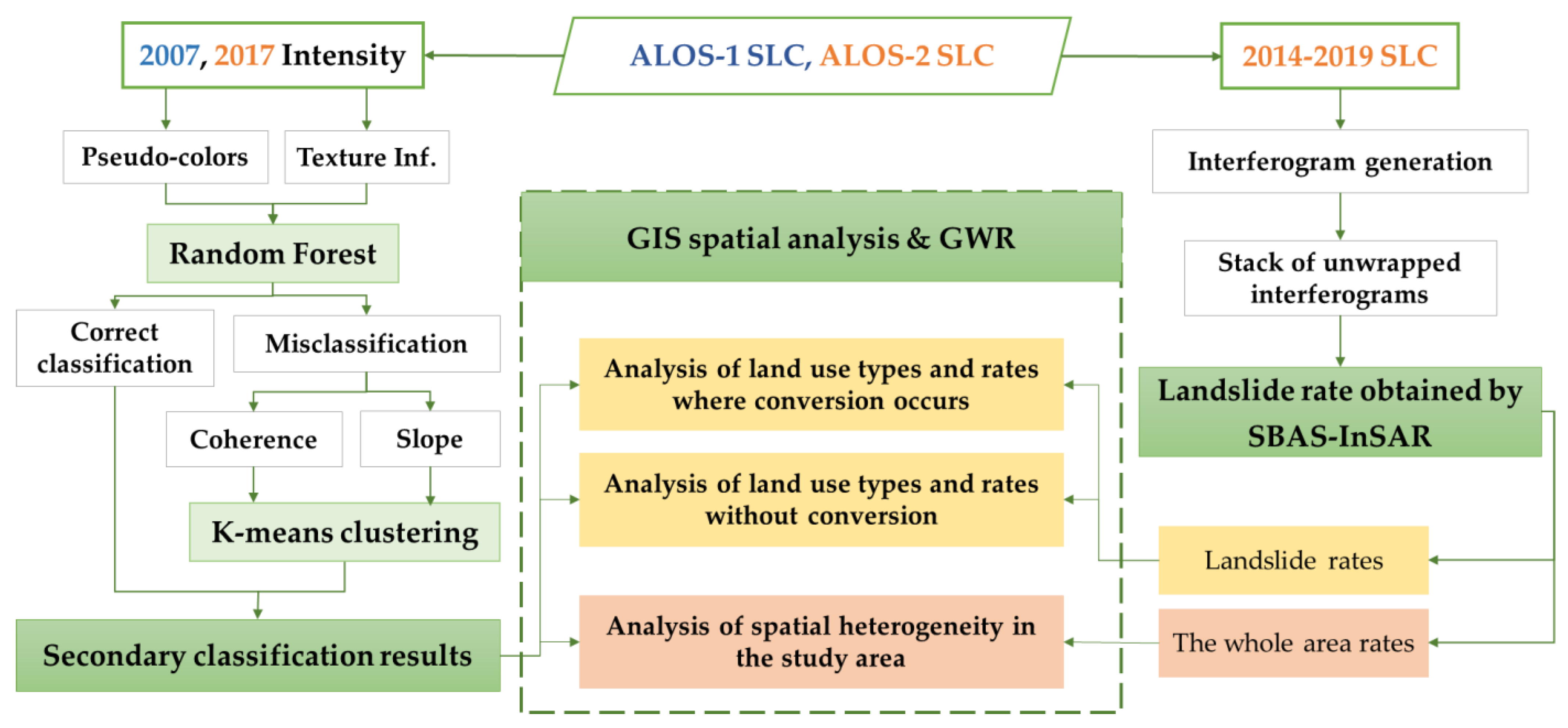
2. Methods
2.1. SBAS-InSAR Technology
2.2. The Secondary Classification Method and Accuracy Assessment
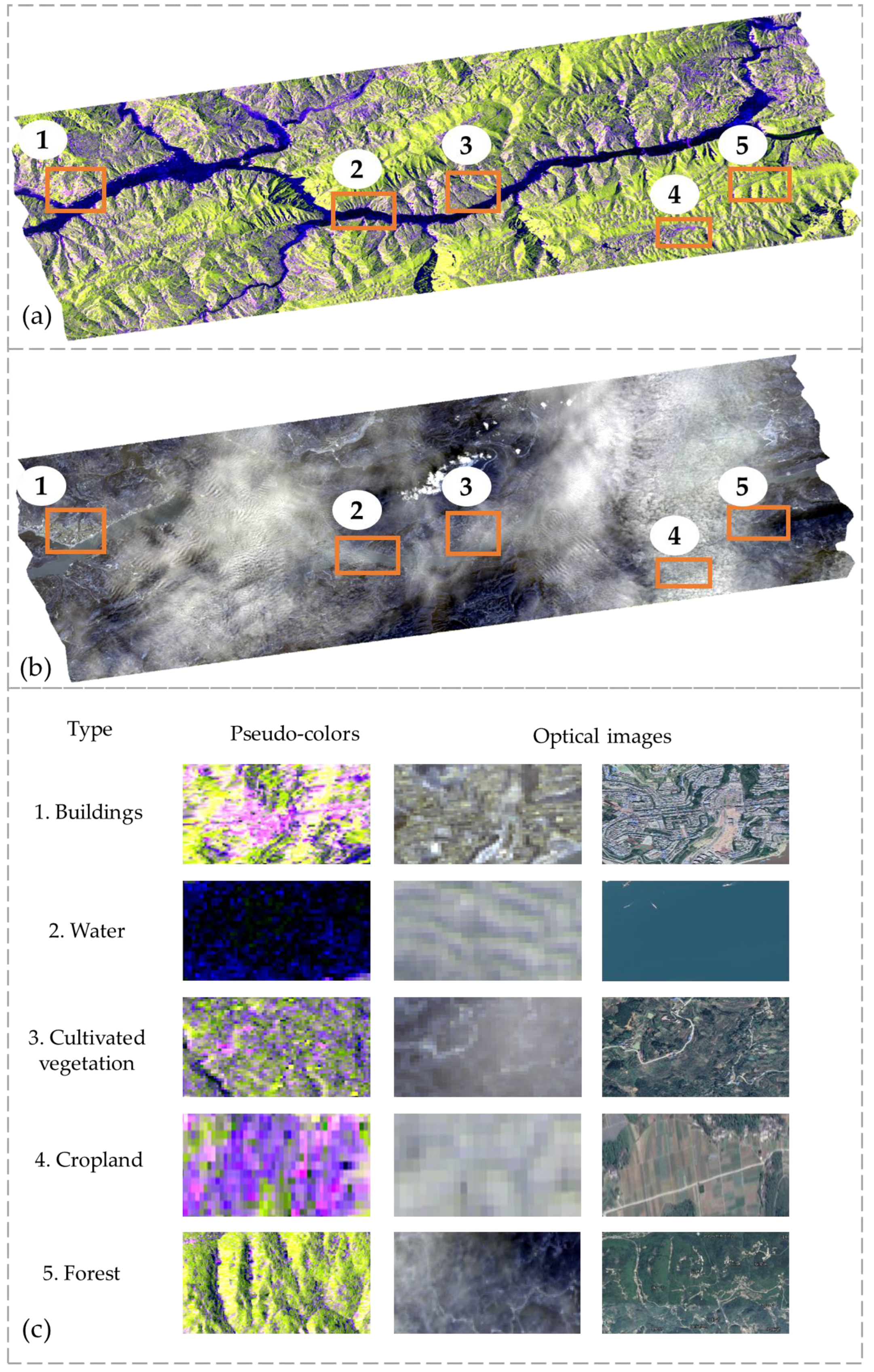
2.2.1. Secondary Classification with Dual-Polarization SAR Data
2.2.2. Accuracy Evaluation Index
2.3. Spatial Analysis
2.3.1. Data Preprocessing for Spatial Analysis
2.3.2. Spatial Analysis Method
3. Study Area and Data
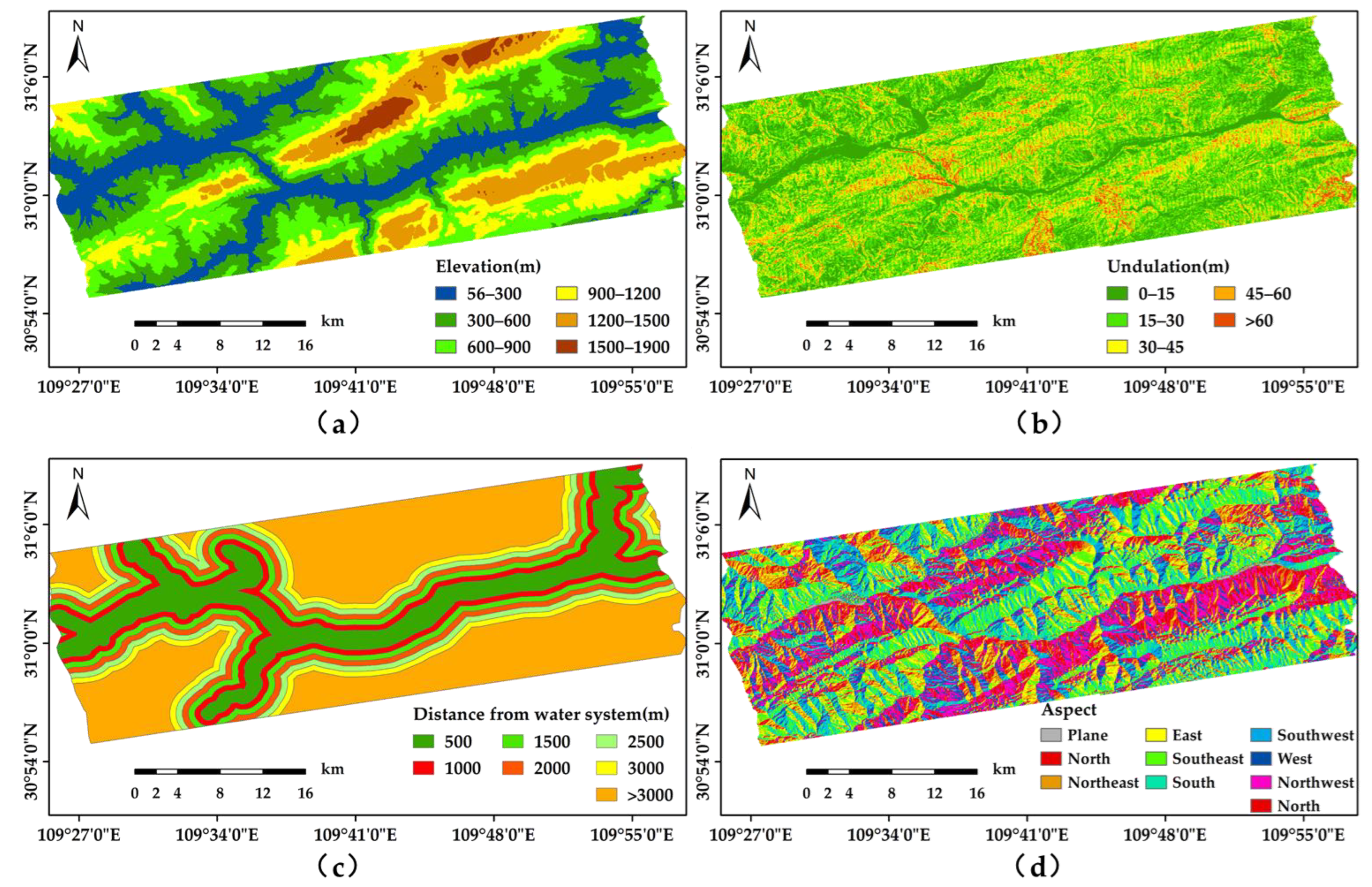
3.1. Overview of the Study Area
3.2. Data
4. Results
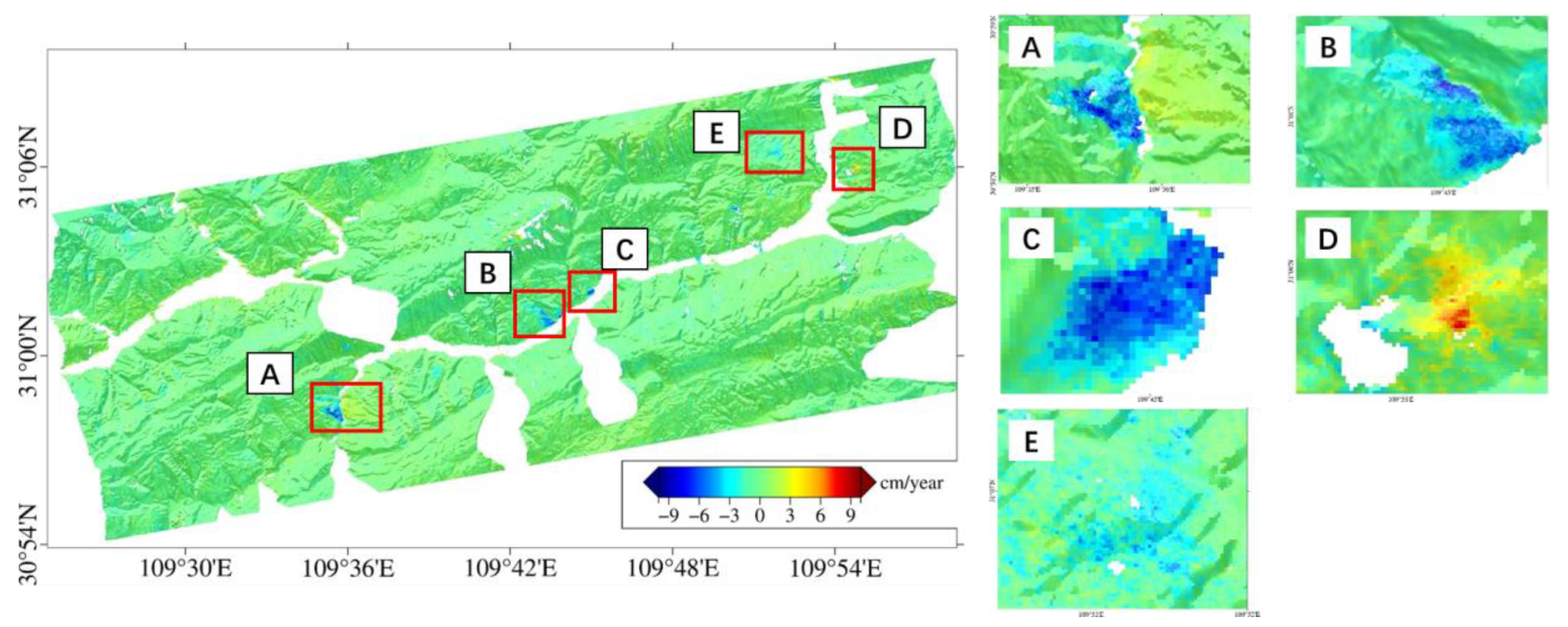
4.1. SBAS-InSAR to Monitor Landslide Deformation Rates
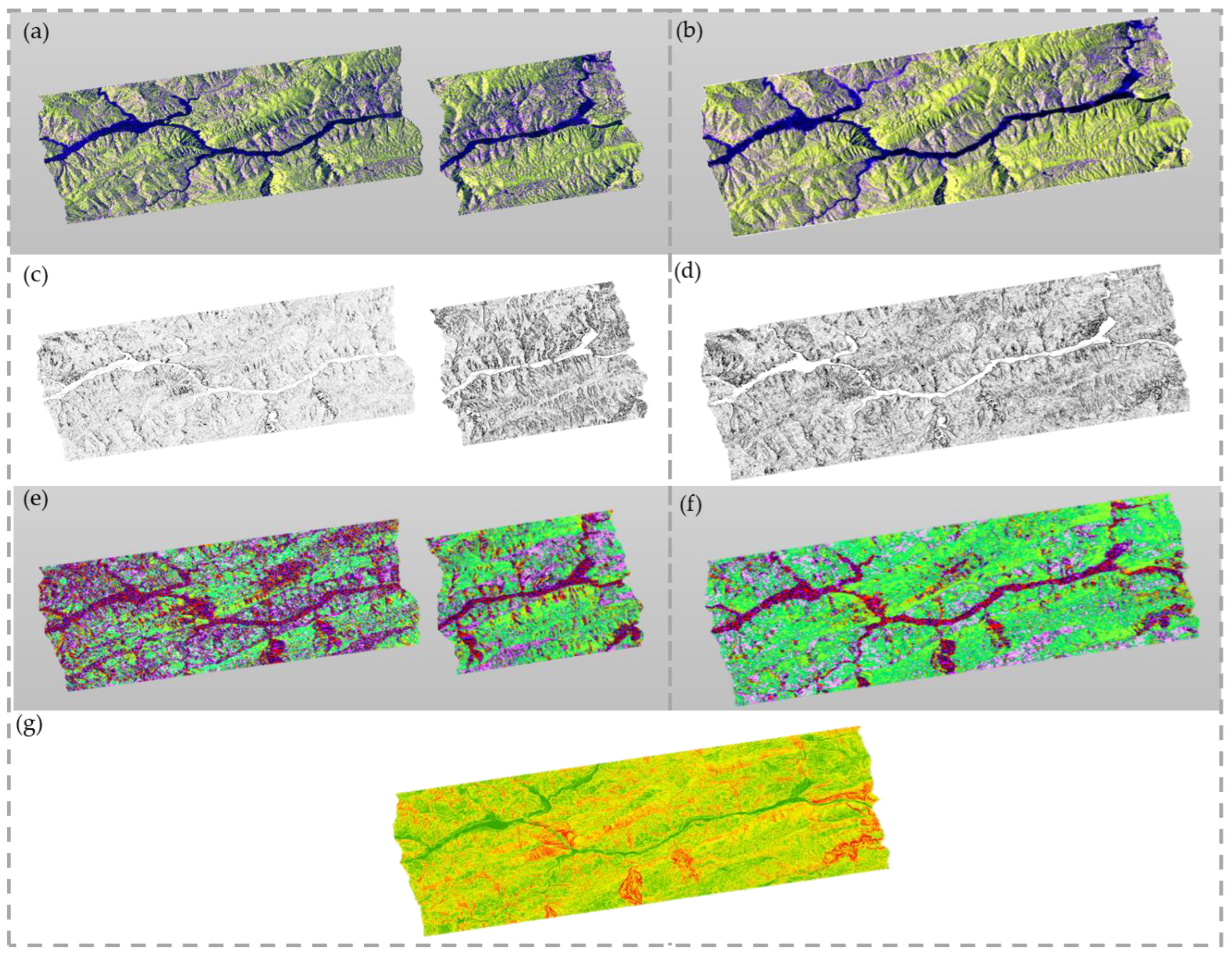
4.2. Secondary Classification Results and Accuracy Assessment
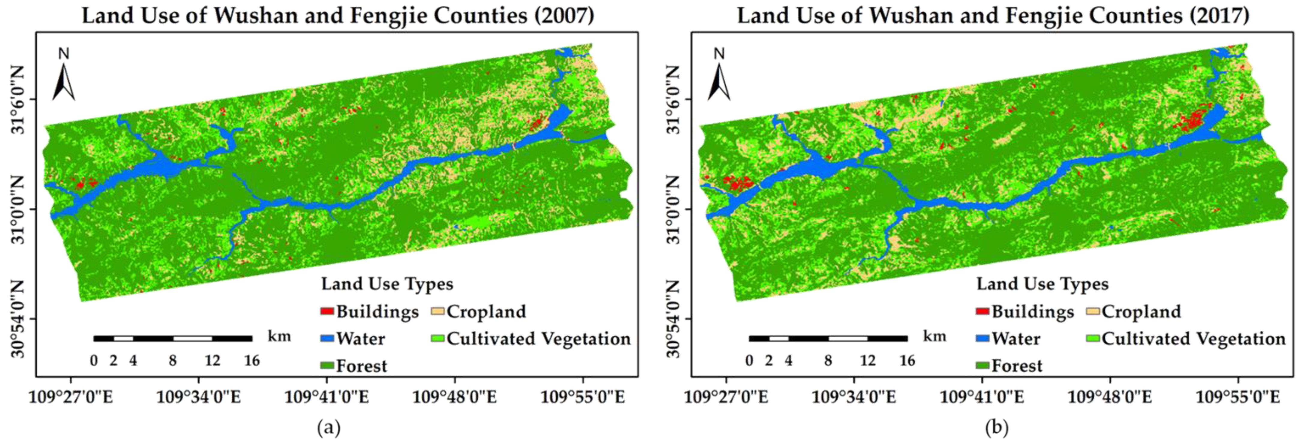
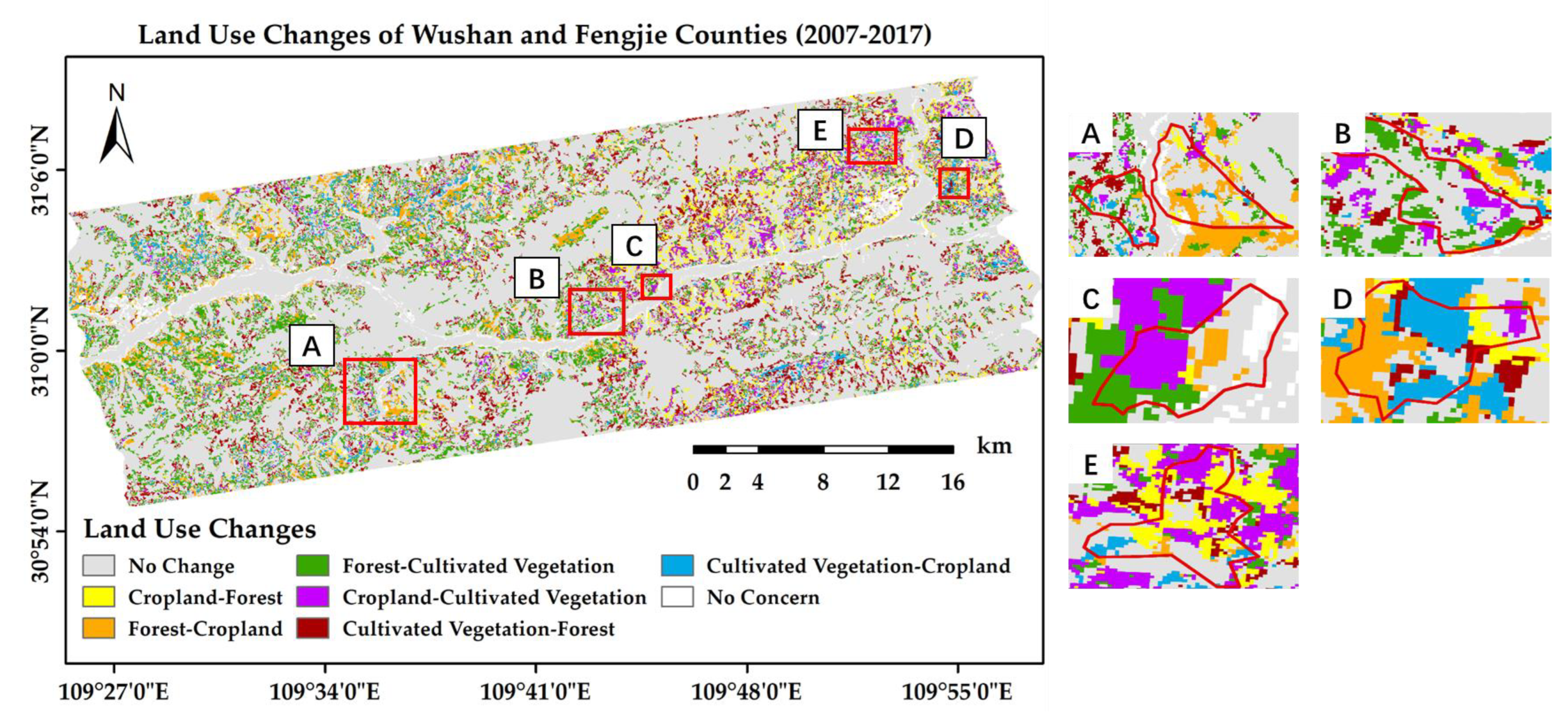
4.3. Land-Use Changes from 2007 to 2017
4.4. GIS Spatial Analysis with Landslide Deformations and Land-Use Changes
4.4.1. For Typical Landslide Areas with No Change in Land Use from 2007 to 2017
4.4.2. For Typical Landslide Areas with Land-Use Changes from 2007 to 2017
4.4.3. For the Typical Landslide Areas from 2007 to 2017
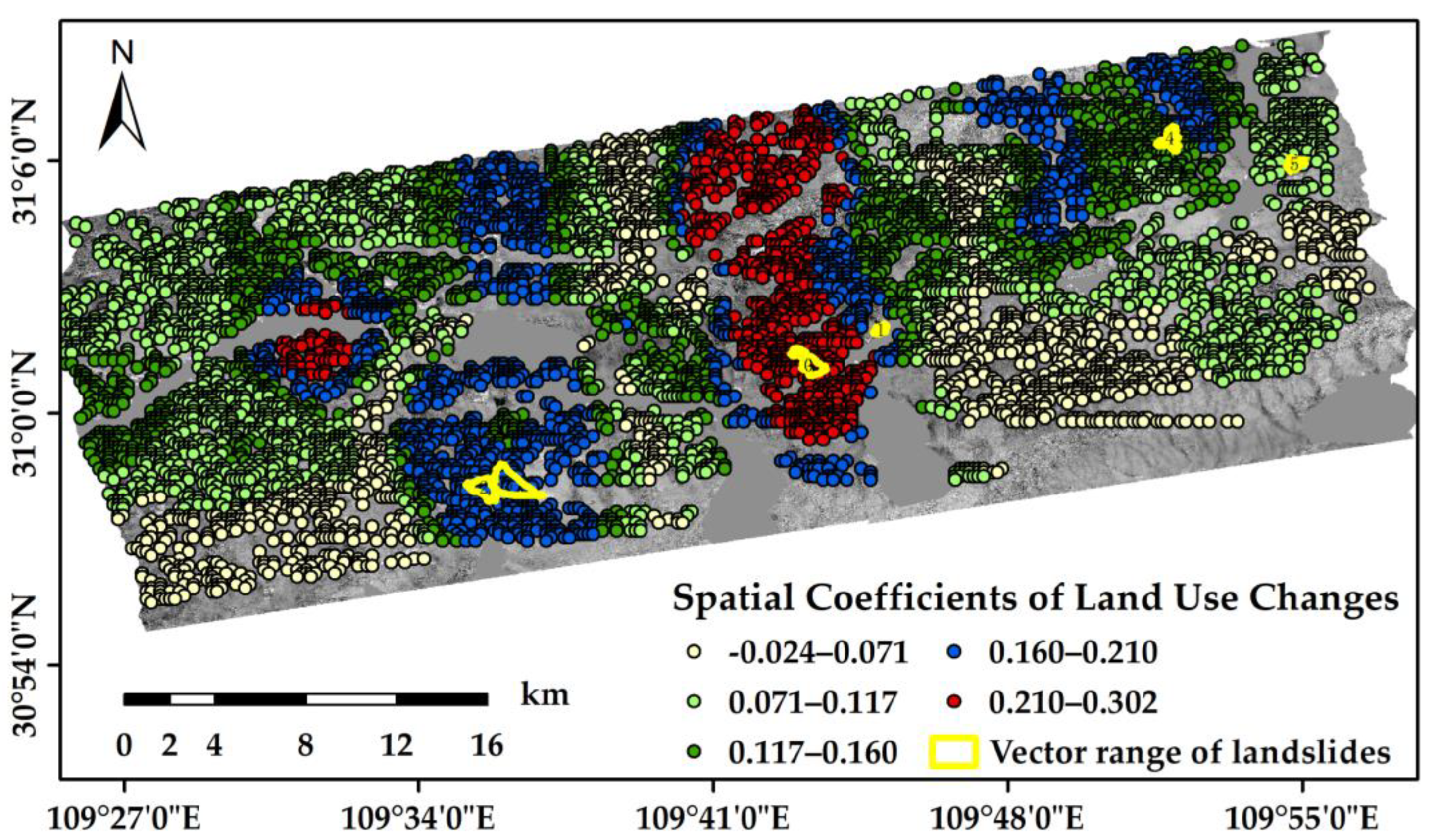
4.5. Spatial Heterogeneity Analysis with GWR
5. Discussion
5.1. Landslide Rates Monitored by SBAS-InSAR
5.2. Land-Use Classification with the Secondary Classification Method
5.3. Relationship between Landslide Deformation Rates and Land-Use Changes
6. Conclusions
- Land use classification in rugged areas cannot improve accuracy just by increasing feature data.
- It was possible to complete the classification by simplifying the multi-classification task into a binary classification task, and the classification accuracy obtained was higher and more reliable than that of only one classification.
- The land use types strongly influenced by the intensity of human activities can promote landslide deformation, such as cultivated vegetation.
- The landslide deformation rates were affected not only by the current land use type, but also by the historical land use type.
- Landslides were influenced by various internal and external factors. It was only when the geological conditions of landslides were met that the effects of land use and land use changes became apparent.
Author Contributions
Funding
Data Availability Statement
Acknowledgments
Conflicts of Interest
References
- Dai, F.; Lee, C.F.; Ngai, Y.Y. Landslide risk assessment and management: An overview. Eng. Geol. 2002, 64, 65–87. [Google Scholar] [CrossRef]
- Zhao, F.; Meng, X.; Zhang, Y.; Chen, G.; Su, X.; Yue, D. Landslide susceptibility mapping of karakorum highway combined with the application of SBAS-InSAR technology. Sensors 2019, 19, 2685. [Google Scholar] [CrossRef]
- Reichenbach, P.; Busca, C.; Mondini, A.; Rossi, M. The influence of land use change on landslide susceptibility zonation: The Briga catchment test site (Messina, Italy). Environ. Manag. 2014, 54, 1372–1384. [Google Scholar] [CrossRef] [PubMed]
- Huang, Y.; Zhao, L. Review on landslide susceptibility mapping using support vector machines. Catena 2018, 165, 520–529. [Google Scholar] [CrossRef]
- Tang, M.; Xu, K. Study on spatio-temporal evolution law and early warning and prediction of landslide. J. Rock Mech. Eng. 2008, 27, 1104–1112. [Google Scholar] [CrossRef]
- Luo, S.; Sarabandi, K.; Tong, L.; Pierce, L. Landslide prediction using soil moisture estimation derived from polarimetric Radarsat-2 data and SRTM. In 2016 IEEE International Geoscience and Remote Sensing Symposium (IGARSS); IEEE: New York, NY, USA, 2016; pp. 5386–5389. [Google Scholar]
- Qiang, X.; LU, H.; Weile, L.; Xiujun, D.; Chen, G. Types of Potential Landslide and Corresponding Identification Technologies. Geomat. Inf. Sci. Wuhan Univ. 2022, 47, 11. [Google Scholar] [CrossRef]
- Ferretti, A.; Prati, C.; Rocca, F. Permanent scatterers in SAR interferometry. IEEE Trans. Geosci. Remote Sens. 2001, 39, 8–20. [Google Scholar] [CrossRef]
- Berardino, P.; Fornaro, G.; Lanari, R.; Sansosti, E. A new algorithm for surface deformation monitoring based on small baseline differential SAR interferograms. IEEE 2002, 40, 2375–2383. [Google Scholar] [CrossRef]
- Ferretti, A.; Fumagalli, A.; Novali, F.; Prati, C.; Rocca, F.; Rucci, A. A new algorithm for processing interferometric data-stacks: SqueeSAR. IEEE Trans. Geosci. Remote Sens. 2011, 49, 3460–3470. [Google Scholar] [CrossRef]
- Guo, H.; Yi, B.; Yao, Q.; Gao, P.; Li, H.; Sun, J.; Zhong, C. Identification of Landslides in Mountainous Area with the Combination of SBAS-InSAR and Yolo Model. Sensors 2022, 22, 6235. [Google Scholar] [CrossRef]
- Yao, J.; Yao, X.; Liu, X. Landslide Detection and Mapping Based on SBAS-InSAR and PS-InSAR: A Case Study in Gongjue County, Tibet, China. Remote Sens. 2022, 14, 4728. [Google Scholar] [CrossRef]
- Umarhadi, D.A.; Widyatmanti, W.; Kumar, P.; Yunus, A.P.; Khedher, K.M.; Kharrazi, A.; Avtar, R. Tropical peat subsidence rates are related to decadal LULC changes: Insights from InSAR analysis. Sci. Total Environ. 2022, 816, 151561. [Google Scholar] [CrossRef]
- Wang, F.; Ding, Q.; Zhang, L.; Wang, M.; Wang, Q. Analysis of Land Surface Deformation in Chagan Lake Region Using TCPInSAR. Sustainability 2019, 11, 5090. [Google Scholar] [CrossRef]
- Gebremichael, E.; Sultan, M.; Becker, R.; El Bastawesy, M.; Cherif, O.; Emil, M. Assessing Land Deformation and Sea Encroachment in the Nile Delta: A Radar Interferometric and Inundation Modeling Approach. J. Geophys. Res. Solid Earth 2018, 123, 3208–3224. [Google Scholar] [CrossRef]
- Chaofan, Z.; Huili, G.; Beibei, C.; Jiwei, L.; Mingliang, G.; Feng, Z.; Wenfeng, C.; Yue, L. InSAR Time-Series Analysis of Land Subsidence under Different Land Use Types in the Eastern Beijing Plain, China. Remote Sens. 2017, 9, 380. [Google Scholar] [CrossRef]
- Minderhoud, P.; Coumou, L.; Erban, L.E.; Middelkoop, H.; Stouthamer, E.; Addink, E.A. The relation between land use and subsidence in the Vietnamese Mekong delta. Sci. Total Environ. 2018, 634, 715–726. [Google Scholar] [CrossRef]
- Abidin, H.Z.; Andreas, H.; Gumilar, I.; Fukuda, Y.; Pohan, Y.E.; Deguchi, T. Land subsidence of Jakarta (Indonesia) and its relation with urban development. Nat. Hazards 2011, 59, 1753–1771. [Google Scholar] [CrossRef]
- Han, Y.; Zou, J.; Lu, Z.; Qu, F.; Kang, Y.; Li, J. Ground deformation of wuhan, china, revealed by multi-temporal insar analysis. Remote Sens. 2020, 12, 3788. [Google Scholar] [CrossRef]
- Wang, Z.; Liu, Y.; Zhang, Y.; Liu, Y.; Wang, B.; Zhang, G. Spatially Varying Relationships between Land Subsidence and Urbanization: A Case Study in Wuhan, China. Remote Sens. 2022, 14, 291. [Google Scholar] [CrossRef]
- Maraun, D.; Knevels, R.; Mishra, A.N.; Truhetz, H.; Bevacqua, E.; Proske, H.; Zappa, G.; Brenning, A.; Petschko, H.; Schaffer, A.; et al. A severe landslide event in the Alpine foreland under possible future climate and land-use changes. Commun. Earth Environ. 2022, 3, 87. [Google Scholar] [CrossRef]
- Idham, R.M.; Kure, S.; Januriyadi, N.F.; Farid, M.; Udo, K.; Kazama, S.; Koshimura, S. Future projection of flood inundation considering land-use changes and land subsidence in Jakarta, Indonesia. Hydrol. Res. Lett. 2017, 11, 99–105. [Google Scholar] [CrossRef]
- Zhuo, G.; Dai, K.; Huang, H.; Li, S.; Shi, X.; Feng, Y.; Li, T.; Dong, X.; Deng, J. Evaluating Potential Ground Subsidence Geo-Hazard of Xiamen Xiang'an New Airport on Reclaimed Land by SAR Interferometry. Sustainability 2020, 12, 6991. [Google Scholar] [CrossRef]
- Fell, R.; Corominas, J.; Bonnard, C.; Cascini, L.; Leroi, E.; Savage, W.Z. Guidelines for landslide susceptibility, hazard and risk zoning for land use planning. Eng. Geol. 2008, 102, 85–98. [Google Scholar] [CrossRef]
- Dou, J.; Yamagishi, H.; Pourghasemi, H.R.; Yunus, A.P.; Song, X.; Xu, Y.; Zhu, Z. An integrated artificial neural network model for the landslide susceptibility assessment of Osado Island, Japan. Nat. Hazards 2015, 78, 1749–1776. [Google Scholar] [CrossRef]
- Li, C.; Wang, J.; Wang, L.; Hu, L.; Gong, P. Comparison of Classification Algorithms and Training Sample Sizes in Urban Land Classification with Landsat Thematic Mapper Imagery. Remote Sens. 2013, 6, 964. [Google Scholar] [CrossRef]
- Karalas, K.; Tsagkatakis, G.; Zervakis, M.; Tsakalides, P. Land Classification Using Remotely Sensed Data: Going Multilabel. IEEE Trans. Geosci. Remote Sens. 2016, 54, 3548–3563. [Google Scholar] [CrossRef]
- Merchant, M.A.; Obadia, M.; Brisco, B.; DeVries, B.; Berg, A. Applying Machine Learning and Time-Series Analysis on Sentinel-1A SAR/InSAR for Characterizing Arctic Tundra Hydro-Ecological Conditions. Remote Sens. 2022, 14, 1123. [Google Scholar] [CrossRef]
- Gao, W.; Yang, J.; Ma, W. Land Cover Classification for Polarimetric SAR Images Based on Mixture Models. Remote Sens. 2014, 6, 3770–3790. [Google Scholar] [CrossRef]
- Salehi, M.; Sahebi, M.R.; Maghsoudi, Y. Improving the Accuracy of Urban Land Cover Classification Using Radarsat-2 PolSAR Data. IEEE J. Sel. Top. Appl. Earth Obs. Remote Sens. 2014, 7, 1394–1401. [Google Scholar] [CrossRef]
- Alberga, V. A study of land cover classification using polarimetric SAR parameters. Int. J. Remote Sens. 2007, 28, 3851–3870. [Google Scholar] [CrossRef]
- Qi, Z.; Yeh, G.O.; Xia, L.; Zheng, L. A novel algorithm for land use and land cover classification using RADARSAT-2 polarimetric SAR data. Remote Sens. Environ. 2012, 118, 21–39. [Google Scholar] [CrossRef]
- Breiman, L. Random forests. Mach. Learn. 2001, 45, 5–32. [Google Scholar] [CrossRef]
- Macqueen, J. Some methods for classification and analysis of multivariate observations. In Proceedings of the Fifth Berkeley Symposium on Mathematical Statistics and Probability, Volume 1: Statistics; University of California Press: Berkeley, CA, USA, 1967. [Google Scholar]
- Fotheringham, A.S.; Brunsdon, C. Local Forms of Spatial Analysis. Geogr. Anal. 1999, 31, 340–358. [Google Scholar] [CrossRef]
- European Space Agency, Sinergise. Copernicus Global Digital Elevation Model; OpenTopography: La Jolla, CA, USA, 2021. [Google Scholar] [CrossRef]
- Karra, K.; Kontgis, C.; Statman-Weil, Z.; Mazzariello, J.C.; Mathis, M.; Brumby, S.P. Global land use/land cover with Sentinel 2 and deep learning. In Proceedings of the 2021 IEEE International Geoscience and Remote Sensing Symposium IGARSS, Brussels, Belgium, 11–16 July 2021; pp. 4704–4707. [Google Scholar]
- Yang, J.; Huang, X. The 30 m annual land cover dataset and its dynamics in China from 1990 to 2019. Earth Syst. Sci. Data 2021, 13, 3907–3925. [Google Scholar] [CrossRef]
- Zhu, J.; Li, Z.; Hu, J. Research progress and methods of InSAR for deformation monitoring. Acta Geod. Cartogr. Sin. 2017, 46, 1717. [Google Scholar] [CrossRef]


| Sensor | Date | Counts | SLC Thumbnails | Resolution (m) | Coverage | |
|---|---|---|---|---|---|---|
| HH | HV | |||||
| ALOS-1 | 2007 | 1 | 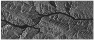 | 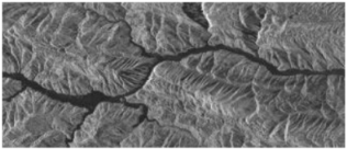 | 9 (range) × 3 (azimuth) | Fengjie County |
| 2007 | 1 | 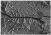 | 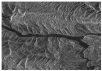 | Wushan County | ||
| ALOS-2 | 2014–2019 | 11 |  |  | 4 (range) × 3 (azimuth) | Fengjie and Wushan County |
| Name | Method | Classification Accuracy of Each Type(%) | OA (%) | Kappa (%) | ||||
|---|---|---|---|---|---|---|---|---|
| Buildings | Forest | Water | Cropland | Cultivated Vegetation | ||||
| Validation Area 1 | Comparison Method 1 | 89.63 | 76.03 | 100.00 | 84.70 | 83.70 | 82.29 | 74.72 |
| Comparison Method 2 | 99.67 | 78.88 | 100.00 | 91.16 | 88.58 | 86.12 | 80.33 | |
| Comparison Method 3 | 96.57 | 64.56 | 99.94 | 96.88 | 89.32 | 78.97 | 71.50 | |
| Secondary Classification | 84.45 | 95.80 | 99.94 | 98.07 | 89.00 | 94.44 | 91.59 | |
| Validation Area 2 | Comparison Method 1 | 81.35 | 40.18 | 99.92 | —— | —— | 87.38 | 78.14 |
| Comparison Method 2 | 97.21 | 70.44 | 99.92 | —— | —— | 96.02 | 93.02 | |
| Comparison Method 3 | 81.74 | 35.33 | 99.92 | —— | —— | 87.04 | 77.46 | |
| Secondary Classification | 90.62 | 89.83 | 99.96 | —— | —— | 95.52 | 92.29 | |
| 2007 | 2017 | |||||
|---|---|---|---|---|---|---|
| Buildings | Water | Forest | Cropland | Cultivated Vegetation | Total | |
| Buildings | 0.15 | 0.01 | 0.17 | 0.04 | 0.01 | 0.39 |
| Water | 0.00 | 4.88 | 0.17 | 0.13 | 0.04 | 5.23 |
| Forest | 0.41 | 0.83 | 53.65 | 3.99 | 9.46 | 68.33 |
| Cropland | 0.13 | 0.10 | 3.42 | 3.11 | 2.67 | 9.43 |
| Cultivated Vegetation | 0.05 | 0.02 | 6.65 | 2.29 | 7.61 | 16.62 |
| Total | 0.74 | 5.85 | 64.06 | 9.55 | 19.79 | 100.00 |
| 2007 | 2017 | |||||
|---|---|---|---|---|---|---|
| Buildings | Water | Forest | Cropland | Cultivated Vegetation | Total | |
| Buildings | 0.00 | 0.00 | 0.74 | 0.29 | 0.00 | 1.03 |
| Water | 0.00 | 1.86 | 0.26 | 0.19 | 0.13 | 2.45 |
| Forest | 0.00 | 0.97 | 11.18 | 12.32 | 9.64 | 34.11 |
| Cropland | 0.00 | 0.36 | 7.49 | 17.99 | 7.87 | 33.72 |
| Cultivated Vegetation | 0.00 | 0.00 | 4.34 | 5.76 | 18.59 | 28.70 |
| Total | 0.00 | 3.20 | 24.02 | 36.55 | 36.24 | 100.00 |
| Analysis Items | Variables | Sample Size | Mean Velocity (cm/year) | Statistics | p-Value | Effect Amount |
|---|---|---|---|---|---|---|
| Velocity | Cultivated Vegetation | 1308 | 3.47 | 1362.433 | 0.000 *** | 0.019 |
| Forest | 572 | 1.35 | ||||
| Cropland | 1322 | 1.54 | ||||
| Total | 3202 | - |
| Type 1 | Type 2 | Type 1 Rate | Type 2 Rate | 2017 Rate |
|---|---|---|---|---|
| Forest | Cropland | 1.35 | 1.54 | 1.58 |
| Forest | Cultivated Vegetation | 1.35 | 3.47 | 3.36 |
| Cropland | Forest | 1.54 | 1.35 | 1.59 |
| Cropland | Cultivated Vegetation | 1.54 | 3.47 | 2.73 |
| Cultivated Vegetation | Forest | 3.47 | 1.35 | 2.79 |
| Cultivated Vegetation | Cropland | 3.47 | 1.54 | 2.30 |
| Correlation Coefficient | 0.15 | 0.70 | 1.00 | |
| Velocity (cm/year) | Type after Change | |||
|---|---|---|---|---|
| Forest | Cropland | Cultivated Vegetation | ||
| Type before Change | Forest | 1.35 | 1.58 | 3.36 |
| Cropland | 1.59 | 1.54 | 2.73 | |
| Cultivated Vegetation | 2.79 | 2.30 | 3.47 | |
| Mean | 1.91 | 1.81 | 3.19 | |
Disclaimer/Publisher’s Note: The statements, opinions and data contained in all publications are solely those of the individual author(s) and contributor(s) and not of MDPI and/or the editor(s). MDPI and/or the editor(s) disclaim responsibility for any injury to people or property resulting from any ideas, methods, instructions or products referred to in the content. |
© 2023 by the authors. Licensee MDPI, Basel, Switzerland. This article is an open access article distributed under the terms and conditions of the Creative Commons Attribution (CC BY) license (https://creativecommons.org/licenses/by/4.0/).
Share and Cite
Hu, J.; Yu, Y.; Gui, R.; Zheng, W.; Guo, A. Spatial Distribution Analysis of Landslide Deformations and Land-Use Changes in the Three Gorges Reservoir Area by Using Interferometric and Polarimetric SAR. Remote Sens. 2023, 15, 2302. https://doi.org/10.3390/rs15092302
Hu J, Yu Y, Gui R, Zheng W, Guo A. Spatial Distribution Analysis of Landslide Deformations and Land-Use Changes in the Three Gorges Reservoir Area by Using Interferometric and Polarimetric SAR. Remote Sensing. 2023; 15(9):2302. https://doi.org/10.3390/rs15092302
Chicago/Turabian StyleHu, Jun, Yana Yu, Rong Gui, Wanji Zheng, and Aoqing Guo. 2023. "Spatial Distribution Analysis of Landslide Deformations and Land-Use Changes in the Three Gorges Reservoir Area by Using Interferometric and Polarimetric SAR" Remote Sensing 15, no. 9: 2302. https://doi.org/10.3390/rs15092302
APA StyleHu, J., Yu, Y., Gui, R., Zheng, W., & Guo, A. (2023). Spatial Distribution Analysis of Landslide Deformations and Land-Use Changes in the Three Gorges Reservoir Area by Using Interferometric and Polarimetric SAR. Remote Sensing, 15(9), 2302. https://doi.org/10.3390/rs15092302