ISAR Imaging of Non-Stationary Moving Target Based on Parameter Estimation and Sparse Decomposition

Abstract

This paper studies the inverse synthetic aperture radar imaging problem for a non-stationary moving target and proposes a non-search imaging method based on parameter estimation and sparse decomposition. The echoes received by radar can be thought of as consisting of chirp signals with varying chirp rates and center frequencies. Lv’s distribution (LVD) is introduced to accurately estimate these parameters. Considering their inherent sparsity, the signals are reconstructed via sparse representation using a redundant chirp dictionary. An efficient algorithm is developed to tackle the optimization problem for sparse decompositions. Then, by using the reconstructed data, adaptive joint time–frequency imaging techniques are employed to create high-quality images of the non-stationary moving target. Finally, the simulated experiments and measured data processing results confirm the proposed method’s validity.

1. Introduction

Inverse synthetic aperture radar (ISAR), which is widely used in both military and civilian applications [1,2,3], can capture high-resolution two-dimensional images of moving targets from a distance and operates at any time and under all weather conditions [4,5,6]. For ISAR imaging, radar transmits wideband signals to achieve high-range resolutions. Furthermore, coherent integration is employed to acquire high cross-range (azimuth) resolution.

The target’s motion can be decomposed into translation and rotation. Translation motion does not assist imaging and needs to be compensated for as much as possible, while rotational motion can provide the Doppler gradient to realize high cross-range resolutions. As a result, some successful techniques have been proposed to compensate for translation motion [7,8,9,10,11].

When a target moves stationarily, it may be thought of as a uniform rotating target after motion compensation. In this case, high-quality ISAR images of the target can be generated by the traditional range-Doppler (RD) imaging method [12]. However, most of the observation targets of ISAR are non-cooperators [13], which are often accompanied by unknown complex motions and should be considered non-uniform rotating targets after motion compensation [14,15,16]. The RD method does not work for non-stationary moving targets, which yield blurry and degraded images.

To use the RD method, it is necessary to apply certain complex signal processing tools for further motion compensation and then the Doppler frequency will be constant. The adjacent cross-correlation function and Lv’s distribution (ACCF-LVD) [17] method and phase difference and improved axis rotation transform (PD-IART) [18] method are effective in dealing with the problem. However, they are limited by tedious procedures and specific application scenarios. The former method applies the ACCF to eliminate range migration, followed by utilizing LVD and Fourier transform for estimating motion parameters and compensating for motion effects. This approach relies on correlation among successive range profiles and is feasible only for targets with moderate movements, and the entire algorithm is relatively intricate to realize. The latter method is a data-based compensation method that initially integrates energy via PD processing and subsequently adopts IART for the estimation of motion parameters and phase compensation. However, this method has a searching procedure, making it inefficient, and it is invalidated when targets exhibit excessive non-stationary motions. Furthermore, the researchers paid no attention to the inherent sparsity of the data.

For a non-stationary moving target, range instantaneous Doppler (RID) methods have been extensively developed to obtain ISAR images [6,19,20]. By introducing time–frequency (TF) analysis, RID methods suppress azimuthal defocus significantly without sophisticated phase adjustments. The common TF analysis methods mainly use the short-time Fourier transform (STFT) [20], Wigner–Ville distribution (WVD) [21], and S methods [22]. Unfortunately, almost all TF analysis methods have a trade-off between time–frequency resolution and cross-term interference [18]. Radar echoes can be thought of as being made up of chirp signals with various chirp rates and center frequencies. In order to avoid the cross terms, one can use the CLEAN technique to decompose echoes into a linear combination of a series of basis functions [23,24]. However, the method is implemented via the search procedure and requires some prior information. The performance is sensitive to the options of the search space and step width.

Drawing inspiration from earlier work, this paper proposes a non-searching ISAR imaging method for a non-stationary moving target. This method uses Lv’s distribution (LVD) [25] to estimate the received signals’ parameters. Moreover, considering their inherent sparsity, the signals are reconstructed via sparse representation using a redundant chirp dictionary. An efficient iterative algorithm is developed to tackle the optimization problem for sparse decomposition. Finally, adaptive joint time–frequency imaging techniques are employed to create high-quality images of the non-stationary moving target with the reconstructed data. Both simulated and measured data processing results confirm the proposed method’s validity.

The main contributions of this paper are as follows.

(1) The ISAR signal model is developed, and the signal expressions are derived in detail. The echo signal is analyzed and modeled as a multi-component chirp signal, which allows accurate parameter estimation using LVD.

(2) An iterative non-searching signal reconstruction algorithm combined with LVD is proposed. The stability and accuracy of the algorithm are enhanced by a two-step screening process. The proposed method can be leveraged to accurately reconstruct the received signals, which facilitates subsequent high-quality imaging.

(3) A blur-free adaptive joint time–frequency imaging method is proposed to obtain the ISAR images. Benefiting from signal reconstruction, the final ISAR image can be obtained via the utilization of reconstructed signals. In this way, not only can cross-term interference be fundamentally prevented but a high level of time–frequency resolution can also be maintained.

The remainder of the paper is organized as follows. Section 2 establishes the signal model of ISAR for a moving target and the proposed method is introduced in detail. Section 3 demonstrates several simulated and measured data processing results to validate the proposed method. Section 4 provides a comparative analysis and discussion of the results of other methods and our method. Finally, Section 5 draws conclusions.

2. Materials and Methods

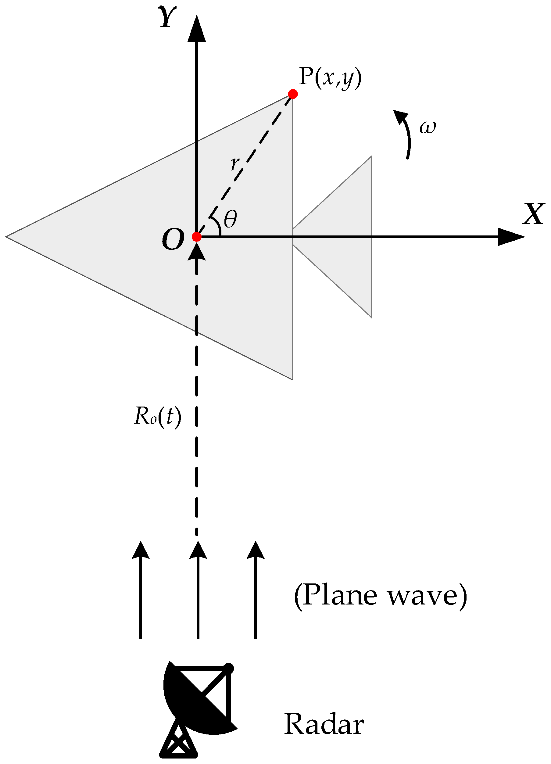
2.1. Signal Model

This section presents an exposition on the imaging geometry of ISAR and the derivation of the signal model attributed to a non-stationary moving target. Figure 1 shows the geometry for the ISAR imaging of a moving target. OXY is the target body coordinate system, and O is a reference point of the target. The target is presumed to be a model with P scatterers, and p is the pth scatterer with its coordinate of $\left(x_p,y_p\right)$.

In general, the ISAR system transmits wideband signals such as chirp signals and stepped frequency signals in order to achieve high range resolution [14,26]. Without a loss of generality, it is assumed that the ISAR system transmits a chirp signal as

$$s_t\left(\hat{t}\right)=\mathrm{rect}\left(\frac{\hat{t}}{T_p}\right)\exp \left\{\mathrm{j}2\pi \left(f_c\hat{t}+\frac{1}{2}\mu {\hat{t}}^2\right)\right\},$$

(1)

where $T_p$ is the pulse width, $\widehat{t}\in \left[-T_p/2,T_p/2\right]$ is the fast time, $f_c$ is the carrier frequency, $\mu$ is the chirp rate, and rect(·) is defined by

$$\mathrm{rect}\left(u\right)=\{\begin{array}{c}\begin{array}{cc}1& \left|u\right|\le 1/2\end{array}\\ \begin{array}{cc}0& \left|u\right|>1/2\end{array}\end{array}.$$

(2)

Assuming that N represents the number of pulses and $\Delta T$ denotes the pulse repetition interval, slow time $t$ can be denoted as $n\cdot \Delta T,n=1,2,\cdots ,N$. After demodulation, the received baseband signal can be expressed in terms of fast time $\widehat{t}$ and slow time $t$ as follows:

$$s_r(\widehat{t},t)={\displaystyle \sum }_{p=1}^P{\sigma }_p\mathrm{rect}\left(\frac{\widehat{t}-\frac{2R_p(t)}{c}}{T_p}\right)\exp \left\{\mathrm{j}\pi \mu {\left(\widehat{t}-\frac{2R_p(t)}{c}\right)}^2\right\}\exp \left\{-\mathrm{j}4\pi \frac{R_p(t)}{\lambda }\right\},$$

(3)

where ${\sigma }_p$ is the backscattering coefficient of the pth scatterer, $c$ is the speed of light, $\lambda$ is the wavelength, and $R_p(t)$ represents the pth scatterer’s range distance from the radar.

Range compression is performed to obtain the compressed signal of the received signal, as shown in (4):

$$s_c(\widehat{t},t)={\displaystyle \sum }_{p=1}^P{\sigma }_p^{\prime }\sin \mathrm{c}\left[B\left(\widehat{t}-\frac{2R_p(t)}{c}\right)\right]\exp \left\{-\mathrm{j}\frac{4\pi R_p(t)}{\lambda }\right\},$$

(4)

where $B$ is the bandwidth of the transmitted signal, and ${\sigma }_p^{\prime }$ is the amplitude of the pth scatterer after range compression.

In the far field, the electromagnetic wave incident of the observation target can be regarded as a plane wave. In this case, the instantaneous distance, $R_p\left(t\right)$, from the pth scatterer to the radar can be approximated as

$$R_p\left(t\right)\approx R_o\left(t\right)+r\sin \theta \left(t\right),$$

(5)

where $R_o\left(t\right)$ is the distance from reference point O to the radar, and $\left(r,\theta \left(t\right)\right)$ is the polar coordinate of the pth scatterer.

Let the initial polar angle of the pth scatterer be ${\theta }_0$, then

$$\{\begin{array}{c}{x}_p=r\cos {\theta }_0\\ y_p=r\sin {\theta }_0\end{array}.$$

(6)

In addition, $\theta \left(t\right)={\theta }_0+\Delta \theta \left(t\right)$ where $\Delta \theta \left(t\right)$ represents the rotation angle. Substituting $\theta \left(t\right)$ into (5) yields

$$\begin{array}{cc}\hfill R_p\left(t\right)& \approx R_o\left(t\right)+r\sin \left({\theta }_0+\Delta \theta \left(t\right)\right)\hfill \\ & =R_o\left(t\right)+y_p\cos \left(\Delta \theta \left(t\right)\right)+x_p\sin \left(\Delta \theta \left(t\right)\right)\hfill \end{array}.$$

(7)

Since the rotation angle $\Delta \theta \left(t\right)$ during the observation time is small enough [27], the following approximations are obtained [28]:

$$\{\begin{array}{l}\cos \left(\Delta \theta \left(t\right)\right)\approx 1\\ \sin \left(\Delta \theta \left(t\right)\right)\approx \Delta \theta \left(t\right)\end{array}.$$

(8)

Substituting (8) into (7) yields

$$R_p\left(t\right)=R_o\left(t\right)+y_p+x_p\Delta \theta \left(t\right).$$

(9)

According to (4) and (9), $s_c(\widehat{t},t)$ can be written as

$$s_c(\widehat{t},t)={\displaystyle \sum }_{p=1}^P{\sigma }_p^{″}\exp \left\{-\mathrm{j}\frac{4\pi \left[R_o\left(t\right)+y_p+x_p\Delta \theta \left(t\right)\right]}{\lambda }\right\},$$

(10)

where ${\sigma }_p^{″}$ is the pth scatterer’s coefficient. In the Doppler modulation phase, $R_o\left(t\right)$ is generated by translation motion, which will degrade the ISAR images and needs to be compensated for. It is assumed that the required compensation is already carried out by conventional methods [7,8,9]. In addition, the Taylor approximation of $\Delta \theta \left(t\right)$ is given in (11):

$$\Delta \theta \left(t\right)\approx {\omega }_{1}t+\frac{1}{2}{\omega }_2{t}^2,$$

(11)

where ${\omega }_1$ and ${\omega }_2$ represent the angular velocity and angular acceleration, respectively. As a result, (10) can be rewritten as

$$s_c(\widehat{t},t)={\displaystyle \sum }_{p=1}^P{\sigma }_p^{″}\exp \left\{-\mathrm{j}\frac{4\pi \left[y_p+x_p\left({\omega }_{1}t+\raisebox{1ex}{$1$}\!\left/ \!\raisebox{-1ex}{$2$}\right.{\omega }_2{t}^2\right)\right]}{\lambda }\right\}.$$

(12)

It is obvious that the target’s non-stationary motion destroys the linear phase of the compressed signal. The received signal can be thought of as a chirp signal with P components along slow time. For the pth component, its center frequency and chirp rate are $2x_p{\omega }_1/\lambda$ and $2x_p{\omega }_2/\lambda$, respectively. In this condition, only by realizing Doppler analyses at each slow time point can high-quality ISAR images be obtained.

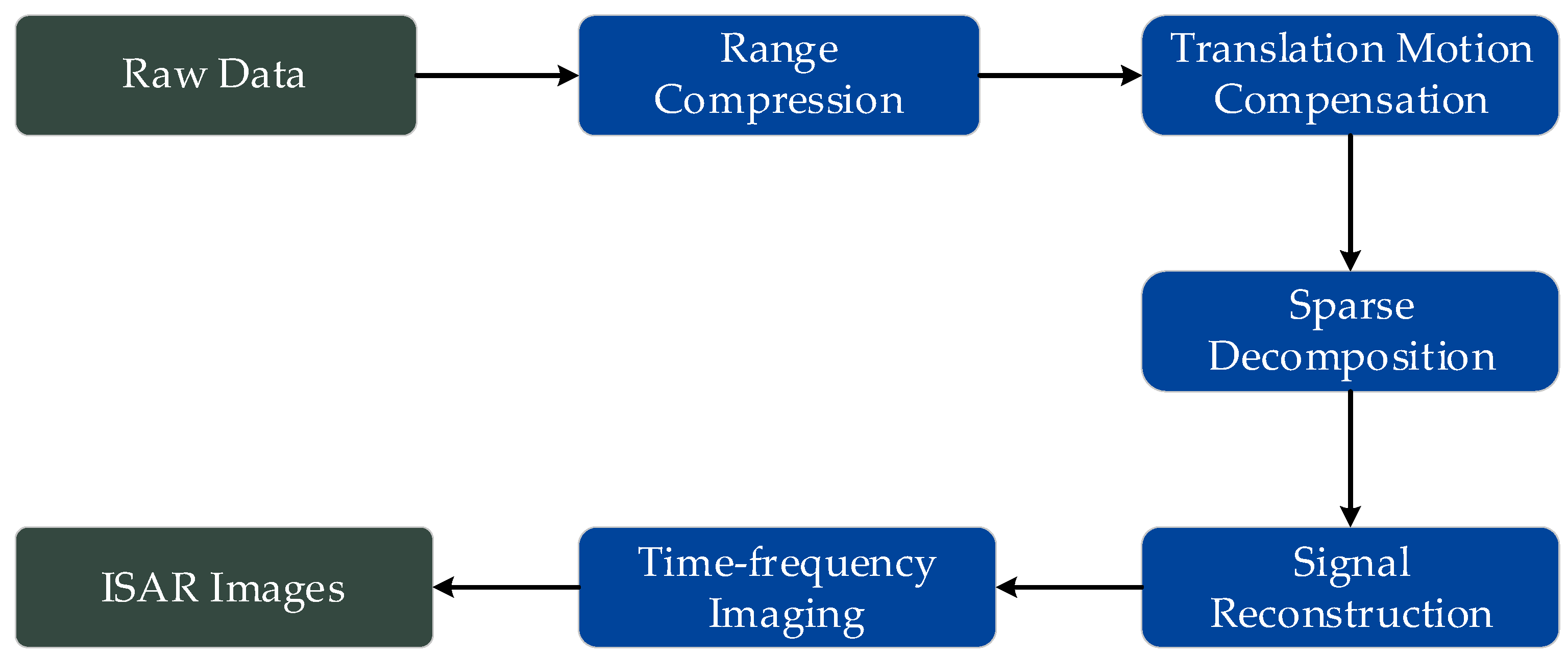
2.2. ISAR Imaging via Parameter Estimation and Sparse Decomposition

In this section, a non-searching ISAR imaging method for a non-stationary moving target is proposed. The received signals’ parameters are initially estimated with LVD. Subsequently, signal reconstruction is performed using sparse representation using a redundant dictionary. After that, the procedure of the proposed imaging method is given.

2.2.1. Parameter Estimation

As shown in (12), it is observed that the azimuth of the signal can be expressed as a chirp:

$$s_c(t)={\displaystyle \sum }_{p=1}^P{\sigma }_p^{″}\exp \left\{-\mathrm{j}\left({\phi }_p+2\pi f_{p}t+\pi {\mu }_p{t}^2\right)\right\},$$

(13)

where ${\phi }_p=4\pi y_p/\lambda$, $f_p=2x_p{\omega }_1/\lambda$, and ${\mu }_p=2x_p{\omega }_2/\mathsf{\lambda }$.

Accordingly, it is possible to estimate the center frequency and chirp rate using LVD [25], which has performed remarkably in chirp analyses without running a search [29,30,31]. A detailed solution will be presented in the following paragraphs.

The parametric symmetric instantaneous autocorrelation function (PSIAF) of $s_c(t)$ is defined as follows:

$$\begin{array}{cc}\hfill R_s& =s_c\left(t+\frac{\tau +a}{2}\right){s_c}^{*}\left(t-\frac{\tau +a}{2}\right)\hfill \\ & ={\displaystyle \sum _{p=1}^P{\left|{\sigma }_p^{″}\right|}^2\cdot \exp \left\{-\mathrm{j}2\pi f_p\left(\tau +a\right)-\mathrm{j}2\pi {\mu }_{p}t\left(\tau +a\right)\right\}}+R_{Cross-Terms}\hfill \end{array},$$

(14)

where $\tau$ is the time lag variable, $a$ is a constant, and $R_{Cross-Terms}$ represents the cross terms.

From (14), time variable $t$ is coupled to lag variable $\tau$. It is possible to construct virtual time variable $t_n=t\left(\tau +a\right)$. Replacing $t$ in (14) with $t_n$ yields

$$\overline{R_s}={\displaystyle \sum _{p=1}^P{\left|{\sigma }_p^{″}\right|}^2\exp \left\{\mathrm{j}2\pi f_p\left(\tau +a\right)+\mathrm{j}2\pi {\mu }_p{t}_n\right\}}+{\overline{R}}_{CrossTerms},$$

(15)

where ${\overline{R}}_{CrossTerms}$ represents the cross terms after the scaling transform.

The above expression is the decoupled PSIAF, for which a 2D-FFT is performed to obtain the LVD of $s_c(t)$, as shown in (16):

$$\begin{array}{cc}\hfill \mathrm{LVD}\left[s_c(t)\right]& ={\mathrm{FFT}}_{2D}\left[\overline{R_s}\right]\hfill \\ & ={\displaystyle \sum _{p=1}^P{\left|{\sigma }_p^{″}\right|}^2\delta \left(f-f_p\right)\delta \left(\mu -{\mu }_p\right)}+\mathrm{FT}{\overline{R}}_{CrossTerms}\hfill \end{array},$$

(16)

where $\mathrm{FT}{\overline{R}}_{CrossTerms}$ represents the cross terms after FFT.

According to Appendix A, the cross terms cannot accumulate coherently after the FFT and will slightly influence the result. Therefore, the LVD has an asymptotic linear property, as shown in (17).

$$\mathrm{LVD}\left[s_c(t)\right]\approx {\displaystyle \sum _{p=1}^P{\left|{\sigma }_p^{″}\right|}^2\delta \left(f-f_p\right)\delta \left(\mu -{\mu }_p\right)}.$$

(17)

From (17), the LVD of a multi-component chirp signal is equivalent to the sum of the LVD results of the components. This is presented in the center frequency chirp rate (CFCR) plane as a series of impulse functions. Parameter estimation results for each component are obtained by determining the coordinates of each extreme point.

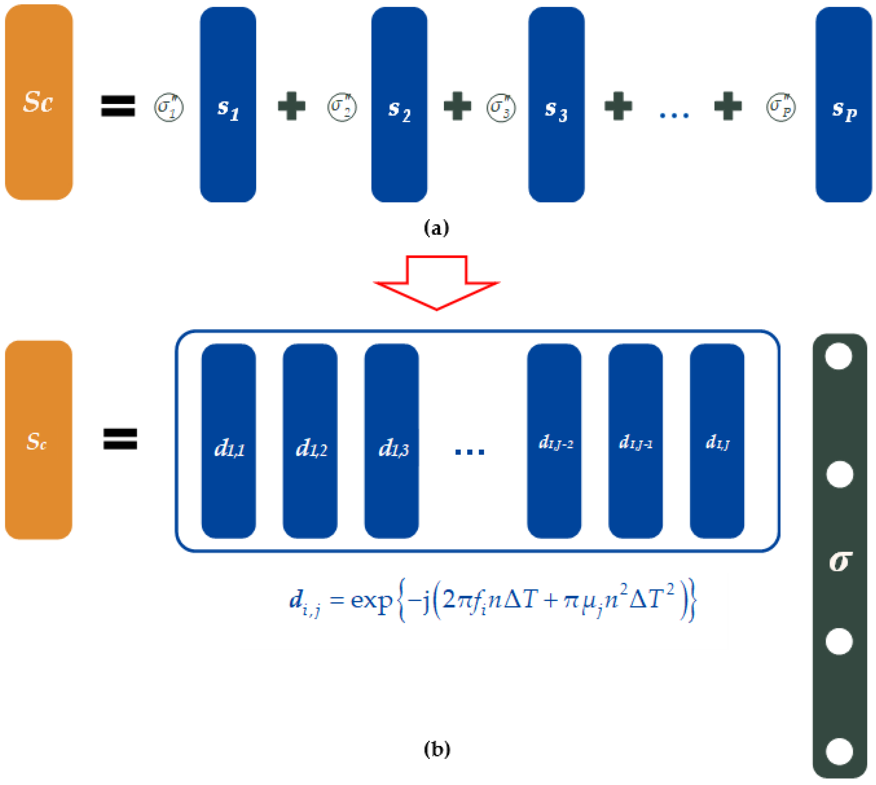
2.2.2. Sparse Decomposition

As (13) has shown, the azimuth of the received signal can be regarded as a multi-component chirp signal. The number of components corresponds to the number of scatterers belonging to the range cell. It is widely known that scatterers on the observation target are always limited and far smaller than the total sampling points, which means the data have inherent sparsity in the CFCR domain. Therefore, the theory of compressive sensing (CS) can be employed to reconstruct the sparse signal by solving an optimization problem [32,33]. The following is a detailed solution to the problem.

For convenience, (13) can be expressed in the following discrete form:

$$s_c\left(n\right)={\displaystyle \sum }_{p=1}^P{\sigma }_p^{″}{s}_p\left(n\right)\hspace{1em}1\le n\le N,$$

(18)

where $s_c$ is a N-dimensional vector representing the sampled signal, and the sample interval is $\Delta T$. The linear combination in (18) can be expressed as a matrix multiplication, as shown in Figure 2.

Figure 2a provides an intuitive representation of (18). It is clear that vector $s_c$ contains P components, and each of these components has a particular weight. Finally, vector $s_c$ arises via a weighted summation of the individual components. This operation adheres to the principles of matrix multiplication, which implies that the set of vectors $\left\{s_p\right\}$ and weight coefficients $\left\{{\mathsf{\sigma }}_p^{″}\right\}$ can be arranged as a matrix and a vector, respectively. Thus, (18) can be reformulated as follows:

$$s_c={\left[\begin{array}{cccc}{s}_1& s_1& \cdots & s_P\end{array}\right]}_{N\times P}{\left(\begin{array}{c}\begin{array}{c}{\mathsf{\sigma }}_1^{″}\\ {\mathsf{\sigma }}_2^{″}\end{array}\\ \begin{array}{c}⋮\\ {\mathsf{\sigma }}_P^{″}\end{array}\end{array}\right)}_{P\times 1}.$$

(19)

However, matrix $\left[\begin{array}{cccc}{s}_1& s_1& \cdots & s_P\end{array}\right]$ cannot be obtained due to the unknown parameters of the echoes. Fortunately, according to the previous derivation, all column vectors of this matrix represent chirp signals with various parameters. The matrix can be expanded into a “flat matrix” (called a chirp dictionary), yielding a dense distribution of chirp signal parameters. This operation ensures that the analyzed signal belongs to the space spanned by the chirp dictionary. At the same time, the dimension of the weight vector will also increase accordingly. In this way, the matrix multiplication’s form, which is depicted in Figure 2b, will emerge. As is evident, there are only a few column vectors that are contributing to the matrix multiplication, so the weight vector exclusively allocates a value at the corresponding positions, leaving all other positions zero.

Then, the chirp dictionary can be defined as

$$D={\left\{d_{1,1}\cdots d_{1,J}\cdots d_{I,1}\cdots d_{I,J}\right\}}_{N\times I\cdot J},$$

(20)

where $d_{i,j}=\exp \left\{-\mathrm{j}\left(2\pi f_{i}n\Delta T+\pi {\mu }_j{n}^2\Delta T^2\right)\right\}$, $1\le i\le I$, $1\le j\le J$. Furthermore, I and J are large enough that $D$ includes all signal components.

Therefore, the signal of the range cell can be rewritten in a condensed form as follows:

$$s_c=D \sigma +\epsilon ,$$

(21)

where $\sigma \in {ℂ}^{I\cdot J\times 1}$ is a sparse vector, and $\epsilon \in {ℂ}^{N\times 1}$ is the noise vector.

The goal is to obtain the solution of unknown vector $\sigma$ based on defined dictionary matrix $D$ and signal vector $s_c$. The solution can be acquired by solving an optimization problem as follows:

$$\langle \widehat{\sigma }\rangle =\arg \underset{\sigma }{\min } {\Vert \sigma \Vert }_0\hspace{1em}\mathrm{s}.\mathrm{t}.\hspace{1em}{\Vert s_c-D \sigma \Vert }_2\le {\Vert \epsilon \Vert }_2,$$

(22)

where ${\Vert \sigma \Vert }_0$ represents the number of nonzero components in $\sigma$, and ${\Vert \epsilon \Vert }_2$ is the noise level that can be estimated by the noise range cells.

This l₀-norm optimization belongs to NP-hard problems and can be handled by some methods [34,35,36,37]. However, due to the dictionaries’ high dimensionality, considerable computational expenses and memory consumption exist. In order to address this issue, an effective reconstruction algorithm combined with LVD has been developed for the optimization problem.

The proposed algorithm accepts signal vector $s_c$ and required sparsity K and outputs parameter estimates, such as ${\widehat{\sigma }}_p^{″}$, ${\widehat{f}}_p$, and ${\widehat{\mu }}_p$, for each signal component. As shown in Figure 3, the algorithm includes the following steps:

(1) Let the iteration count variable be $t=1$, which is the set of signal vectors determined in the tth iteration ${\Phi }_t=\varnothing$, and the residual signal of the tth iteration is $r_t=s_c$;

(2) Calculate the LVD of $r_t$ and subsequently select the signal vectors corresponding to the first K large extreme value points to construct set $A_{tN\times K}$. At the same time, their center frequencies and chirp rates are saved as ${\widehat{f}}_{K\times 1}$ and ${\widehat{\mu }}_{K\times 1}$, respectively;

(3) Use the union of $A_t$ and ${\Phi }_t$ to perform a least squares regression for $s_c$. Then, screen the top t vectors with the highest expression coefficients and save them as ${\left[e_1,e_2,\cdots ,e_t\right]}_{N\times t}$. In addition, these coefficients are preserved as ${\widehat{\sigma }}_t={\left({\widehat{\sigma }}_1,{\widehat{\sigma }}_2,\cdots ,{\widehat{\sigma }}_t\right)}^T$, and $\widehat{f}$ and $\widehat{\mu }$ are also adjusted to ${\widehat{f}}_t={\left({\widehat{f}}_1,{\widehat{f}}_2,\cdots ,{\widehat{f}}_t\right)}^T$ and ${\widehat{\mu }}_t={\left({\widehat{\mu }}_1,{\widehat{\mu }}_2,\cdots ,{\widehat{\mu }}_t\right)}^T$, respectively;

(4) Perform the following parameter updates:

$$\{\begin{array}{l}{\Phi }_t=\left[e_1,e_2,\cdots ,e_t\right]\hfill \\ r_t={\mathrm{Proj}}_{{\Phi }_t}^{\perp }{s}_c=\left[I-{\Phi }_t{\left({{\Phi }_t}^H{\Phi }_t\right)}^{-1}{{\Phi }_t}^H\right]s_c\hfill \\ t=t+1\hfill \end{array},$$

(23)

where I is the unit matrix, and ${{\Phi }_t}^H$ represents the conjugate transpose matrix of ${\Phi }_t$;

(5) Determine when to terminate the iteration: if $t>K$ or ${\Vert r_t\Vert }^2\le {\Vert \epsilon \Vert }^2$, jump out of the loop and stop the iteration; otherwise, jump to step (2) and continue the iteration.

The algorithm takes advantage of the excellent time–frequency aggregation of LVD to accurately estimate the input signal’s center frequency and chirp rate and performs preliminary vector screening. Then, the vectors of this iteration are determined by the least squares (LS) method. On the one hand, two-step screening can increase the precision of parameter estimation, and on the other hand, it can give the algorithm some fault tolerance. In the third step, old and new vectors are merged and examined as a whole, which implies that the vectors selected in the preceding iterations are not kept indefinitely, and if an incorrect vector was chosen in the last iteration, then it will be eliminated in the ensuing iteration. Finally, the input signal vector is projected into the orthogonal complement space of the determined vectors set to remove the selected signal vectors, thereby yielding the residual signal.

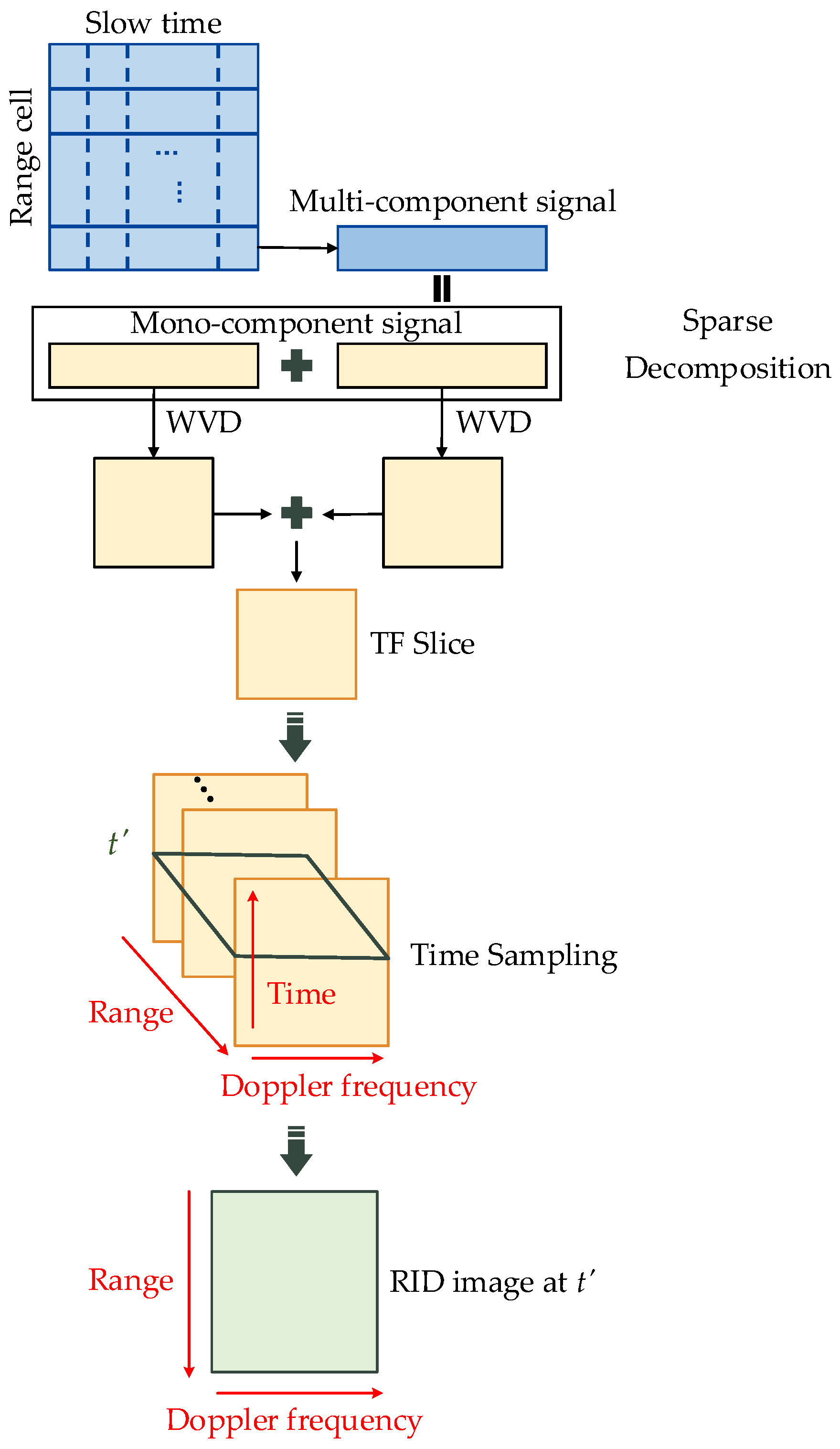
2.2.3. Signal Reconstruction and ISAR Imaging

The previous subsection elucidates the process of decomposing the echo signal with the proposed method in detail. At the termination of the iteration (assume a total of P iterations), amplitude ${\widehat{\sigma }}_P$, center frequency ${\widehat{f}}_P$, and the chirp rate ${\widehat{\mu }}_P$ of individual components contained in the input signal can be determined, which can be provided as follows:

$${\widehat{\sigma }}_P={\left({\widehat{\sigma }}_1,{\widehat{\sigma }}_2,\cdots ,{\widehat{\sigma }}_P\right)}_{P\times 1}^T,$$

(24)

$${\widehat{f}}_P={\left({\widehat{f}}_1,{\widehat{f}}_2,\cdots ,{\widehat{f}}_P\right)}_{P\times 1}^T,$$

(25)

$${\widehat{\mu }}_P={\left({\widehat{\mu }}_1,{\widehat{\mu }}_2,\cdots ,{\widehat{\mu }}_P\right)}_{P\times 1}^T.$$

(26)

By utilizing these data, input signal vector $s_c$ can be readily reconstructed as follows:

$${\widehat{s}}_c={\displaystyle \sum _{p=1}^P{\widehat{s}}_p},$$

(27)

$${\widehat{s}}_p={\widehat{\sigma }}_p\cdot \exp \left\{-\mathrm{j}\left(2\pi {\widehat{f}}_{p}n\Delta T+\pi {\widehat{\mu }}_p{n}^2\Delta T^2\right)\right\}\hspace{1em}1\le n\le N.$$

(28)

Then, adaptive joint time–frequency imaging techniques shown in Figure 4 are used to produce high-quality images of the non-stationary moving target with the reconstructed data [38]. To avoid the cross-term interface, the individual component present in the reconstructed signal, ${\widehat{s}}_c$, is subjected to separate WVD processing. Subsequently, the time–frequency (TF) slice of the range cell is acquired by summing up the WVD of all components.

$$TF={\displaystyle \sum _{p=1}^{P}WVD\left\{{\widehat{s}}_p\right\}}.$$

(29)

Naturally, the TF slices produced by Equation (29) are devoid of any cross terms. After performing the same operation for the entire range cells, the third-order tensor (time × range × Doppler frequency) becomes available to yield a series of RID images of the target via time sampling.

Ultimately, the comprehensive processing flowchart depicted in Figure 5 can be attained. Initially, range compression processing must be executed on the raw data received from the radar. Range compression is usually achieved by a matched filter, and it can convert echo signals from the frequency space to the range space, which indicates the range of each scattering point. Subsequently, translation motion compensation (TMC) must be performed. The target’s motion can be decomposed into translation and rotation. Translation motion provides no assistance for imaging and needs to be compensated for as much as possible. TMC always includes two steps: range alignment and phase adjustment. By implementing TMC, the negative effects of the target translation on both the range envelope and signal phase can be compensated for, thereby enabling the treatment of the target as a non-stationary revolving object. Based on this, the sparse decomposition algorithm proposed in this article can be employed to process each range cell signal. After that, several mono-component signals can be employed to reconstruct the original signal, after which the proposed sparse decomposition and time–frequency imaging technique can be utilized to achieve high-resolution ISAR images of the target that are free of any cross-term interference.

3. Results

In this section, extensive simulation experiments were conducted with LVD to verify the robustness of the technique and explore the estimation performance of weak components in the signals. In addition, simulated and measured data are treated with the proposed ISAR imaging algorithm, and the experimental results reveal its efficacy. For the purposes of comparison, the results were compared with the classical RD [12] method, the CLEAN method [23], and two RID methods that comprise TF analysis methods: STFT [20] and smoothed pseudo-Wigner–Ville Distribution (SPWVD) [39].

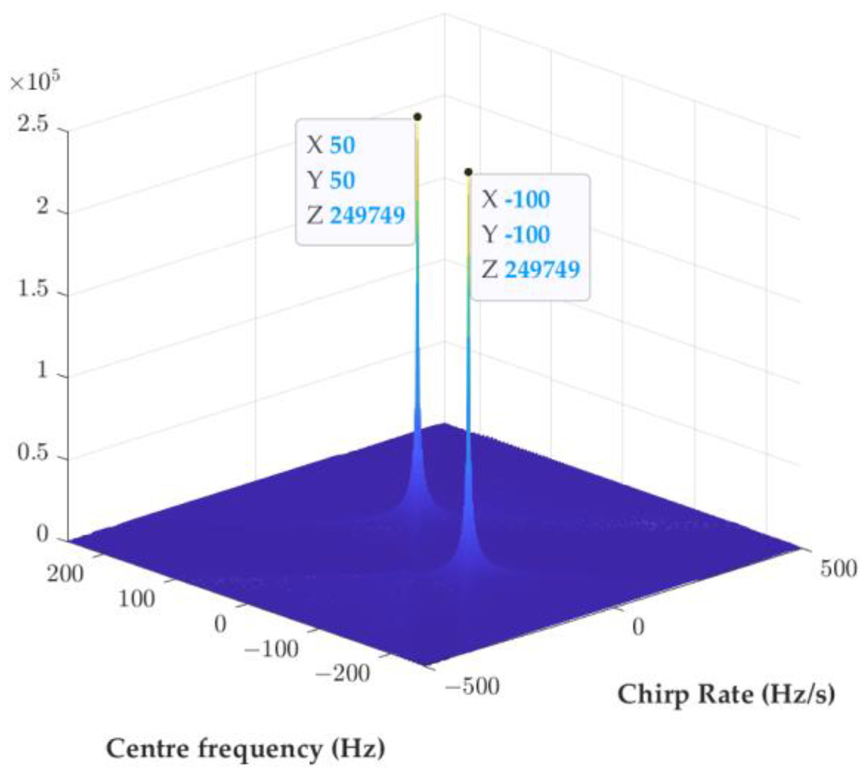
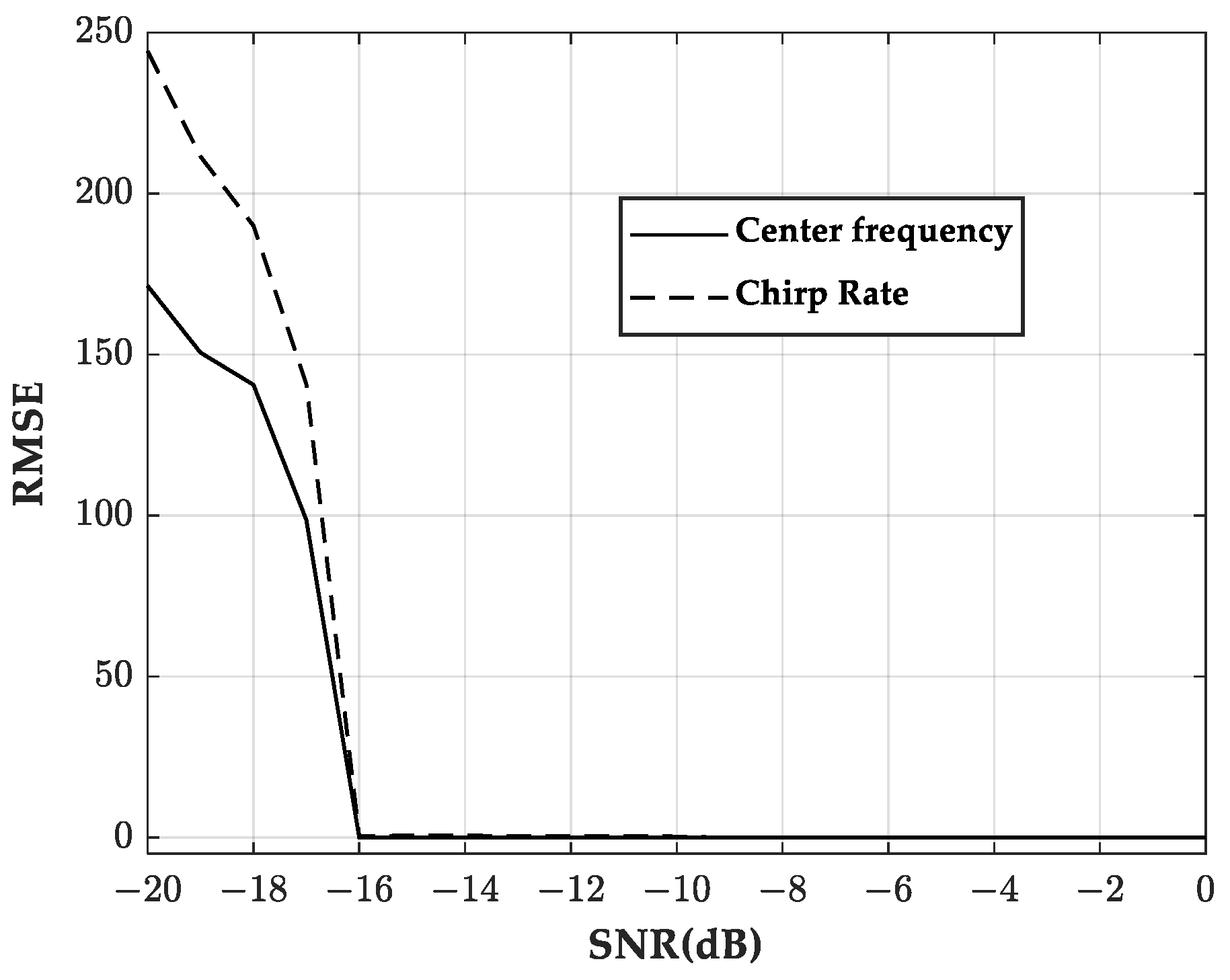
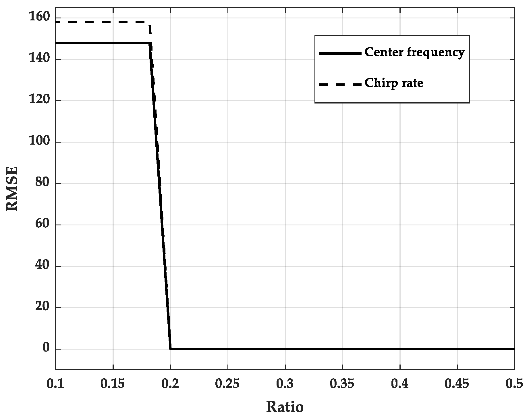
3.1. LVD Estimation Results

A signal containing two components is generated to verify the robustness of LVD. The two components have the same amplitude, and their center frequencies and chirp rates are (−100 Hz and −100 Hz/s) and (50 Hz and 50 Hz/s), respectively. The LVD results for this signal under ideal conditions are given in Figure 6. LVD accurately obtains the parameters of both components, and there are few cross-terms in the CFCR plane.

Extensive simulations are delivered to emphasize the accuracy and robustness of the method. One thousand Monte Carlo simulations were performed for each SNR value, where the SNR spans from −20 to 0 dB with a step of 1 dB. The graphical representation of the relationship existing between the root mean square error (RMSE) of the estimation and SNR is provided in Figure 7. The results demonstrate that the LVD method exhibits a notable level of robustness, thereby enabling the precise estimation of signal parameters even at a relatively low SNR of −16 dB.

Subsequent experiments were conducted to scrutinize the performance of the estimation of the weak components present in the signal. Based on the aforementioned signals, a new component was introduced, featuring a center frequency of −40 Hz and a chirp rate of −40 Hz/s. In the course of the experiment, the new component’s amplitude is steadily attenuated from 50% to 10% of the other components to investigate the estimation performance for the weak component. Figure 8 illustrates the RMSE outcomes obtained by LVD for the weak component. The findings suggest that the signal parameters can be accurately estimated by the LVD method when the amplitude of the weak component amounts to 20% of the strong one. Frankly speaking, the performance is adequate to satisfy the requirements of the proposed method in this article, given that dominant components will gradually be eliminated during the iterative process. As a result, previously weak components will become relatively stronger in subsequent iterations, thereby facilitating their accurate detection.

3.2. Simulated Data Processing Results

The simulated data used in this paper are based on the MiG-25 fighter scatter point model [40], which is provided by Victor C. Chen from the United States Naval Research Laboratory. It contains 120 points, and the backscattering coefficients of all points are 1 for the sake of simplicity, as shown in Figure 9. For convenient analysis, we enlarged the size of the model, and it possesses a wingspan of 32.00 m and a length of 54.00 m. By virtue of the massive points, the model can emulate classic aircraft targets. The ISAR system transmits chirp signals, and some system parameters are shown in

Table 1. ISAR system parameters for the simulated data.

Parameters	Values
Carrier frequency	10 GHz
Signal bandwidth	100 MHz
Pulse repetition frequency	100 Hz
Range samples	80
Azimuth samples	256

.

During the simulation, the target moves non-stationarily, and after the ideal TMC, the target still has an angular velocity of 0.01 $\mathrm{rad}/\mathrm{s}$ and an angular acceleration of 0.03 ${\mathrm{rad}/\mathrm{s}}^2$. Moreover, the SNR of the simulation data is 10 dB.

Figure 10 shows the range compression profiles after TMC. The slow time signal of each range cell can be considered to be a multi-component signal. Due to the fact that there are 12 points at most within 1 range cell in the scatterer point model, sparsity K is taken to be 15 for the experiment.

Figure 11a shows the distribution of the number of scatterers with the range cell obtained by our sparse recovery algorithm. From the distribution, it can be observed that there are more scatterers in the middle and sides of the target and fewer scatterers in the rest of the target. This conclusion coincides with the fact that the MiG-25 fighter model has more scatterers at the fuselage’s central axis and the ends of the wings. Figure 11b presents the reconstructed range profiles by applying the proposed sparse decomposition algorithm. After sparse decomposition and signal reconstruction, not only can the intrinsic structure of the signals be well characterized but the purpose of noise suppression can also be achieved.

Figure 12 shows the ISAR imaging results obtained by different methods. The blurred and incorrect areas in the results are marked by white circles. The non-stationary movement of the target leads to a time-varying Doppler frequency that will defocus the ISAR image. The results by RD illustrate this fact well, as shown in Figure 12a. The energy of each scatterer is not focused as a point but disperses within several Doppler cells, and it results in image degradation. It is obvious that the introduction of the TF analysis can significantly improve image quality, as shown in Figure 12. However, STFT and SPWVD are limited by the low TF resolution due to the side effects of windowing, as demonstrated in Figure 12b,c. The scatterers on the tail of the fighter in these two images are blended in a completely indistinguishable way and so are the scattering points in the front area. Figure 12d presents the ISAR image acquired via the utilization of the CLEAN technique. Despite the deployment of a search interval and step size, limitations in matching these parameters to the actual situation result in suboptimal image quality, which is characterized by the emergence of erroneous scattering points. Finally, Figure 12e shows a well-focused image created by the proposed method. Due to the signal reconstruction, the image is generated via mono-component signals, making the results free of cross-term interference, and they exhibit high resolution. The proposed method produces high resolution in the Doppler dimension, allowing the clear distinguishing of each scatterer, which corresponds almost exactly to the original scatterer point model.

3.3. Measured Data Processing Results

The observation target for the measured data used in this paper is the Yak-42 aircraft, [23] which is 36.38 meters long and 34.88 meters wide, as shown in Figure 13. The data were recorded by a C-band ISAR system. The radar transmitted chirp signals, and the received signals were de-chirped and I/Q sampled. Necessary TMC measures have been implemented to compensate for translation motion. The ISAR system parameters are exhibited in

Table 2. ISAR system parameters for the measured data.

Parameters	Values
Carrier frequency	5.52 GHz
Signal bandwidth	400 MHz
Pulse repetition frequency	100 Hz
Range samples	256
Azimuth samples	256

. In addition, the SNR of the measured data is 10 dB.

These measured data were processed using the proposed method with K = 10, and the reconstruction results are illustrated in Figure 14. The range compression data have been processed by TMC, as shown in Figure 14a. The sparse reconstruction algorithm proposed in this article is employed to process the range profiles, and Figure 14b highlights the number of scatterers for each range cell. The output results indicate that the scattering points of the target are mainly concentrated in the 119th to 138th range cells. This conclusion is consistent with the actual situation. After sparse decomposition and signal reconstruction, reconstructed range profile data can be obtained, which are depicted in Figure 14c.

The proposed time–frequency imaging method is executed subsequently, and the ISAR image shown in Figure 15e can be obtained. For comparison purposes, alternative methods are also employed to process the same data, and the results are also listed in Figure 15. As observed, the image by the proposed method has more structural information as well as higher resolution. This is because the sparse decomposition and signal reconstruction algorithm proposed in this paper analyzes the signal in terms of a single scatterer. This is the reason why it can remove cross-term interference. It eliminates most noise, clutter, and some weak scatterers, while only the main scatterers are preserved. The visible “point feature” in the images of our method highlights the strong scattering points on the target, which is meaningful for feature extraction and target recognition. Conversely, other methods weaken the scattering point information of the target, which can be observed at the tail and wing part of the aircraft, as shown in Figure 15a,b. The improved focus of the images generated by SPWVD and CLEAN is accompanied by a significant reduction in the number of weak scatterings, leading to image distortion. This phenomenon may adversely affect the interpretation and analysis of the image data. Even in the area of weak scattering at the front of the aircraft, the scatterers can also be identified by using the proposed approach.

4. Discussion

To evaluate the performance of different methods objectively, image entropy is used as a metric to quantify their imaging performance. For an ISAR image $G\left(m,n\right)$, its image entropy, E, can be calculated by the following (30):

$$E={\displaystyle \sum _{m=1}^M{\displaystyle \sum _{n=1}^{\mathrm{N}}\frac{{\left|G\left(m,n\right)\right|}^2}{S}\ln \frac{S}{{\left|G\left(m,n\right)\right|}^2}}},$$

(30)

where $S={\displaystyle \sum _{m=1}^M{\displaystyle \sum _{n=1}^{\mathrm{N}}{\left|G\left(m,n\right)\right|}^2}}$, and M and N are the numbers of samples in the range direction and the cross-range direction, respectively [41].

The entropy calculation results of different ISAR images in previous experiments are provided in Figure 16. It is apparent from this figure that the entropy of the image generated by the proposed method is the lowest, while the others are noticeably higher. Their entropy differs by almost 25%. The exceptional imaging performance of the method can be inferred from this fact.

To investigate the focusing performance of different methods, the signal waveforms of the 21st range cell of MiG-25 and the 160th range cell of Yak-42 are drawn in Figure 17. An inspection of the pulse width in this figure reveals that the proposed method performs outstandingly, both for the widening of the main lobe and for the suppression of the side lobe. Because of the non-stationary movement, the RD method is unsurprisingly the worst performer, with scatterers barely being in focus. The effectiveness of the CLEAN method is affected by the accuracy of the estimation and is further subject to significant fluctuations in terms of its focusing performance. The other two methods are better than RD, but their global performance is still inferior to the proposed method.

Evidently, the proposed ISAR imaging method has the lowest entropy, the best focusing performance, and the highest quality image. The simulation results announce the sophistication of the proposed method. According to the experimental results, the proposed method has obvious advantages both in terms of image entropy and time–frequency resolution. This is attributed to our decomposition of multi-component signals into mono-component signals and precise parameter estimation, which can avoid cross terms from the origin and also eliminate side effects caused by windowing, maintaining the high resolution of the time–frequency analysis method.

5. Conclusions

This paper addresses the issue of parameter estimation and signal reconstruction in the ISAR imaging of non-stationary moving targets. Traditional RD methods often result in blurred images due to the non-stationary motion of the target. TF analysis methods are typically limited by the trade-off between time–frequency resolution and cross-term interference. Against this background, a novel ISAR imaging method based on parameter estimation and sparsity recovery is proposed in this article. By combining LVD with the proposed sparse recovery algorithm, the received multi-component signals are resolved accurately into the sum of mono-component signals by exploiting the sparsity of the data in the CFCR domain. The signal reconstruction allows us to map the intrinsic structural properties of the received signals. Then, the proposed adaptive joint time–frequency imaging method is employed to acquire high-quality ISAR images of the target. The proposed method has the advantages of being cross-term-free and exhibiting high resolution, providing it with excellent imaging performance. The experimental results of both simulated and measured data demonstrate the effectiveness of the proposed approach.

References

1. Cooke, T.; Martorella, M.; Haywood, B.; Gibbins, D. Use of 3D ship scatterer models from ISAR image sequences for target recognition. Digit. Signal Process. 2006, 5, 523–532. [Google Scholar] [CrossRef]
2. Lee, S.J.; Lee, M.J.; Kim, K.T.; Bae, J.H. Classification of ISAR Images Using Variable Cross-Range Resolutions. IEEE Trans. Aerosp. Electron. Syst. 2018, 5, 2291–2303. [Google Scholar] [CrossRef]
3. Li, W.; Yuan, Y.; Zhang, Y.; Luo, Y. Unblurring ISAR Imaging for Maneuvering Target Based on UFGAN. Remote Sens. 2022, 14, 5270. [Google Scholar] [CrossRef]
4. Ozdemir, C. Inverse Synthetic Aperture Radar Imaging with MATLAB Algorithms, 2nd ed.; John Wiley and Sons, Inc.: Hoboken, NJ, USA, 2021. [Google Scholar]
5. Cumming, I.G.; Wong, F.H. Digital Processing of Synthetic Aperture Radar Data Algorithms and Implementation; Artech House Publishers: Norwood, Hong Kong, 2005. [Google Scholar]
6. Berizzi, F.; Mese, E.D.; Diani, M.; Martorella, M. High-resolution ISAR imaging of maneuvering targets by means of the range instantaneous Doppler technique: Modeling and performance analysis. IEEE Trans. Image Process. 2001, 12, 1880–1890. [Google Scholar] [CrossRef]
7. Li, D.; Zhan, M.; Liu, H.; Liao, Y.; Liao, G. A Robust Translational Motion Compensation Method for ISAR Imaging Based on Keystone Transform and Fractional Fourier Transform Under Low SNR Environment. IEEE Trans. Aerosp. Electron. Syst. 2017, 53, 2140–2156. [Google Scholar] [CrossRef]
8. Ustun, D.; Toktas, A. Translational Motion Compensation for ISAR Images through a Multicriteria Decision Using Surrogate-Based Optimization. IEEE Trans. Geosci. Remote Sens. 2020, 58, 4365–4374. [Google Scholar] [CrossRef]
9. Kim, J.; Kim, S.; Cho, H.; Song, W.; Yu, J. Fast ISAR motion compensation using improved stage-by-stage approaching algorithm. J. Electromagn. Waves Appl. 2021, 12, 1587–1600. [Google Scholar] [CrossRef]
10. Liu, F.; Huang, D.; Guo, X.; Feng, C. Noise-Robust ISAR Translational Motion Compensation via HLPT-GSCFT. Remote Sens. 2022, 14, 6201. [Google Scholar] [CrossRef]
11. Yang, S.; Li, S.; Jia, X.; Cai, Y.; Liu, Y. An Efficient Translational Motion Compensation Approach for ISAR Imaging of Rapidly Spinning Targets. Remote Sens. 2022, 14, 2208. [Google Scholar] [CrossRef]
12. Jack, L.W. Range-Doppler Imaging of Rotating Objects. IEEE Trans. Aerosp. Electron. Syst. 1980, 1, 23–52. [Google Scholar] [CrossRef]
13. Jia, X.; Song, H.; He, W. A Novel Method for Refocusing Moving Ships in SAR Images via ISAR Technique. Remote Sens. 2021, 13, 2738. [Google Scholar] [CrossRef]
14. He, X.; Tong, N.; Hu, X.; Feng, W. High-resolution ISAR imaging of fast rotating targets based on pattern-coupled Bayesian strategy for multiple measurement vectors. Digit. Signal Process. 2019, 93, 151–159. [Google Scholar] [CrossRef]
15. Zhang, Y.; Xing, M. Cross-range scaling for non-uniformly rotating targets by sharpness maximization. Digit. Signal Process. 2019, 86, 29–35. [Google Scholar] [CrossRef]
16. Yang, Z.; Li, D.; Tan, X.; Liu, H.; Liu, Y.; Liao, G. ISAR Imaging for Maneuvering Targets with Complex Motion Based on Generalized Radon-Fourier Transform and Gradient-Based Descent under Low SNR. Remote Sens. 2021, 13, 2198. [Google Scholar] [CrossRef]
17. Li, X.; Kong, L.; Cui, G.; Yi, W.; Yang, Y. ISAR imaging of maneuvering target with complex motions based on ACCF–LVD. Digit. Signal Process. 2015, 46, 191–200. [Google Scholar] [CrossRef]
18. Zhan, M.; Huang, P.; Liu, X.; Liao, G.; Zhang, Z.; Wang, Z.; Fan, H. An ISAR imaging and cross-range scaling method based on phase difference and improved axis rotation transform. Digit. Signal Process. 2020, 104, 102798. [Google Scholar] [CrossRef]
19. Wang, Y.; Zhao, B.; Kang, J. Asymptotic Statistical Performance of Local Polynomial Wigner Distribution for the Parameters Estimation of Cubic-Phase Signal with Application in ISAR Imaging of Ship Target. IEEE J. Sel. Top. Appl. Earth Obs. Remote Sens. 2015, 8, 1087–1098. [Google Scholar] [CrossRef]
20. Wang, Y.; Lin, Y. ISAR Imaging of Non-Uniformly Rotating Target via Range-Instantaneous-Doppler-Derivatives Algorithm. IEEE J. Sel. Top. Appl. Earth Obs. Remote Sens. 2014, 7, 167–176. [Google Scholar] [CrossRef]
21. Bao, Z.; Sun, C.; Xing, M. Time-frequency approaches to ISAR imaging of maneuvering targets and their limitations. IEEE Trans. Aerosp. Electron. Syst. 2001, 37, 1091–1099. [Google Scholar] [CrossRef]
22. Stankovic, L. A method for time-frequency analysis. IEEE Trans. Signal Process. 1994, 42, 225–229. [Google Scholar] [CrossRef]
23. Zhang, L.; Duan, J.; Qiao, Z.J.; Xing, M.D.; Bao, Z. Phase adjustment and isar imaging of maneuvering targets with sparse apertures. IEEE Trans. Aerosp. Electron. Syst. 2014, 50, 1955–1973. [Google Scholar] [CrossRef]
24. Liu, F.; Huang, D.; Guo, X.; Feng, C. Unambiguous ISAR Imaging Method for Complex Maneuvering Group Targets. Remote Sens. 2022, 14, 2554. [Google Scholar] [CrossRef]
25. Lv, X.; Bi, G.; Wan, C.; Xing, M. Lv’s Distribution: Principle, Implementation, Properties, and Performance. IEEE Trans. Signal Process. 2011, 59, 3576–3591. [Google Scholar] [CrossRef]
26. Yang, T.; Shi, H.; Guo, J.; Qiao, Z. Orbital-angular-momentum-based super-resolution ISAR imaging for maneuvering targets: Modeling and performance analysis. Digit. Signal Process. 2021, 117, 103197. [Google Scholar] [CrossRef]
27. Zhu, D.; Ling, W.; Yu, Y.; Tao, Q.; Zhu, Z. Robust ISAR Range Alignment via Minimizing the Entropy of the Average Range Profile. IEEE Geosci. Remote Sens. Lett. 2009, 6, 204–208. [Google Scholar] [CrossRef]
28. Vehmas, R.; Jylha, J.; Vaila, M.; Vihonen, J.; Visa, A. Data-Driven Motion Compensation Techniques for Noncooperative ISAR Imaging. IEEE Trans. Aerosp. Electron. Syst. 2018, 54, 295–314. [Google Scholar] [CrossRef]
29. Luo, S.; Bi, G.; Lv, X.; Hu, F. Performance analysis on Lv distribution and its applications. Digit. Signal Process. 2012, 23, 797–807. [Google Scholar] [CrossRef]
30. Yu, W.; Su, W.; Hong, G. Ground moving target motion parameter estimation using Radon modified Lv’s distribution. Digit. Signal Process. 2017, 69, 212–223. [Google Scholar] [CrossRef]
31. Zhao, Y.; Han, S.; Yang, J.; Zhang, L.; Xu, H.; Wang, J. A Novel Approach of Slope Detection Combined with Lv’s Distribution for Airborne SAR Imagery of Fast Moving Targets. Remote Sens. 2018, 10, 764. [Google Scholar] [CrossRef]
32. Donoho, D.L. Compressed Sensing. IEEE Trans. Inf. Theory 2006, 52, 1289–1306. [Google Scholar] [CrossRef]
33. Candes, E.J.; Wakin, M.B. An Introduction to Compressive Sampling. IEEE Signal Process. Mag. 2008, 25, 21–30. [Google Scholar] [CrossRef]
34. Hashempour, H.R.; Masnadi-Shirazi, M.A. Inverse synthetic aperture radar phase adjustment and cross-range scaling based on sparsity. Digit. Signal Process. 2017, 68, 93–101. [Google Scholar] [CrossRef]
35. Chan, H.L.; Yeo, T.S. Noniterative quality phase-gradient autofocus (QPGA) algorithm for spotlight SAR imagery. IEEE Trans. Geosci. Remote Sens. 1998, 36, 1531–1539. [Google Scholar] [CrossRef]
36. Zhang, L.; Xing, M.; Qiu, C.W.; Li, J.; Sheng, J.; Li, Y.; Bao, Z. Resolution Enhancement for Inversed Synthetic Aperture Radar Imaging under Low SNR via Improved Compressive Sensing. IEEE Trans. Geosci. Remote Sens. 2010, 48, 3824–3838. [Google Scholar] [CrossRef]
37. Mohimani, H.; Babaie-Zadeh, M.; Jutten, C. A Fast Approach for Overcomplete Sparse Decomposition Based on Smoothed L-0 Norm. IEEE Trans. Signal Process. 2009, 57, 289–301. [Google Scholar] [CrossRef]
38. Chen, V.C.; Ling, H. Joint time-frequency analysis for radar signal and image processing. IEEE Signal Process. Mag. 1999, 16, 81–93. [Google Scholar] [CrossRef]
39. Qian, S.; Chen, D. Joint time-frequency analysis. IEEE Signal Process. Mag. 1999, 16, 52–67. [Google Scholar] [CrossRef]
40. Chen, V.C.; Martorella, M. Inverse Synthetic Aperture Radar Imaging; National Defense Industry Press: Beijing, China, 2020. [Google Scholar]
41. Sheng, J.; Xing, M.; Zhang, L.; Mehmood, M.Q.; Yang, L. ISAR Cross-Range Scaling by Using Sharpness Maximization. IEEE Geosci. Remote Sens. Lett. 2015, 12, 165–169. [Google Scholar] [CrossRef]
Figure 1. ISAR imaging geometry of a moving target.
Remotesensing 15 02368 g001
Figure 2. Vector form is represented in a matrix multiplication form. (a) Linear combination of vectors. (b) Matrix multiplication form.
Remotesensing 15 02368 g002
Figure 3. Flowchart of the proposed sparse decomposition algorithm.
Remotesensing 15 02368 g003
Figure 4. Diagram of sparse decomposition and adaptive joint time–frequency imaging techniques.
Remotesensing 15 02368 g004
Figure 5. Flowchart of the proposed ISAR imaging method based on parameter estimation and sparse decomposition.
Remotesensing 15 02368 g005
Figure 6. LVD results of a twocomponent signal without noise.
Remotesensing 15 02368 g006
Figure 7. RMSE with respect to SNR.
Remotesensing 15 02368 g007
Figure 8. RMSE with respect to the amplitude ratio.
Remotesensing 15 02368 g008
Figure 9. MiG25 fighter scatterer point model.
Remotesensing 15 02368 g009
Figure 10. Range compression profiles after TMC.
Remotesensing 15 02368 g010
Figure 11. Sparse decomposition and signal reconstruction results. (a) Distribution of the number of scatterers for each range cell. (b) Reconstructed results of the proposed signal reconstruction algorithm.
Remotesensing 15 02368 g011
Figure 12. ISAR imaging results of MiG-25. (a) Results by the RD method. (b) Result by the RID method with STFT. (c) Results by the RID method with SPWVD. (d) Results by the CLEAN method. (e) Results by the proposed imaging method.
Remotesensing 15 02368 g012
Figure 13. Yak-42 aircraft.
Remotesensing 15 02368 g013
Figure 14. Sparse decomposition and signal reconstruction results. (a) Range compression profiles after TMC. (b) Distribution of the number of scatterers for each range cell. (c) Reconstructed results of the proposed signal reconstruction algorithm.
Remotesensing 15 02368 g014
Figure 15. ISAR imaging results of Yak-42. (a) Results from the RD method. (b) Results from the RID method with STFT. (c) Results from the RID method with SPWVD. (d) Results from the CLEAN method. (e) Results from the proposed imaging method.
Remotesensing 15 02368 g015
Figure 16. Entropy of different imaging methods.
Remotesensing 15 02368 g016
Figure 17. Two range cells of different imaging methods. (a) The 21st range cell of MiG-25. (b) Results after zooming in (a). (c) The 160th range cell of Yak-42. (d) Results after zooming in (c).
Remotesensing 15 02368 g017