Evaluation of CMIP6 Models and Multi-Model Ensemble for Extreme Precipitation over Arid Central Asia

Abstract

Simulated historical extreme precipitation is evaluated for Coupled Model Intercomparison Project Phase 6 (CMIP6) models using precipitation indices defined by the Expert Team on Climate Change Detection and Indices (ETCCDI). The indices of 33 Global Circulation Models (GCMs) are evaluated against corresponding indices with observations from the Global Climate Center Precipitation Dataset (GPCC V2020) over five sub-regions across Arid Central Asia (ACA), using the Taylor diagram, interannual variability skill score (IVS) and comprehensive rating index (MR). Moreover, we compare four multi-model ensemble approaches: arithmetic average multi-model ensemble (AMME), median multi-model ensemble (MME), pattern performance-based multi-model ensemble (MM-PERF) and independence weighted mean (IWM). The results show that CMIP6 models have a certain ability to simulate the spatial distribution of extreme precipitation in ACA and the best ability to simulate simple daily intensity (SDII), but it is difficult to capture the spatial bias of consecutive wet days (CWD). Almost all models represent different degrees of wet bias in the southern Xinjiang (SX). Most GCMs are generally able to capture extreme precipitation trends, but to reproduce the performance of interannual variability for heavy precipitation days (R10mm), SDII and CWD need to be improved. The four multi-model ensemble methods can reduce the internal system bias and variability within individual models and outperform individual models in capturing the spatial and temporal variability of extreme precipitation. However, significant uncertainties remain in the simulation of extreme precipitation indices in SX and Tianshan Mountain (TM). Comparatively, IWM simulations of extreme precipitation in the ACA and its sub-regions are more reliable. The results of this study can provide a reference for the application of GCMs in ACA and sub-regions and can also reduce the uncertainty and increase the reliability of future climate change projections through the optimal multi-model ensemble method.

1. Introduction

According to the World Meteorological Organization report, the global average temperature is 1.11 ± 0.13 °C warmer than the pre-industrial level [1]. The most recent seven years, 2015–2021, were the seven warmest years on record. With global warming, the water cycle accelerates, causing an uneven spatial and temporal distribution of global water resources [2]. The frequency, intensity and duration of extreme climate events (e.g., extreme precipitation, drought, hurricanes, etc.) triggered by global warming have significantly increased, with significant impacts on society and ecosystems [3,4,5,6]. Therefore, it is an important reference value and of practical significance to evaluate the simulation ability of extreme precipitation for the scientific projection of future climate change and the formulation of disaster prevention and mitigation policies.

Recently, the International Coupling Model Comparison Project has been developed into the sixth phase (CMIP6, see

Table 1. Basic information on the 33 selected CMIP6 models.

ID	Model	Institution/Country	Resolution (Lon × Lat)
A	ACCESS-CM2	CSIRO/Australia	192 × 144
B	ACCESS-ESM1-5	CSIRO/Australia	192 × 145
C	AWI-ESM-1-1-LR	AWI/Germany	192 × 96
D	BCC-ESM1	BCC/China	128 × 64
E	CESM2	NCAR/USA	288 × 192
F	CESM2-FV2	NCAR/USA	144 × 96
G	CESM2-WACCM	NCAR/USA	288 × 192
H	CMCC-ESM2	CMCC/Italy	288 × 192
I	E3SM-1-0	LLNL/USA	360 × 180
J	EC-Earth3	EC-Earth-Consortium/Europe	512 × 256
K	EC-Earth3-AerChem	EC-Earth-Consortium/Europe	512 × 256
L	EC-Earth3-CC	EC-Earth-Consortium/Europe	512 × 256
M	EC-Earth3-Veg	EC-Earth-Consortium/Europe	512 × 256
N	EC-Earth3-Veg-LR	EC-Earth-Consortium/Europe	320 × 160
O	FGOALS-f3-L	CAS/China	288 × 180
P	GFDL-CM4	NOAA-GFDL	288 × 180
Q	GFDL-ESM4	NOAA-GFDL	288 × 180
R	IITM-ESM	CCCR-IITM	192 × 94
S	INM-CM4-8	INM/Russia	180 × 120
T	INM-CM5-0	INM/Russia	180 × 120
U	IPSL-CM6A-LR	IPSL/France	144 × 143
V	IPSL-CM6A-LR-INCA	IPSL/France	144 × 143
W	KIOST-ESM	KIOST/Korea	192 × 96
X	MIROC6	MIROC/Japan	256 × 128
Y	MPI-ESM-1-2-HAM	HAMMOZ-Constortium	192 × 96
Z	MPI-ESM1-2-HR	MPI-M/Germany	384 × 192
a	MPI-ESM1-2-LR	MPI-M/Germany	192 × 96
b	MRI-ESM2-0	MRI/Japan	320 × 160
c	NESM3	NUIST/China	192 × 96
d	NorCPM1	NCC/Norway	144 × 96
e	NorESM2-LM	NCC/Norway	144 × 96
f	NorESM2-MM	NCC/Norway	288 × 192
g	TaiESM1	AS-RCEC/China	288 × 192

for nomenclature, similarly hereinafter). Compared with CMIP5, CMIP6 has noticeably improved in terms of spatial resolution, physical parameterization and composition [7,8,9]. However, the different sensitivities and dynamical frameworks of different climate models respond to climate change, resulting in widely varying simulation results of seasonal variability, interannual variability and trend changes of regional precipitation [10,11,12,13,14] To effectively improve the simulation capability of GCMs, a lot of studies have been conducted by domestic and foreign scholars, such as deviation correction [15] and downscaling [16,17]. In addition, studies show that the multi-model ensemble can reduce the uncertainty in simulation, and the results are better than those of individual models [18,19,20]. The most widely used method is the unweighted scheme, which is simple to calculate, but it ignores the differences between models, and the simulation effect is not as good as that of the weighted scheme [10,21]. Bishop and Abramowitz [22] developed a new independence weighted mean method (IWM), which has achieved good simulation results in several studies. For example, Bai et al. [23] reported that IWM monitors historical trends in extreme climate indices better than individual models and MME, with lower root-mean-square errors. Zarrin et al. [24] also noted that IWM can significantly reduce uncertainty and outperformed other models in terms of seasonal variations.

Arid Central Asia is extremely sensitive to global climate change due to its special geographical location as well as climatic conditions [25,26,27]. Over the past 60 years, the average annual temperature and extreme temperature in Central Asia (CA) have shown a significant warming trend, with a much higher rate of increase than that of the global and northern hemisphere [28]. Extreme precipitation has also shown an increasing trend with significant spatial heterogeneity [15,29,30,31]. Many scholars attribute this climate change to the internal variability of the climate system, such as the Southern Oscillation, the North Atlantic Oscillation and the Asian subtropical jet [32,33,34].

In recent years, extensive studies have been conducted on evaluating and projecting extreme climate change over ACA. The prediction studies of temperature and temperature converge, with a significant warming trend expected for the 21st century [20,35,36,37], while the simulation and prediction of extreme precipitation are more uncertain [9,38]. Li et al. [27] showed that almost all models (HighResMIP) overestimated the precipitation frequency in CA, with a greater overestimation of the precipitation frequency and amount in mountainous areas. Zhang and Wang [39] reported that extreme precipitation in CA is expected to increase approximately linearly with increasing global warming. It has also been projected that seasonal extreme precipitation in southern CA follows an opposite trend than that in northern CA [40].

Nevertheless, it can be found that most of the existing studies analyze the simulation ability of the study region as a whole and fail to clarify the influence of topography on the model simulation ability. Since the topography of Central Asia is a complex and significant spatial heterogeneity of climate change, it is actually unscientific to ignore the regional differences and discuss the applicability of the models. In addition, the historical simulation and projection of climate change in ACA are still mostly based on the unweighted scheme, and the research on the weighted scheme still needs to be improved. In view of the above, this paper divided the study area according to topography and precipitation. In addition, both equal-weight and non-equal-weight methods were used to average the multi-model ensembles so as to analyze the performance of individual models (multi-model ensemble) in terms of extreme precipitation in each region.

Due to the sparse site and poor temporal persistence of observation data in ACA, the application of grid data makes up for these shortcomings. Previous studies have shown that GPCC is the most accurate in the global gridded precipitation dataset for average and extreme precipitation in Central Asia, outperforming other precipitation products on both the daily and annual scales [41,42,43,44]. As a result, it is widely used for precipitation and extreme precipitation studies in Central Asia [39,40,45]. The structure of this paper is as follows: The second section introduces the reference dataset and the CMIP6 models dataset used in this paper as well as the research methods. Section 3 displays the performance evaluation analysis of GCMs and the multi-mode ensemble average simulation. The discussion and the conclusions are provided in Section 4 and Section 5, respectively.

2. Materials and Methods

2.1. Study Region

The study region of this paper is Arid Central Asia, which comprises five Central Asian countries (Kazakhstan, Kyrgyzstan, Tajikistan, Turkmenistan and Uzbekistan) and Xinjiang, China. The topography of this region is complex, with the terrain being high in the east and low in the west, and the elevations range from −226 m to 8491 m (Figure 1). Located in the hinterland of Eurasia, it is one of the largest arid and most semi-arid regions on Earth. Most of the region has a typical continental arid and semi-arid climate, which is very sensitive to the regional climate. Precipitation is scarce and is greater in mountainous areas than in basins. The daily variation (range) in temperature is relatively large (around 20.0–30.0 °C), while the annual change (fluctuation) is relatively small. From the 1960s to 2000s, the average annual temperature increased significantly by 0.30 °C/10 a. In recent years, the rate of increase has been increasing, especially in the spring [46]. Over the past hundred years, the average near-surface wind speed has been high in the arid northwest plain of Central Asia (>4.2 m/s), and the mean near-surface wind speed in the southeastern mountainous area has been low (<3.6 m/s) [47]. The decline rate of wind speed from 1978 to 2014 was close to the global decline rate (<−0.03 m/s/10a) [48]. The maximum value of monthly evapotranspiration occurs in May, and the minimum value occurs in October, with waters and bare soil taking the lead as main ET contributors [49].

Arid Central Asia is far away from the ocean. Precipitation is influenced by large-scale circulation in addition to complex topography, which is an important factor contributing to the spatial heterogeneity of precipitation in this region [31]. To facilitate spatial analysis, this paper refers to the study of Guo et al. [50], which divided Arid Central Asia into five sub-regions based on the topographic condition and climate zones: Northern Kazakhstan (NK), the Central Desert (CD), the Tianshan Mountain (TM), Northern Xinjiang (NX) and Southern Xinjiang (SX).

2.2. Data

The reference dataset used in this study is from GPCC (Full Data Daily Version 2020, GPCC V2020) a daily precipitation grid data product. It is available from https://opendata.dwd.de/climate_environment/GPCC/html/fulldata-daily_v2020_doi_download.html (accessed on 5 November 2021). The dataset is a global land surface precipitation grid dataset obtained by the World Climate Research Program (WCRP) and based on observed precipitation data from nearly 85,000 stations worldwide, with a spatial resolution of 1° × 1°, covering the time period 1982–2019 [51].

The model data used in this paper are the daily precipitation dataset output from 33 GCMs in CMIP6, considering only the first run of each model (r1i1p1f1) and the availability of data. The data can be downloaded from the open website (https://esgf-node.llnl.gov/search/cmip6/) (accessed on 15 October 2021); the basic information of the selected CMIP6 is shown in Table 1. In order to facilitate subsequent comparison, the bilinear interpolation method was used to uniformly interpolate all GCMs into the same standard grid as GPCC, i.e., 1° × 1°. Considering the historical period covered by GPCC (1982–2019) and CMIP6 (1850–2014), the research period of this paper is 1982–2014.

2.3. Methodology

2.3.1. Extreme Precipitation Indices

Based on the extreme indices defined by the Expert Team on Climate Change Detection and Indices (ETCCDI, http://etccdi.pacificclimate.org/indices.shtml) (accessed on 20 September 2021), combined with the characteristics of the study region, eight extreme precipitation indices were selected in terms of precipitation intensity, precipitation frequency, precipitation duration and percentile-based thresholds to investigate extreme precipitation over ACA (

Table 2. Definitions of eight extreme precipitation indices.

Category	Index	Definition	Units
Intensity indices	PRCPTOT	Annual total precipitation in wet days	mm
	Rx1day	Annual maximum 1-day precipitation	mm
	Rx5day	Annual maximum consecutive 5-day precipitation	mm
	SDII	Simple precipitation intensity index	mm/day
Frequency indices	R10mm	Annual count of days when RR ≥ 10 mm	days
Duration indices	CDD	Maximum length of dry spell, maximum number of consecutive days with RR < 1 mm	days
	CWD	Maximum length of wet spell, maximum number of consecutive days with RR ≥ 1 mm	days
Percentile-based threshold indices	R95pTOT	Annual total precipitation when RR > 95th percentile	mm

). All indices are calculated on an annual time scale.

2.3.2. Model Performance Metrics

(1) Percentage Bias and Taylor Diagram

For model comparison, the spatial percentage bias (PBIAS) between the eight precipitation indices simulated by 33 GCMs and the precipitation indices observed by GPCC was calculated (Equation (1)), and the ability of individual models to reproduce the ACA extreme precipitation mean fields was evaluated by using the Taylor diagram. The Taylor diagram also takes into account the spatial correlation coefficient (CC), centralized root-mean-square error (RMSE) and normalized standard deviation ratio (σ) of the model and reference data [52], which are commonly used to measure the agreement between simulated and observed fields [37,53].

$$\mathrm{PBIAS}=\frac{{{\displaystyle \sum }}_{\mathrm{n}=1}^{\mathrm{N}}\left({\mathrm{M}}_{\mathrm{n},\mathrm{i}}-{\mathrm{O}}_{\mathrm{n},\mathrm{i}}\right)}{{{\displaystyle \sum }}_{\mathrm{n}=\mathrm{1}}^{\mathrm{N}}{\mathrm{O}}_{\mathrm{n},\mathrm{i}}}\times 100$$

(1)

where $\mathrm{N}$ is the time series of ACA grid points (here $\mathrm{N}$ = 33), and ${\mathrm{M}}_{\mathrm{n},\mathrm{i}}$ and ${\mathrm{O}}_{\mathrm{n},\mathrm{i}}$ are the values of the extreme precipitation index $\mathrm{i}$ in period $\mathrm{n}$ of the model and GPCC, respectively.

(2) Interannual Variability Skill Score ($\mathrm{IVS}$)

In terms of temporal simulation ability, the variation trend and interannual variability skill score ($\mathrm{IVS}$) are mainly used to evaluate the simulation ability of the model [54]. The $\mathrm{IVS}$ is calculated as follows:

$$\mathrm{IVS}={(\frac{{\mathrm{STD}}_{\mathrm{M}}}{{\mathrm{STD}}_{\mathrm{O}}}-\frac{{\mathrm{STD}}_{\mathrm{O}}}{{\mathrm{STD}}_{\mathrm{M}}})}^2$$

(2)

where ${\mathrm{STD}}_{\mathrm{M}}$ and ${\mathrm{STD}}_{\mathrm{O}}$ represent the interannual standard deviation of simulated and observed fields, respectively. The smaller the $\mathrm{IVS}$ value, the smaller the standard deviation between the simulated and observed fields, and the better the model simulation ability.

(3) Comprehensive rating index ($\mathrm{MR}$)

We used a comprehensive rating index $\mathrm{MR}$ to evaluate the spatio-temporal simulation ability and overall performance of the model [55]. $\mathrm{MR}$ was mainly used in two places. First, ${\mathrm{MR}}_1$ was calculated for 33 GCMs based on the three metrics (CC, RMSE, σ) used in the Taylor diagram. In addition, ${\mathrm{MR}}_2$ was calculated for each mode $\mathrm{IVS}$. $\mathrm{MR}$ is calculated as follows:

$$\mathrm{MR}=1-\frac{1}{\mathrm{nm}}{{\displaystyle \sum }}_{\mathrm{i}=1}^{\mathrm{n}}{\mathrm{RANK}}_{\mathrm{i}}\left(\mathrm{m}\right)$$

(3)

where $\mathrm{n}$ denotes the number of metrics ($\mathrm{n}$ = 3 in ${\mathrm{MR}}_1$, $\mathrm{n}$ = 1 in ${\mathrm{MR}}_2$), $\mathrm{m}$ indicates the number of GCMs involved in evaluation ($\mathrm{m}$ = 33 in this study) and ${\mathrm{RANK}}_{\mathrm{i}}$ is the ranking of 33 GCMs, ranging from 1 to 33. The closer $\mathrm{MR}$ is to 1, the better the simulation ability is.

2.3.3. Multi-Model Ensemble Methods

The results of two unweighted and two weighted multi-model ensemble methods are compared to find the optimal scheme. The weights of 33 GCMs were calculated separately for eight extreme precipitation indices in the historical period (1982–2014). The better the pattern performance in the weighted multi-model ensemble, the higher the weight.

(1) Unweighted multi-model ensemble methods (MME and AMME)

In this paper, we choose two equal-weight multi-model ensemble methods, namely, simple arithmetic mean AMME and median MME. Equal weight means that all GCMs are assigned the same weight. For AMME, the model weight coefficients $w_1$ = $w_2$ = ⋯ $w_{33}$ = 1; median multi-model ensemble is to sort each extreme precipitation index of 33 GCMs in the order from smallest to largest, and the index value of the 17th model is taken as the result of the multi-model ensemble.

(2) Performance-based multi-model ensemble (MM-PERF)

Four metrics (CC, RMSE, RB and σ) were used to calculate the rank of the individual model at each extreme index [56], which was calculated as follows:

Considering that the optimal RMSE and RB expected results should be close to zero, ranks are equal to the inverse of the absolute value (Equations (5) and (6)). The optimal ratio of the normalized standard deviation between the model and the observation is 1; the inverse is taken when the ratio is greater than 1. To avoid a negative correlation between the model and observation, the rank of all model correlation coefficients is given plus 1 (Equation (4)).

$${\mathrm{CC}}_{\mathrm{rank}}=1+\frac{{{\displaystyle \sum }}_{\mathrm{n}=1}^{\mathrm{N}}({\mathrm{M}}_{\mathrm{n}}-\overline{\mathrm{M}})({\mathrm{O}}_{\mathrm{n}}-\overline{\mathrm{O}})}{\sqrt{{{\displaystyle \sum }}_{\mathrm{n}=1}^{\mathrm{N}}{({\mathrm{M}}_{\mathrm{n}}-\overline{\mathrm{M}})}^2}\sqrt{{{\displaystyle \sum }}_{\mathrm{n}=1}^{\mathrm{N}}{({\mathrm{O}}_{\mathrm{n}}-\overline{\mathrm{O}})}^2}}$$

(4)

$${\mathrm{RMSE}}_{\mathrm{rank}}=\frac{1}{\left|\sqrt{\frac{1}{\mathrm{N}}{{\displaystyle \sum }}_{\mathrm{n}=1}^{\mathrm{N}}{\left({\mathrm{M}}_{\mathrm{n}}-{\mathrm{O}}_{\mathrm{n}}\right)}^2}\right|}$$

(5)

$${\mathrm{RB}}_{\mathrm{rank}}=\frac{{{\displaystyle \sum }}_{\mathrm{n}=1}^{\mathrm{N}}\left({\mathrm{O}}_{\mathrm{n}}\right)}{\left|{{\displaystyle \sum }}_{\mathrm{n}=1}^{\mathrm{N}}\left({\mathrm{M}}_{\mathrm{n}}-{\mathrm{O}}_{\mathrm{n}}\right)\right|}$$

(6)

$${\mathsf{\sigma }}_{\mathrm{rank}}=\mathsf{\sigma }=\frac{{\mathsf{\sigma }}_{\mathrm{m}}}{{\mathsf{\sigma }}_{\mathrm{o}}}=\frac{\frac{1}{\mathrm{n}}{{\displaystyle \sum }}_{\mathrm{n}=1}^{\mathrm{N}}{({\mathrm{M}}_{\mathrm{n}}-\overline{\mathrm{M}})}^2}{\frac{1}{\mathrm{n}}{{\displaystyle \sum }}_{\mathrm{n}=1}^{\mathrm{N}}{({\mathrm{O}}_{\mathrm{n}}-\overline{\mathrm{O}})}^2} \mathrm{if} \mathsf{\sigma }<1; \frac{1}{\mathsf{\sigma }} \mathrm{if} \mathsf{\sigma }>1$$

(7)

$$\mathrm{rank}=\frac{{\mathrm{rank}}_{\mathrm{i}}}{{{\displaystyle \sum }}_{\mathrm{j}}^{\mathrm{m}}{\mathrm{rank}}_{\mathrm{j}}}$$

(8)

$${\mathrm{W}}_{\mathrm{i}}=\frac{{\mathrm{w}}_{\left(\mathrm{i}\right)}}{{{\displaystyle \sum }}_{\mathrm{j}}^{\mathrm{m}}{\mathrm{w}}_{\left(\mathrm{j}\right)}}$$

(9)

where $\mathrm{N}$ is the model/observation time steps, ${\mathrm{M}}_{\mathrm{n}}$ and ${\mathrm{O}}_{\mathrm{n}}$ denote the model simulation and observation value, respectively, $\overline{\mathrm{M}}$ and $\overline{\mathrm{O}}$ refer to the mean value of model simulation and observation, respectively, m denotes the number of GCMs involved in the evaluation and $\mathrm{i}$ and $\mathrm{j}$ represent CMIP6 models.

The ranks of the four metrics are normalized so that the sum of the rank of each metric is 1. Weights of the model are obtained by taking the mean of the four metrics and then normalizing them so that the sum of the weights is 1.

(3) Independence weighted mean method (IWM)

Bishop and Abramowitz developed a new independence weighted mean method (IWM); the central idea of this method is to minimize the mean square difference (MSD) between simulated and observed values by finding linear combinations of an ensemble. For more details, see Bishop and Abramowitz [22] and Bai et al. [23].

$${{\displaystyle \sum }}_{\mathrm{j}=1}^{\mathrm{J}}{({\mathsf{\mu }}_{\mathrm{e}}^{\mathrm{j}}-{\mathrm{y}}^{\mathrm{i}})}^2{\mathrm{where} \mathsf{\mu }}_{\mathrm{e}}^{\mathrm{j}}=w^T{x}^j={{\displaystyle \sum }}_{\mathrm{k}=1}^{\mathrm{K}}{\mathrm{w}}_{\mathrm{k}}{\mathrm{x}}_{\mathrm{k}}^{\mathrm{i}}$$

(10)

In Equation (10), ($1$,…, $\mathrm{j}$,…, $\mathrm{J}$) is the time steps of indices, ($1$,…, $\mathrm{k}$,…, $\mathrm{K}$) represents the selected CMIP6 GCMs in this paper, ${\mathsf{\mu }}_{\mathrm{e}}^{\mathrm{j}}$ and ${\mathrm{y}}^{\mathrm{i}}$ denote the extreme indices of the multi-model ensemble and the extreme indices of the observation in the $\mathrm{j}$ time steps, respectively, $w$ is the weight of each model from multi-model ensemble and ${\mathrm{x}}^{\mathrm{i}}$ is the model coefficient in linear composition. Moreover, to ensure that ${{\displaystyle \sum }}_{\mathrm{k}=1}^{\mathrm{K}}{\mathrm{w}}_{\mathrm{k}}=1$, a Lagrange multiplier ($\lambda$) is introduced as a constraint condition:

$$\mathrm{F}\left(w,\mathsf{\lambda }\right)=\frac{1}{2}\left[\frac{1}{\mathrm{J}-1}{{\displaystyle \sum }}_{\mathrm{j}=1}^{\mathrm{J}}{({\mathsf{\mu }}_{\mathrm{e}}^{\mathrm{j}}-{\mathrm{y}}^{\mathrm{i}})}^2\right]-\mathsf{\lambda }(\left({{\displaystyle \sum }}_{\mathrm{k}=1}^{\mathrm{K}}{\mathrm{w}}_{\mathrm{k}}\right)-1)$$

(11)

The calculation of $w$ in the formula is based on the following formula:

$$w=\frac{A^{-\mathbf{1}}\mathbf{1}}{{\mathbf{1}}^{\mathrm{T}}{A}^{-\mathbf{1}}\mathbf{1}}$$

(12)

where ${\mathbf{1}}^{\mathrm{T}}$ = [$1$, $1$, …, $1$]; $A$ is the sample-based estimate of the covariance of the bias-corrected errors between all of the ensemble members.

$$A=\frac{{{\displaystyle \sum }}_{\mathrm{j}=1}^{\mathrm{J}}\left(x^{\mathrm{j}}-y^{\mathrm{j}}\right){\left(x^{\mathrm{j}}-y^{\mathrm{j}}\right)}^{\mathrm{T}}}{\mathrm{J}-1}$$

(13)

2.3.4. Methodological Flowchart

The following is a flowchart of the data processing process and methods (Figure 2).

3. Results

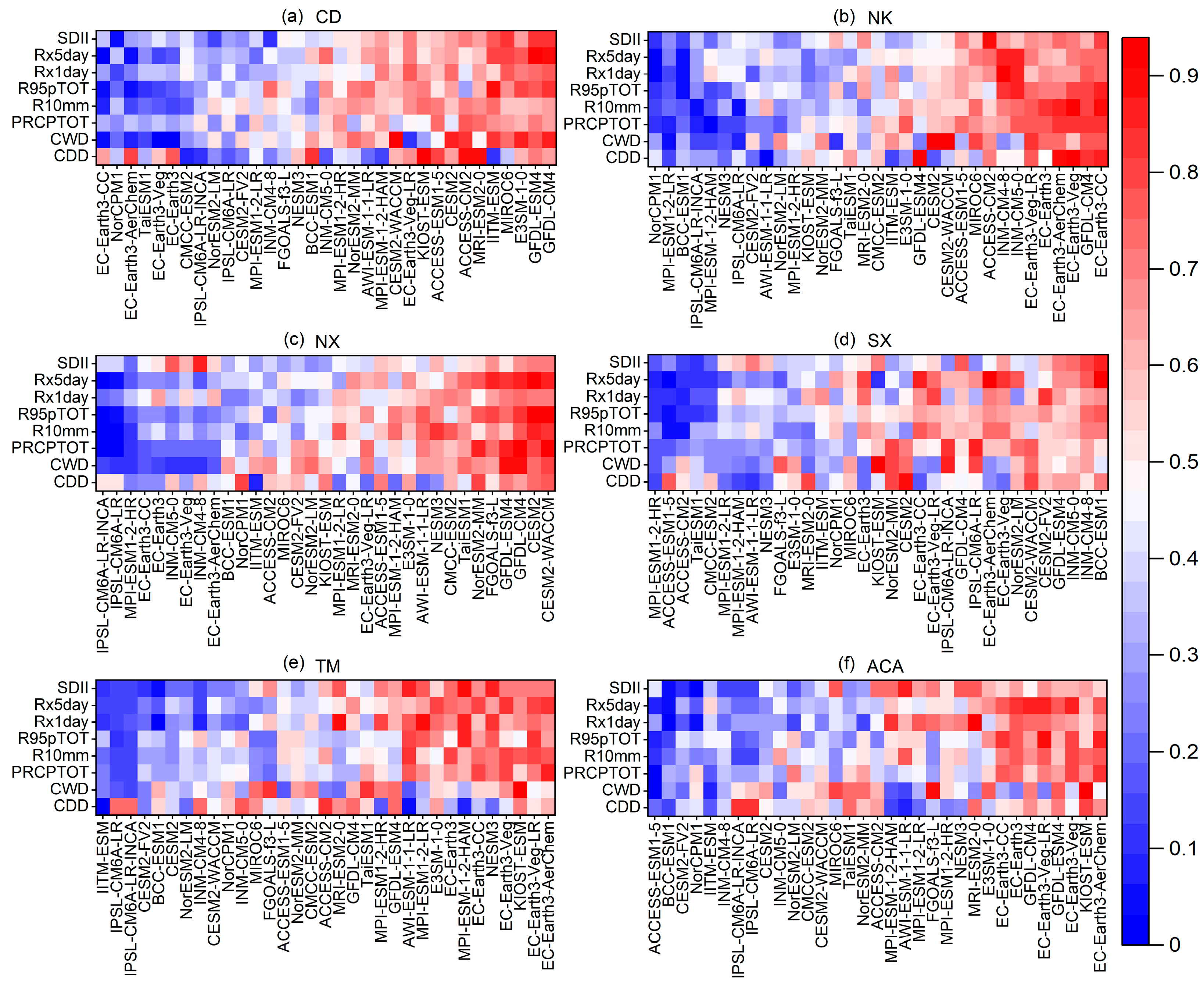
3.1. Spatial Evaluation

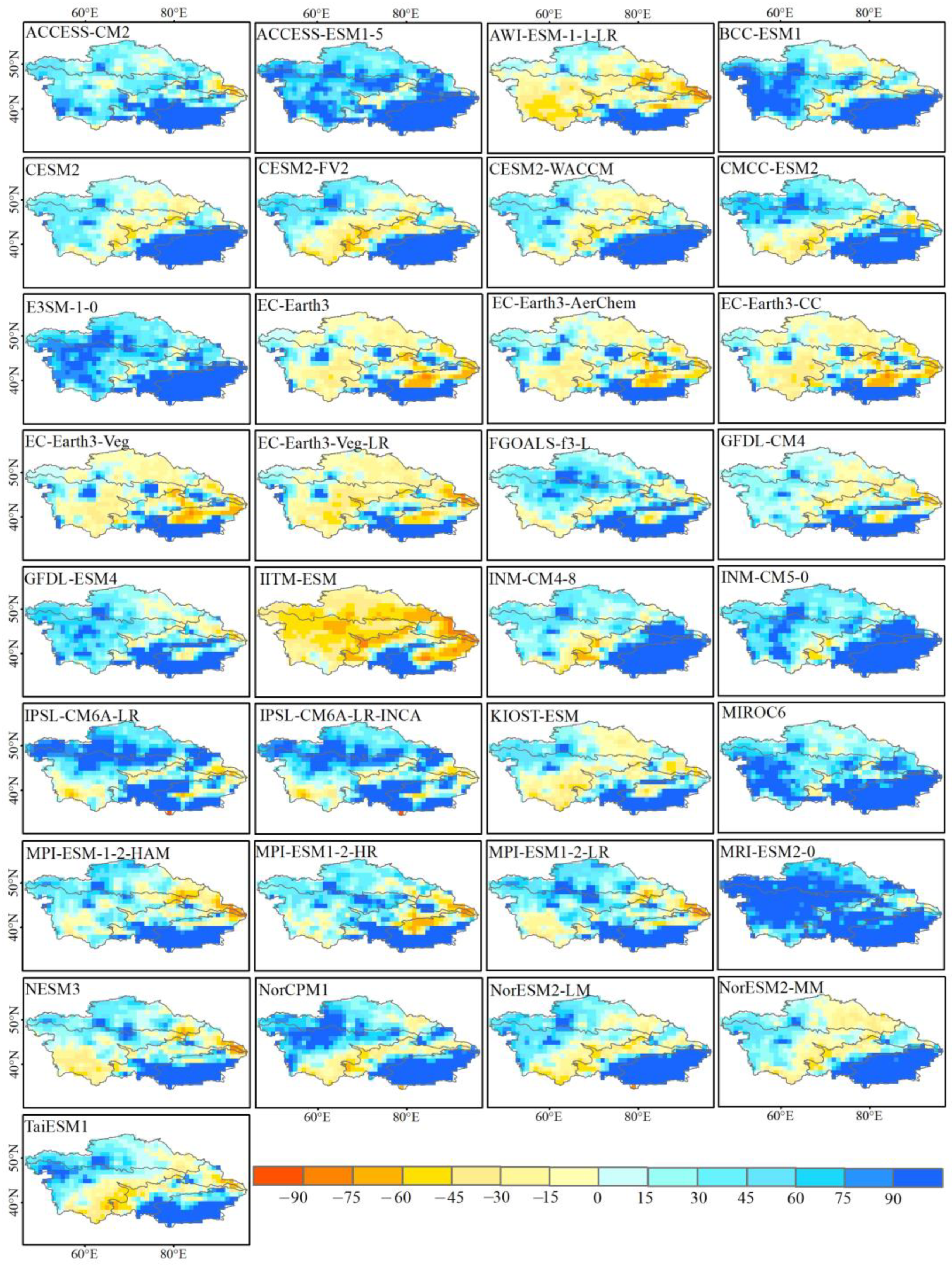
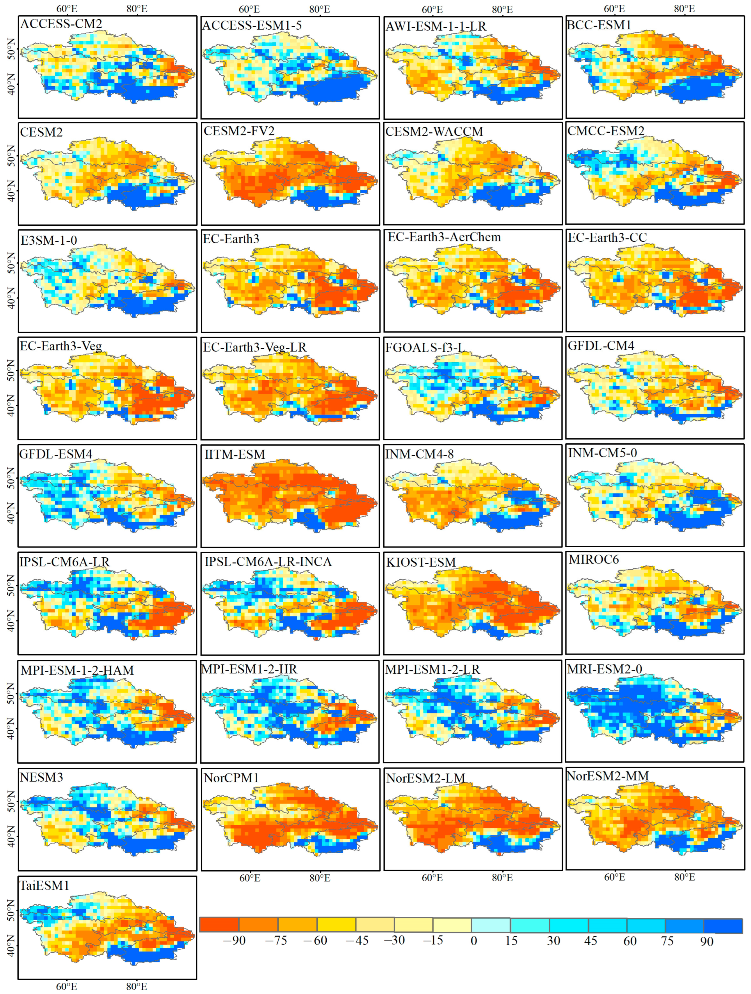
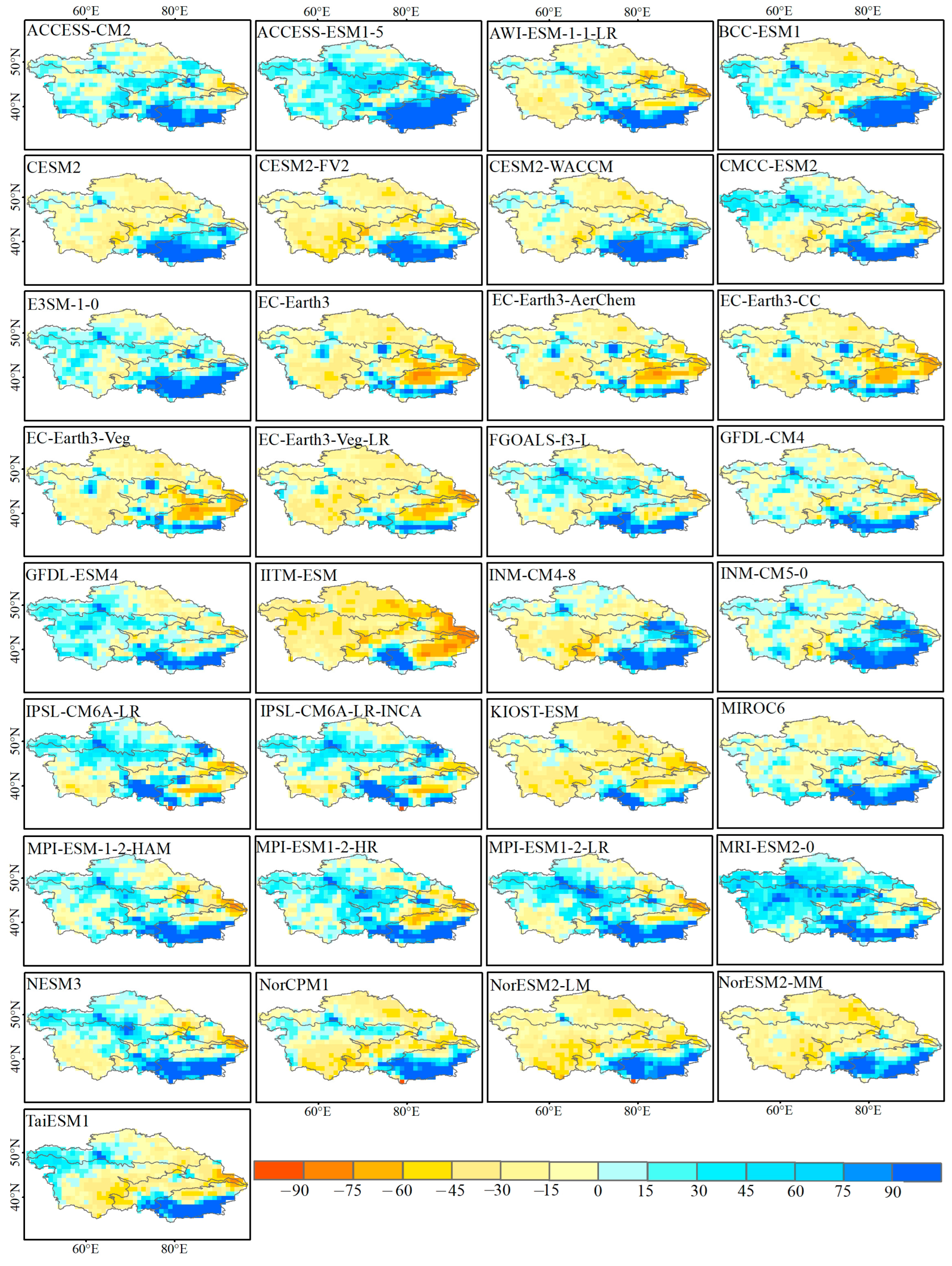
3.1.1. Spatial Bias Analysis

Figure 3, Figure 4, Figure 5 and Figure 6 show the percent bias of the spatial field over ACA extreme precipitation indices simulated by 33 GCMs during 1982–2014. The results show that most models can capture the spatial distribution of extreme precipitation better in NK and CD. In SX, almost all models simulate extreme precipitation indices with different degrees of wet bias, especially in the Kunlun Mountains region. Among the eight extreme indices, CMIP6 has the best ability to simulate SDII, with the percentage of spatial bias basically controlled at ±30% (Supplementary Material Figure S4). We also found that models from the same institution show similar regional biases and magnitudes in space.

For CDD (Figure 3), nearly half of the models could depict the spatial distribution of ACA, among which ACCESS-CM2, KIOST-ESM, MRI-ESM2-0 and TaiESM1 showed the best spatial performance, while AWI-ESM-1-1-LR, IITM-ESM, MPI-ESM-1-2-HAM, MPI-ESM1-2-HR, MPI-ESM1-2-LR and NESM3 showed great positive percentage biases in TM, Altai Mountains in NX and the western and the southwestern of CD. The models showed similar spatial biases for PRCPTOT (Figure 4), CWD and R95pTOT simulations, with high positive percentage biases in most areas (Supplementary Materials Figures S1 and S2). In contrast, most GCMs have high negative percentage biases for R10mm simulations, with dry bias, which substantially underestimates heavy rainfall in the region (Figure 5). Most models have a good simulation ability for Rx1day and are able to capture Rx1day, even in the complicated terrain of southern Xinjiang (Supplementary Material Figure S3). The higher positive bias for Rx5day is mainly in the Kunlun Mountains as well as in central Kazakhstan (Figure 6).

In general, these 33 GCMs have a certain ability to simulate the overall spatial distribution characteristics of extreme precipitation in ACA, with various performances in terms of precipitation intensity, precipitation duration and precipitation frequency. Unfortunately, no individual model was able to accurately capture all the spatial characteristics of the eight extreme precipitation indices in the ACA and each sub-region. Except for R10mm, EC-Earth3, EC-Earth3-CC, EC-Earth3-Veg-LR, KIOST-ESM and NorESM2-MM are the most powerful in simulating the other seven extreme precipitation indices.

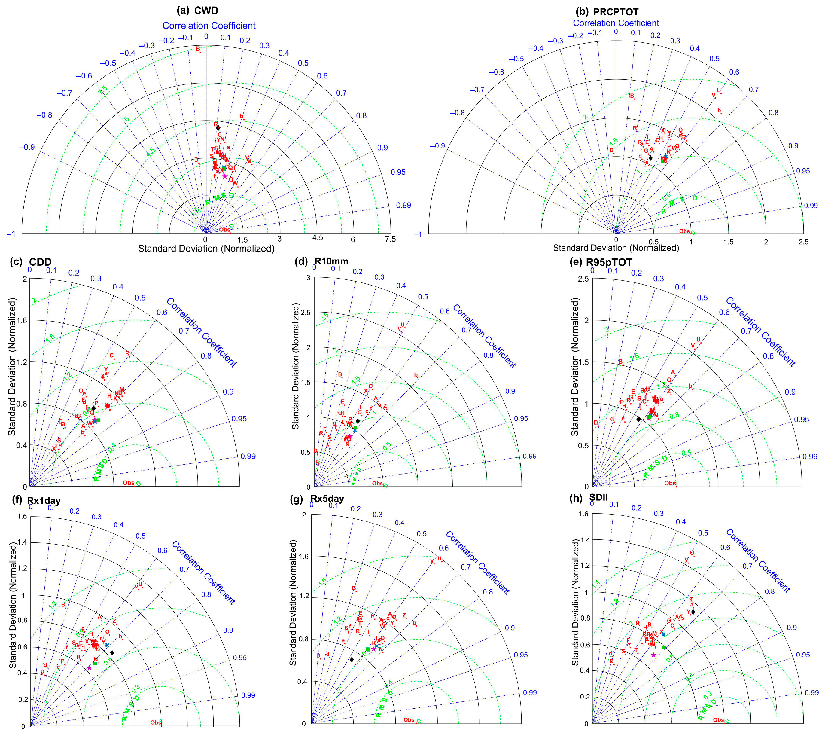
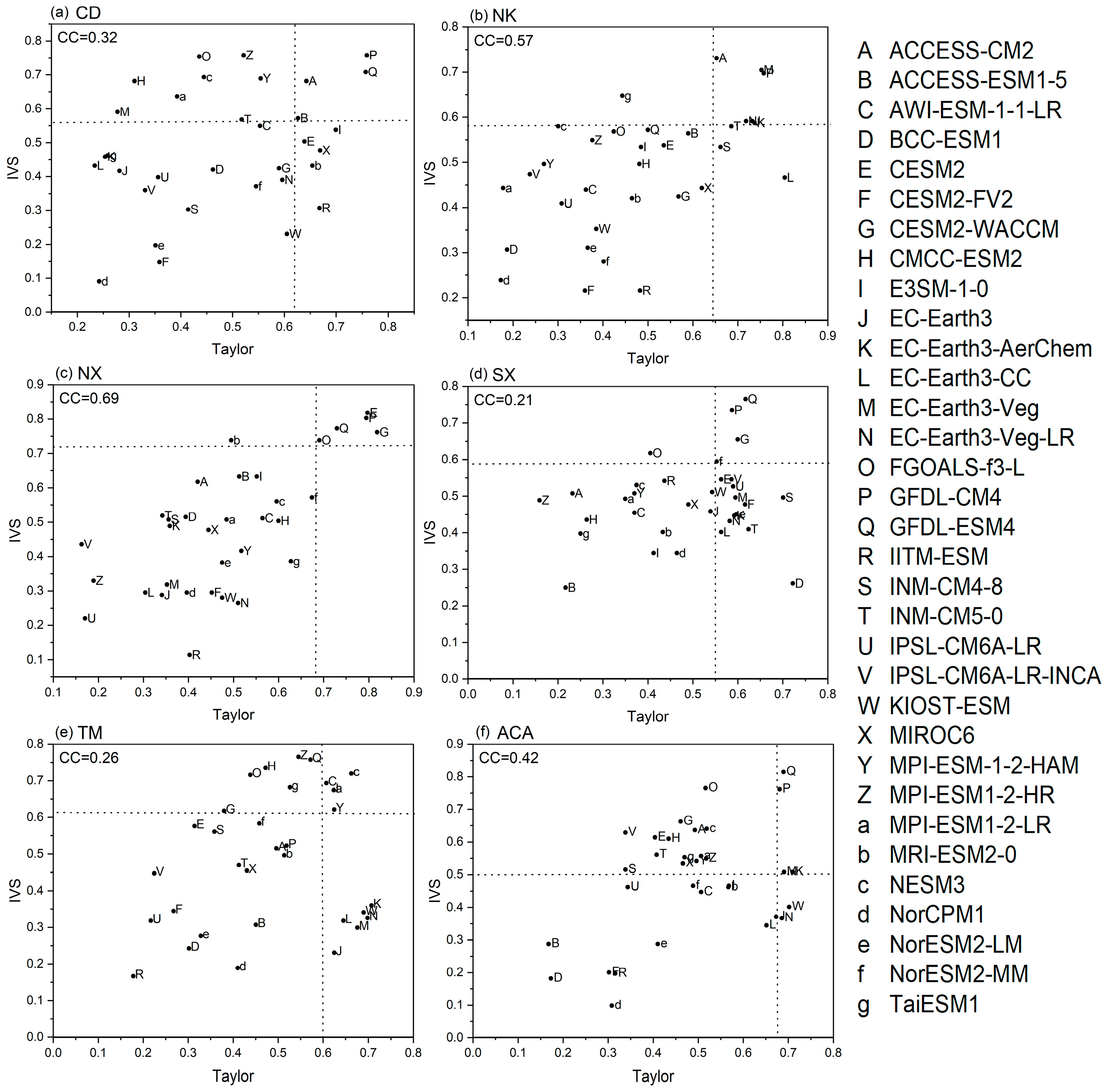
3.1.2. Taylor Diagram-Based Spatial Simulation Ability Analysis

To evaluate the ability of GCMs to simulate the spatial pattern of extreme precipitation indices, the Taylor diagram is further presented (Figure 7). It is found that CMIP6 models have the strongest ability to simulate the mean field of CDD and SDII; the CC of most models and the reference data are above 0.5, and the maximum RMSE is less than 1.3. For CWD, the consistency between model simulation and observation is poor on the whole, with the maximum CC being less than 0.6 (mostly between 0.1 and 0.4), and the σ and RMSE of most models are above 3. Except for ACCESS-ESM1-5, the remaining models have slight differences in terms of simulation ability, so they are relatively concentrated in the Taylor diagram. Both IPSL-CM6A-LR and IPSL-CM6A-LR-INCA show higher CC values with respect to the reference data in terms of extreme precipitation intensity (PRCPTOT, Rx1day, Rx5day), R95pTOT and extreme precipitation frequency (R10mm) in ACA, but they also have larger σ and RMSE values at the same time. The ability to simulate the R10mm spatial field varies, with the CC between models and the reference data ranging from 0.1 to 0.7, the RMSE being basically below 1.5 and σ ranging from 0.3 to 2.6. It is not hard to find that most GCMs have a similar spatial field simulation ability for Rx1day and Rx5day, with σ close to 1 and a smaller RMSE.

The MR₁ of 33 GCMs was calculated using three indices (CC, RMSE and σ) in the Taylor diagram. Figure 8 shows the ranking of the model’s ability to simulate the spatial field of eight extreme indices. The darker the red, the higher the value of MR₁ and the better the model performs. The results show that each model has a different ability to simulate the spatial fields of extreme precipitation indices in different regions. From the perspective of extreme precipitation indices, GCMs are more sensitive to the simulation of CDD and CWD in ACA and its sub-regions, with great uncertainty.

In terms of sub-regions, the model performs more stable extreme precipitation indices in NK. EC-Earth3-CC and GFDL-ESM4 have the best overall simulation ability performance, while NorCPM1 and MPI-ESM1-2-LR have the worst performance. In SX, TM and ACA, there are large differences in the spatial simulation abilities of the models for different extreme precipitation indices, such as BCC-ESM1 and EC-Earth3-Veg. Based on MR₁, the models with the best performance in simulating the spatial mean field of extreme precipitation indices at CD, NK, NX, SX, TM and ACA are GFDL-ESM4, EC-Earth3-CC, CESM2-WACCM, BCC-ESM1, EC-Earth3-AerChem and EC-Earth3-AerChem, respectively.

3.2. Temporal Evaluation

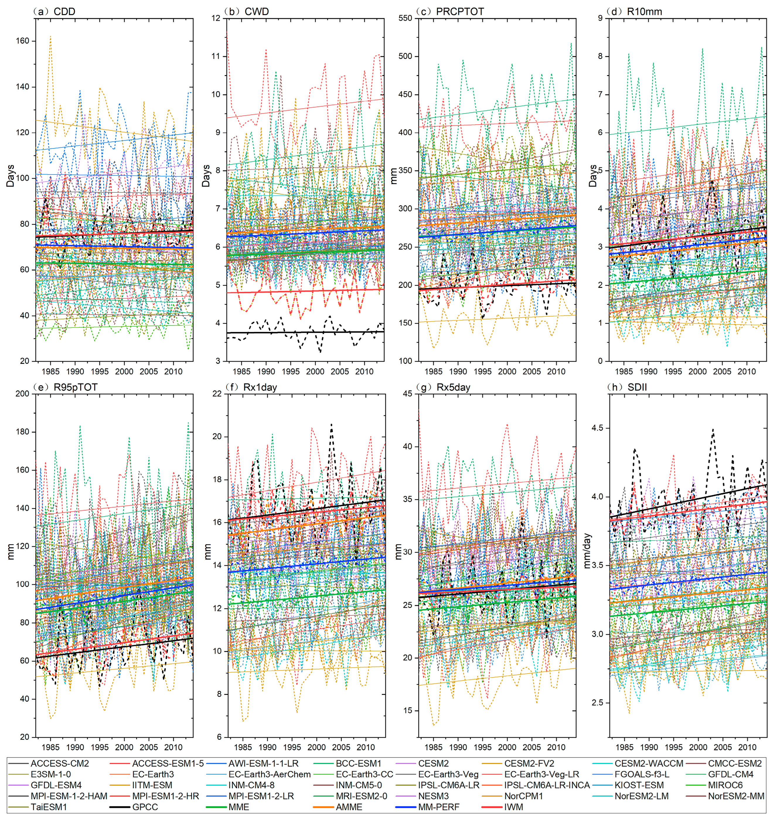
3.2.1. Trend Evaluation

The ability of the model to simulate the trend change in the extreme precipitation indices is an important aspect in testing the performance of the model. Figure 9 displays the annual variation trend of extreme precipitation indices simulated by 33 GCMs and the multi-model ensemble average.

Table 3. Regional average correlation coefficients between 33 GCMs’ simulations and GPCC observations. The highest and lowest CC values of each GCM over eight indices are marked by bold font and underline, respectively.

Model	CDD	CWD	PRCPTOT	R10mm	R95pTOT	Rx1day	Rx5day	SDII
ACCESS-CM2	0.245	0.476 **	0.350 *	0.146	0.264	−0.131	0.111	−0.181
ACCESS-ESM1-5	0.293	−0.004	−0.052	−0.212	−0.109	−0.208	−0.249	−0.016
AWI-ESM-1-1-LR	0.371 *	−0.084	−0.140	−0.065	−0.043	0.013	−0.190	−0.074
BCC-ESM1	−0.241	0.145	0.090	0.309	0.148	0.189	0.368 *	0.198
CESM2	0.064	−0.117	0.168	0.168	0.221	−0.014	0.091	0.122
CESM2-FV2	0.427 *	−0.128	0.192	0.169	0.151	0.033	−0.004	0.087
CESM2-WACCM	−0.068	−0.109	0.045	0.122	0.188	0.165	0.181	0.257
CMCC-ESM2	0.046	−0.022	0.007	−0.029	0.028	0.097	0.130	0.041
E3SM-1-0	0.306	−0.232	0.052	−0.099	−0.069	−0.217	−0.335	−0.059
EC-Earth3	0.010	0.018	0.053	0.108	0.140	0.027	−0.022	0.164
EC-Earth3-AerChem	−0.479 **	0.017	−0.168	−0.019	−0.043	−0.139	−0.051	0.009
EC-Earth3-CC	0.247	0.146	0.290	0.223	0.243	0.159	0.159	0.112
EC-Earth3-Veg	−0.237	−0.155	0.002	0.105	0.122	0.247	0.097	0.368 *
EC-Earth3-Veg-LR	0.122	−0.020	0.193	0.108	0.110	0.089	−0.047	0.041
FGOALS-f3-L	−0.134	−0.015	0.100	0.170	0.189	0.123	0.160	0.277
GFDL-CM4	0.049	−0.051	−0.273	−0.229	−0.159	−0.155	−0.154	0.069
GFDL-ESM4	0.097	−0.303	−0.093	0.060	0.031	0.081	0.094	0.161
IITM-ESM	0.088	−0.062	0.217	0.187	0.260	0.130	0.138	0.305
INM-CM4-8	−0.044	0.272	0.234	0.170	0.252	0.079	0.080	0.121
INM-CM5-0	−0.013	0.235	0.163	0.231	0.273	0.159	0.232	0.314
IPSL-CM6A-LR	−0.012	−0.173	0.187	0.194	0.178	−0.079	−0.049	0.080
IPSL-CM6A-LR-INCA	0.164	0.164	−0.219	−0.303	−0.164	0.026	0.193	0.075
KIOST-ESM	−0.038	0.129	−0.227	−0.059	−0.257	−0.252	−0.034	−0.227
MIROC6	0.021	−0.043	0.123	0.193	0.186	0.176	0.100	0.209
MPI-ESM-1-2-HAM	−0.121	−0.207	−0.191	−0.088	−0.021	−0.105	−0.176	0.067
MPI-ESM1-2-HR	−0.141	−0.286	−0.017	0.102	0.148	0.234	0.050	0.185
MPI-ESM1-2-LR	−0.211	−0.095	−0.029	0.122	0.141	0.109	0.086	0.342
MRI-ESM2-0	0.102	0.086	0.094	0.072	0.144	0.301	0.288	0.186
NESM3	−0.101	−0.035	0.225	0.150	0.110	0.037	0.087	−0.016
NorCPM1	0.081	0.289	0.044	0.119	0.143	0.067	0.221	0.217
NorESM2-LM	−0.359 *	−0.188	−0.231	−0.172	−0.198	0.008	−0.162	−0.012
NorESM2-MM	0.025	0.023	0.118	0.191	0.179	0.177	0.147	0.146
TaiESM1	0.145	0.011	0.108	0.159	0.127	0.127	0.076	0.309

Note: * means it passes the 95% significance test, ** means it passes the 99% significance test.

shows the correlation coefficients of the regional average between 33 CMIP6 models and GPCC.

Compared with the reference data, most CMIP6 models are able to detect the increasing trends of CWD, PRCPTOT, R10mm, R95pTOT, Rx1day, Rx5day and SDII, but for CDD, more than half of the simulated values of GCMs are contrary to the trends observed by GPCC. In terms of the magnitude of trend deviation, the vast majority of models underestimate the growth trends of CDD (0.9 days/10a), R10mm (0.2 days/10a), Rx1day (0.3 mm/10a) and SDII (0.07 mm/day/10a). About one-third of the models overestimate the trends of CWD (0.008 days/10a), PRCPTOT (2.5 mm/10a), R95pTOT (3.2 mm/10a) and Rx5day (0.4 days/10a). Compared with the spatial pattern, models have a relatively poor ability to simulate the trends of extreme precipitation indices.

Taking CDD as an example, CESM2-FV2, E3SM-1-0 and AWI-ESM-1-1-LR all have high correlation coefficients with the reference data (0.43, 0.31 and 0.37, respectively), but AWI-ESM-1-1-LR largely overestimates the variation trend of CDD, and CESM2-FV2 underestimates the trend of CDD. In contrast, E3SM-1-0 has a higher correlation coefficient and is closest to the variation trend of GPCC. Therefore, we believe that E3SM-1-0 has the best ability to simulate the trend change of CDD. For the remaining seven extreme precipitation indices, the models with the best simulation abilities are ACCESS-CM2, INM-CM4-8, EC-Earth3-CC, INM-CM4-8, MPI-ESM1-2-HR, MRI-ESM2-0 and IITM-ESM.

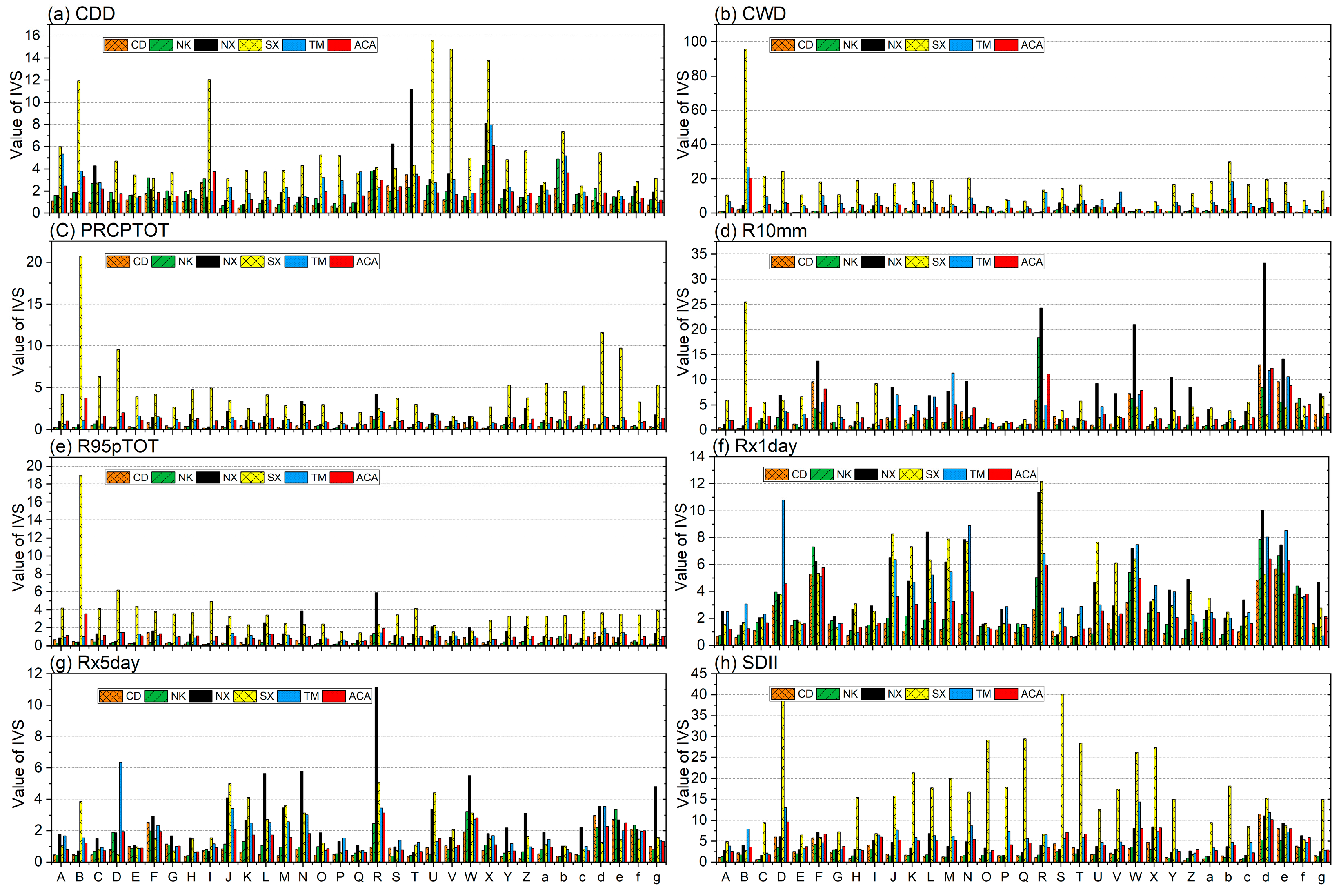
3.2.2. Evaluation of Interannual Variability

According to Equation (2) in Section 2.3.2, we calculate the interannual variability skill score of the model spatial field relative to the GPCC observation field (Figure 10). Similar to the simulation results in the Taylor diagram, the CMIP6 model has the worst simulation of CWD in ACA (IVS between 0 and 20.4), followed by R10mm (IVS between 0 and 12.3). On the contrary, PRCPTOT, R95pTOT and Rx5day have better simulations of interannual variability. Furthermore, it is difficult to capture the interannual variability of the SDII observation field in ACA, and the difference between the models is not significant.

From the point of view of each sub-region, the interannual variability skill scores of models are relatively small in NK and CD, with the IVS of extreme precipitation indices ranging from 0 to 13 and from 0 to 8.5, respectively, except for IITM-ESM. GCMs have the worst ability to simulate the interannual variability of extreme precipitation indices in SX, especially in CWD and SDII. The IVS values of CWD simulated by the model are relatively low in NX but have limited ability to capture interannual variability for R10mm and Rx1day, with significant differences in the simulation ability among models. GCMs perform better overall in reproducing interannual variability for PRCPTOT and R95pTOT in TM, with IVS values not exceeding 2.5.

In general, CMIP6 models are basically able to reproduce the interannual variability of PRCPTOT, R95pTOT and Rx5day in ACA and sub-regions, but the interannual variability of R10mm, SDII and CWD need to be improved. The best-performing models in capturing the interannual variability of extreme precipitation indices in CD, NK, NX, SX, TM and ACA are: MPI-ESM1-2-HR, ACCESS-CM2, GFDL-CM4, NorESM2-MM, MPI-ESM1-2-HR and FGOALS-f3-L, respectively.

3.3. Overall Model Performance

Given the inconsistency of spatial and temporal model rankings, in order to more intuitively determine the spatio-temporal simulation ability of the models, this study calculated MR based on Taylor and IVS for a comprehensive evaluation of the models (Figure 11). The study calculated MR based on Taylor and IVS to more intuitively determine the spatio-temporal simulation ability of the models. Taylor diagram-based MR₁ and IVS based MR₂ are significantly correlated in NK, NX and ACA; the correlation coefficients are 0.57, 0.69 and 0.42, respectively (all passed the 95% significance test), while the spatial pattern and interannual variability of extreme precipitation indices simulated by the models in CD, SX and TM were not consistent, with correlation coefficients of 0.32, 0.21 and 0.26, respectively. The points on the plane were divided into four quadrants. Models in the upper right quadrant have better spatial and temporal simulation ability, while models in the lower left quadrant have the worst simulation ability. The MR₁ and MR₂ correlations of NK and TM are not high, but the best-performing models are more concentrated.

Considering the simulation capability in terms of spatial and temporal variability, ACCESS-CM2, ACCESS-ESM1-5, GFDL-CM4 and GFDL-ESM4 perform best in CD, among which ACCESS-CM2 and GFDL-CM4 also perform better in NK and are more suitable for extreme precipitation simulation in flat areas. In addition, models of the EC-Earth-Consortium institution (e.g., EC-Earth3-Veg, etc.) all perform better in NK. GFDL-CM4, GFDL-ESM4 and CESM2-WACCM are more suitable for Xinjiang (SX and NX). For mountainous regions (TM), the models simulated extreme precipitation indices that are less consistent than those in other regions in terms of the spatial pattern and interannual variability, and the best-simulated models are NESM3, AWI-ESM-1-1-LR, MPI-ESM1-2-LR, MPI-ESM-1-2-HAM and E3SM-1-0. Across the ACA, the best-performing models are GFDL-CM4, GFDL-ESM4, EC-Earth3-Veg and EC-Earth3-AerChem.

3.4. Multi-Modal Ensemble Performance Evaluation

Compared with individual models, multi-model ensemble methods have significantly better simulation ability for extreme precipitation spatial fields in ACA. Except for CWD, the CCs of the four multi-model ensemble simulations with reference data are basically above 0.6, and the RMSE is significantly reduced, while σ is closer to 1 (Figure 7). Figure 12 shows the spatial percentage biases of eight extreme precipitation indices simulated by four multi-model ensemble methods versus those observed by GPCC.

Due to the inherent limitations of GCMs, even with different multi-model ensemble methods, the improvement of CWD, PRCPTOT, R10mm and R95pTOT is still very limited, and there are still very large wet biases in the southeastern TM and the southern and central SX. Two unweighted schemes have a similar simulation performance on CDD, CWD, PRCPTOT and R95pTOT. AMME is better than MME for R10mm, but MME is better than AMME in simulating extreme precipitation intensity SDII. Among the weighted multi-model ensemble methods, the spatial bias of the extreme precipitation indices simulated by MM-PERF is slightly smaller than that of unweighted AMME in ACA. With the exception of CDD, which has large biases in TM and NX, IWM-simulated extreme precipitation indices have an overall smaller spatial percentage bias than the other three multi-model ensembles.

In conclusion, four multi-model ensemble methods have a certain ability to simulate extreme precipitation over ACA, and the performance of weighted multi-model ensemble is better than that of equal-weight multi-model ensemble. IWM has a relatively better spatial simulation ability for extreme precipitation indices.

Multi-model ensemble can effectively reduce the systematic bias and variability within individual models. By comparing four multi-model ensemble methods, simulations of different extreme precipitation indices are improved to varying degrees (Figure 13). Compared to individual model simulations (Supplementary Material Figure S5), the bias of extreme precipitation indices across ACA was reduced by at least 50%, which is evident in both PRCPTOT and R95pTOT simulations.

From the perspective of correlation, the weighted multi-model ensemble simulation effect has improved significantly, and the correlation coefficient can reach up to 0.7. In terms of the multimodal ensemble method performance, weighted multi-model ensemble effects are better than equal-weighted ensemble effects, and the temporal variation trend of IWM is closest to the reference data (Figure 8). The uncertainty of simulated precipitation duration (CDD, CWD), PRCPTOT and R95PTOT in MME was slightly less than that in AMME but less than that in R10mm, Rx1day, Rx1day and SDII. Although the MM-PERF method can also reduce the uncertainty of extreme precipitation simulation, the improvement effect is not as good as that of IWM. The results of the partitioning show that there are still great uncertainties in the simulation of extreme precipitation in SX and TM.

4. Discussion

By comparing the spatio-temporal simulation performance between CMIP6 models, it is found that most models have a large wet bias for TM and SX, which is consistent with the findings of Dong et al. [9,50], while the simulation ability is better in plain regions. Liu et al. found that it was difficult for the CMIP6 model to simulate the overall spatial pattern of extreme precipitation in early spring and late winter, the inter-model variability of regional bias in summer was large and the areas of inconsistency that emerge always contain most of Xinjiang or its surrounding mountain regions [57].This may be due to the complex conditions in the Tianshan Mountains and Southern Xinjiang, and the coarse resolutions of CMIP6 models make it difficult to capture the precipitation variability in this region. For extreme precipitation indices, most models overestimate the mean and variability of total precipitation PRCPTOT and CWD but underestimate the mean and variability of CDD and SDII, and a similar situation was found in East Africa and contiguous regions of the United States [58,59]. Luo and Guo [60] pointed out that improved resolution has obvious advantages in simulating extreme precipitation, especially in some areas with complex topography. However, this explanation does not seem to hold up in some tropical regions, such as East Africa [58]. In this study, some models with a lower resolution are better than those with a higher resolution (such as IITM-ESM) in capturing the spatial distribution of extreme precipitation. As a result, the resolution of the model cannot fully explain the performance of the model, but the setting of the parameterization scheme of the model itself, the physical process and other factors should also be taken into account [61,62].

Extreme precipitation is generally related to the convection and cloud microphysics [63]. It is difficult to attribute the difference in the simulation ability of each model in different regions. To reduce the uncertainty of future climate projection, scholars have been working on an ideal model ensemble method, but there is still a dispute over the weight of climate models in the world [56,64]. Moreover, a weighted multi-model ensemble approach is very sensitive to the indicators used, and the selection of indexes can directly lead to the quality of simulation results. In this paper, four statistical indicators (CC, RMSE, RB and σ) are mainly used in the MM-PERF in the weighted multi-model ensemble method, and the IWM scheme outperforms the MM-PERF overall. However, if other indicators or methods are used, the results may be different. For example, Zhang et al. used a weighted multi-model ensemble to project the changes in extreme precipitation in Central Asia under different temperature rises and found that there was a robust consistency between the changes in precipitation intensity and the cumulative one, but the noise generated by the uncertainty between the models covered the signals of CDD changes [39]. In addition, the spread of summer precipitation extremes over northern Central Asia is large [40]. The simulation ability of models should be understood in the context of specific variables and spatio-temporality [65,66].

Currently, the improvement of the model simulation ability is mainly focused on reducing uncertainty in climate change prediction by establishing some relationship between observations and simulations [67,68]. However, this method is vulnerable to the influence of the quality of observed data, physical processes and even the subjective consciousness of researchers [64]. In addition, a simple assessment of the model’s performance in the current climate is not sufficient to judge the model’s performance [69]. Hence, the in-depth understanding and elimination of the CMIP6 models’ bias is the key to improving the accuracy of regional climate projection, and it is also the focus of future research efforts. Zhang et al. used downscaling and two methods of local intensity scaling (LOCI) and quantile mapping (QM) and greatly reduced the deviation in extreme precipitation simulation [70]. Other multi-model ensemble methods or bias correction of the data, such as machine learning and downscaling, could be tried in the future to reduce model uncertainty in simulations and projections.

5. Conclusions

In this paper, based on the GPPC V2020 daily precipitation data products and 33 GCMs datasets, eight extreme precipitation indices defined by ETCCDI were selected to quantitatively and comprehensively evaluate the spatial and temporal simulation ability of the models for extreme precipitation in ACA and each sub-region. By comparing and analyzing the simulation performance of four multi-model ensemble averaging methods and individual models, the models and multi-model ensemble averaging methods with relatively reliable simulation effects are selected. The main conclusions are as follows:

(1) In terms of spatial simulation, most models can simulate the spatial characteristics of extreme precipitation indices well. However, the simulation ability of the models varies for different indices. The models have a stronger simulation ability for CDD and SDII, and the correlation coefficients between the climate mean fields of extreme precipitation indices simulated by most of the models and the extreme precipitation indices observed by the reference data exceed 0.6. Relatively speaking, the models have poor simulation ability for CWD and R10mm, the consistency of spatial distribution characteristics with the reference data is weak and the simulation ability varies greatly between models.

(2) As for temporal variability simulation ability, the linear variation trends of the extreme precipitation indices simulated by the models are mostly consistent with the reference data in ACA, but the simulation ability is weak in terms of trend intensity. As for the interannual variability skill scores of each sub-region, the low IVS scores (0–8.5 and 0–13, respectively) of the models in CD and NK indicated a relatively good simulation. However, it performs the worst in terms of reproducing the interannual variability of extreme precipitation in the SX. GCMs have limited ability to capture the interannual variability of R10mm, SDII and CWD in the ACA and each sub-region.

(3) Considering the ability of the models to simulate the spatial pattern and interannual variability of the extreme precipitation indices, ACCESS-CM2 and GFDL-CM4 performed better in the relatively flat CD and NK. NESM3, AWI-ESM-1-1-LR, MPI-ESM1-2-LR, MPI-ESM-1-2-HAM and E3SM-1-0 have relatively good simulation capability in the TM region. For the whole ACA, the best-performing models are GFDL-CM4, GFDL-ESM4, EC-Earth3-Veg and EC-Earth3-AerChem.

(4) Comparing the effects of four different multi-model ensemble averaging methods, it is found that the multi-model ensemble averaging methods have a significant improvement in the spatial and temporal simulation ability of extreme precipitation indices and can effectively reduce the internal bias and variability of individual models (especially in CD and NK). However, there are still large uncertainties in the extreme precipitation simulation in SX and TM. The non-equally weighted model ensemble averaging method is superior to the unweighted multi-model ensemble methods, among which IWM has the most obvious enhancement of the simulation ability of extreme precipitation indices and the best performance.

References

1. World Meteorological Organization (WMO). State of the Global Climate 2021; World Meteorological Organization (WMO): Geneva, Switzerland, 2022; p. 2. [Google Scholar]
2. Donat, M.G.; Lowry, A.L.; Alexander, L.V.; O’Gorman, P.A.; Maher, N. More extreme precipitation in the world’s dry and wet regions. Nat. Clim. Chang. 2016, 6, 508–513. [Google Scholar] [CrossRef]
3. Gessner, U.; Naeimi, V.; Klein, I.; Kuenzer, C.; Klein, D.; Dech, S. The relationship between precipitation anomalies and satellite-derived vegetation activity in Central Asia. Glob. Planet. Chang. 2013, 110, 74–87. [Google Scholar] [CrossRef]
4. Maxwell, S.L.; Butt, N.; Maron, M.; McAlpine, C.A.; Chapman, S.; Ullmann, A.; Segan, D.B.; Watson, J.E.M. Conservation implications of ecological responses to extreme weather and climate events. Divers. Distrib. 2018, 25, 613–625. [Google Scholar] [CrossRef]
5. Runde, I.; Zobel, Z.; Schwalm, C. Human and natural resource exposure to extreme drought at 1.0 °C–4.0 °C warming levels. Environ. Res. Lett. 2022, 17, 064005. [Google Scholar] [CrossRef]
6. Garreaud, R.D.; Boisier, J.P.; Rondanelli, R.; Montecinos, A.; Sepúlveda, H.H.; Veloso-Aguila, D. The Central Chile Mega Drought (2010–2018): A climate dynamics perspective. Int. J. Climatol. 2019, 40, 421–439. [Google Scholar] [CrossRef]
7. Zhao, Z.; Luo, Y.; Huang, J. The detection of the CMIP5 climate model to see the development of CMIP6 earth system models. Clim. Chang. Res. 2018, 14, 643–648. [Google Scholar] [CrossRef]
8. Chen, H.; Sun, J.; Lin, W.; Xu, H. Comparison of CMIP6 and CMIP5 models in simulating climate extremes. Sci. Bull. 2020, 65, 1415–1418. [Google Scholar] [CrossRef]
9. Dong, T.; Dong, W. Evaluation of extreme precipitation over Asia in CMIP6 models. Clim. Dyn. 2021, 57, 1751–1769. [Google Scholar] [CrossRef]
10. Kim, Y.-H.; Min, S.-K.; Zhang, X.; Sillmann, J.; Sandstad, M. Evaluation of the CMIP6 multi-model ensemble for climate extreme indices. Weather Clim. Extrem. 2020, 29, 100269. [Google Scholar] [CrossRef]
11. Rivera, J.A.; Arnould, G. Evaluation of the ability of CMIP6 models to simulate precipitation over Southwestern South America: Climatic features and long-term trends (1901–2014). Atmos. Res. 2020, 241, 104953. [Google Scholar] [CrossRef]
12. Fan, X.; Miao, C.; Duan, Q.; Shen, C.; Wu, Y. The performance of CMIP6 versus CMIP5 in simulating temperature extremes over the global land surface. J. Geophys. Res. Atmos. 2020, 125, e2020JD033031. [Google Scholar] [CrossRef]
13. Gupta, V.; Singh, V.; Jain, M.K. Assessment of precipitation extremes in India during the 21st century under SSP1-1.9 mitigation scenarios of CMIP6 GCMs. J. Hydrol. 2020, 590, 125422. [Google Scholar] [CrossRef]
14. Li, J.; Huo, R.; Chen, H.; Zhao, Y.; Zhao, T. Comparative Assessment and Future Prediction Using CMIP6 and CMIP5 for Annual Precipitation and Extreme Precipitation Simulation. Front. Earth Sci. 2021, 9, 687976. [Google Scholar] [CrossRef]
15. Guan, J.; Yao, J.; Li, M.; Li, D.; Zheng, J. Historical changes and projected trends of extreme climate events in Xinjiang, China. Clim. Dyn. 2022, 58, 1753–1774. [Google Scholar] [CrossRef]
16. Erlandsen, H.B.; Parding, K.M.; Benestad, R.; Mezghani, A.; Pontoppidan, M. A Hybrid Downscaling Approach for Future Temperature and Precipitation Change. J. Appl. Meteorol. Climatol. 2020, 59, 1793–1807. [Google Scholar] [CrossRef]
17. Rashid, M.B.; Hossain, S.S.; Mannan, M.A.; Parding, K.M.; Hygen, H.O.; Benestad, R.E.; Mezghani, A. Climate change projections of maximum temperature in the pre-monsoon season in Bangladesh using statistical downscaling of global climate models. Adv. Sci. Res. 2021, 18, 99–114. [Google Scholar] [CrossRef]
18. Jiang, S.; Jiang, Z.; Li, W. Evaluation of the Extreme Temperature and Its Trend in China Simulated CMIP5 models. Clim. Chang. Res. 2017, 13, 11–24. [Google Scholar] [CrossRef]
19. Ge, F.; Zhu, S.; Luo, H.; Zhi, X.; Wang, H. Future changes in precipitation extremes over Southeast Asia: Insights from CMIP6 multi-model ensemble. Environ. Res. Lett. 2021, 16, 024013. [Google Scholar] [CrossRef]
20. Jiang, W.H.; Chen, H.P. Assessment and projection of changes in temperature extremes over the mid-high latitudes of Asia based on CMIP6 models. Trans. Atmos. Sci. 2021, 44, 592–603. [Google Scholar] [CrossRef]
21. Liu, Z.; Lu, J.; Huang, J.; Chen, X.; Zeng, Q. Potential evapotranspiration and drought effects of Poyang Lake Basin based on global climate model aggregation. Acta Ecol. Sin. 2021, 41, 6936–6948. [Google Scholar]
22. Bishop, C.H.; Abramowitz, G. Climate model dependence and the replicate Earth paradigm. Clim. Dyn. 2012, 41, 885–900. [Google Scholar] [CrossRef]
23. Bai, H.; Xiao, D.; Wang, B.; Liu, D.L.; Feng, P.; Tang, J. Multi-model ensemble of CMIP6 projections for future extreme climate stress on wheat in the North China plain. Int. J. Climatol. 2020, 41, E171–E186. [Google Scholar] [CrossRef]
24. Zarrin, A.; Dadashi-Roudbari, A.; Hassani, S. Historical variability and future changes in seasonal extreme temperature over Iran. Theor. Appl. Climatol. 2021, 146, 1227–1248. [Google Scholar] [CrossRef]
25. Ma, Q.; Zhang, J.; Game, A.T.; Chang, Y.; Li, S. Spatiotemporal variability of summer precipitation and precipitation extremes and associated large-scale mechanisms in Central Asia during 1979–2018. J. Hydrol. X 2020, 8, 100061. [Google Scholar] [CrossRef]
26. Yao, J.; Zeng, Y.; Li, J.; Yang, L. A Review of Dry-Wet Climate Change and Extreme Precipitation in Central Asia. Adv. Meteorol. Sci. Technol. 2020, 10, 7–14. [Google Scholar] [CrossRef]
27. Liang-Liang, L.; Jian, L.; Ru-Cong, Y. Evaluation of CMIP6 HighResMIP models in simulating precipitation over Central Asia. Adv. Clim. Chang. Res. 2022, 13, 1–13. [Google Scholar] [CrossRef]
28. Zhang, M.; Chen, Y.; Shen, Y.; Li, B. Tracking climate change in Central Asia through temperature and precipitation extremes. J. Geogr. Sci. 2019, 29, 3–28. [Google Scholar] [CrossRef]
29. Hu, W.; Yao, J.; He, Q.; Chen, J. Changes in precipitation amounts and extremes across Xinjiang (northwest China) and their connection to climate indices. PeerJ 2021, 9, e10792. [Google Scholar] [CrossRef]
30. Tian, Y.; Yan, Z.; Li, Z. Spatial and Temporal Variations of Extreme Precipitation in Central Asia during 1982–2020. Atmosphere 2021, 13, 60. [Google Scholar] [CrossRef]
31. Zhang, X.; Chen, Y.; Fang, G.; Li, Y.; Li, Z.; Wang, F.; Xia, Z. Observed changes in extreme precipitation over the Tienshan Mountains and associated large-scale climate teleconnections. J. Hydrol. 2022, 606, 127457. [Google Scholar] [CrossRef]
32. Zhang, M.; Chen, Y.; Shen, Y.; Li, Y. Changes of precipitation extremes in arid Central Asia. Quat. Int. 2017, 436, 16–27. [Google Scholar] [CrossRef]
33. Xu, P.; Wang, L.; Ming, J. Central Asian Precipitation Extremes Affected by an Intraseasonal Planetary Wave Pattern. J. Clim. 2022, 35, 2603–2616. [Google Scholar] [CrossRef]
34. Khadgarai, S.; Kumar, V.; Pradhan, P.K. The Connection between Extreme Precipitation Variability over Monsoon Asia and Large-Scale Circulation Patterns. Atmosphere 2021, 12, 1492. [Google Scholar] [CrossRef]
35. Jiang, J.; Zhou, T.; Chen, X.; Zhang, L. Future changes in precipitation over Central Asia based on CMIP6 projections. Environ. Res. Lett. 2020, 15, 054009. [Google Scholar] [CrossRef]
36. Zhao, Y.; Qian, C.; Zhang, W.; He, D.; Qi, Y. Extreme temperature indices in Eurasia in a CMIP6 multi-model ensemble: Evaluation and projection. Int. J. Climatol. 2021, 41, 5368–5385. [Google Scholar] [CrossRef]
37. Fan, X.; Duan, Q.; Shen, C.; Wu, Y.; Xing, C. Evaluation of historical CMIP6 model simulations and future projections of temperature over the Pan-Third Pole region. Environ. Sci. Pollut. Res. Int. 2022, 29, 26214–26229. [Google Scholar] [CrossRef]
38. Lin, W.; Chen, H. Assessment of model performance of precipitation extremes over the mid-high latitude areas of Northern Hemisphere: From CMIP5 to CMIP6. Atmos. Ocean. Sci. Lett. 2020, 13, 598–603. [Google Scholar] [CrossRef]
39. Zhang, J.; Wang, F. Future changes in extreme precipitation in central Asia with 1.5–4 °C global warming based on Coupled Model Intercomparison Project Phase 6 simulations. Int. J. Climatol. 2022, 42, 8509–8525. [Google Scholar] [CrossRef]
40. Dike, V.N.; Lin, Z.; Fei, K.; Langendijk, G.S.; Nath, D. Evaluation and multimodel projection of seasonal precipitation extremes over central Asia based on CMIP6 simulations. Int. J. Climatol. 2022, 42, 7228–7251. [Google Scholar] [CrossRef]
41. Hu, Z.; Zhou, Q.; Chen, X.; Li, J.; Li, Q.; Chen, D.; Liu, W.; Yin, G. Evaluation of three global gridded precipitation data sets in central Asia based on rain gauge observations. Int. J. Climatol. 2018, 38, 3475–3493. [Google Scholar] [CrossRef]
42. Yu, Y.; Schneider, U.; Yang, S.; Becker, A.; Ren, Z. Evaluating the GPCC Full Data Daily Analysis Version 2018 through ETCCDI indices and comparison with station observations over mainland of China. Theor. Appl. Climatol. 2020, 142, 835–845. [Google Scholar] [CrossRef]
43. Dilinuer, T.; Yao, J.; Chen, J.; Zhao, Y.; Mao, W.; Li, J.; Yang, L. Systematical Evaluation of Three Gridded Daily Precipitation Products Against Rain Gauge Observations Over Central Asia. Front. Earth Sci. 2021, 9, 699628. [Google Scholar] [CrossRef]
44. Song, L.; Xu, C.; Long, Y.; Lei, X.; Suo, N.; Cao, L. Performance of Seven Gridded Precipitation Products over Arid Central Asia and Subregions. Remote Sens. 2022, 14, 6039. [Google Scholar] [CrossRef]
45. Chen, X.; Wang, S.; Hu, Z.; Zhou, Q.; Hu, Q. Spatiotemporal characteristics of seasonal precipitation and their relationships with ENSO in Central Asia during 1901–2013. J. Geogr. Sci. 2018, 28, 1341–1368. [Google Scholar] [CrossRef]
46. Yu, Y.; Chen, X.; Disse, M.; Cyffka, B.; Lei, J.; Zhang, H.; Brieden, A.; Welp, M.; Abuduwaili, J.; Li, Y.; et al. Climate change in Central Asia: Sino-German cooperative research findings. Sci. Bull. 2020, 65, 689–692. [Google Scholar] [CrossRef] [PubMed]
47. Shen, C.; Zha, J.; Zhao, D.; Wu, J.; Fan, W.; Yang, M.; Li, Z. Estimating centennial-scale changes in global terrestrial near-surface wind speed based on CMIP6 GCMs. Environ. Res. Lett. 2021, 16, 084039. [Google Scholar] [CrossRef]
48. Shen, C.; Zha, J.; Li, Z.; Azorin-Molina, C.; Deng, K.; Minola, L.; Chen, D. Evaluation of global terrestrial near-surface wind speed simulated by CMIP6 models and their future projections. Ann. N. Y. Acad. Sci. 2022, 1518, 249–263. [Google Scholar] [CrossRef]
49. Chen, X.; Li, B.; Li, Q.; Li, J.; Abdulla, S. Spatio-temporal pattern and changes of evapotranspiration in arid Central Asia and Xinjiang of China. J. Arid. Land 2012, 4, 105–113. [Google Scholar] [CrossRef]
50. Guo, H.; Bao, A.; Chen, T.; Zheng, G.; Wang, Y.; Jiang, L.; De Maeyer, P. Assessment of CMIP6 in simulating precipitation over arid Central Asia. Atmos. Res. 2021, 252, 105451. [Google Scholar] [CrossRef]
51. Ziese, M.; Rauthe-Schöch, A.; Becker, A.; Finger, P.; Rustemeier, E.; Schneider, U. GPCC Full Data Daily Version 2020 at 1.0°: Daily Land-Surface Precipitation from Rain-Gauges Built on GTS-Based and Historic Data; Global Precipitation Climatology Centre at Deutscher Wetterdienst: Offenbach, Germany, 2021. [Google Scholar]
52. Taylor, K.E. Summarizing multiple aspects of model performance in a single diagram. J. Geophys. Res. Atmos. 2001, 106, 7183–7192. [Google Scholar] [CrossRef]
53. Ortega, G.; Arias, P.A.; Villegas, J.C.; Marquet, P.A.; Nobre, P. Present-day and future climate over central and South America according to CMIP5/CMIP6 models. Int. J. Climatol. 2021, 41, 6713–6735. [Google Scholar] [CrossRef]
54. Chen, W.; Jiang, Z.; Li, L. Probabilistic Projections of Climate Change over China under the SRES A1B Scenario Using 28 AOGCMs. J. Clim. 2011, 24, 4741–4756. [Google Scholar] [CrossRef]
55. Li, W.; Jiang, Z.; Xu, J.; Li, L. Extreme Precipitation Indices over China in CMIP5 Models. Part I: Model Evaluation. J. Clim. 2015, 28, 8603–8619. [Google Scholar] [CrossRef]
56. Balhane, S.; Driouech, F.; Chafki, O.; Manzanas, R.; Chehbouni, A.; Moufouma-Okia, W. Changes in mean and extreme temperature and precipitation events from different weighted multi-model ensembles over the northern half of Morocco. Clim. Dyn. 2021, 58, 389–404. [Google Scholar] [CrossRef]
57. Liu, Z.; Huang, J.; Xiao, X.; Tong, X. The capability of CMIP6 models on seasonal precipitation extremes over Central Asia. Atmos. Res. 2022, 278, 106364. [Google Scholar] [CrossRef]
58. Akinsanola, A.A.; Ongoma, V.; Kooperman, G.J. Evaluation of CMIP6 models in simulating the statistics of extreme precipitation over Eastern Africa. Atmos. Res. 2021, 254, 105509. [Google Scholar] [CrossRef]
59. Srivastava, A.; Grotjahn, R.; Ullrich, P.A. Evaluation of historical CMIP6 model simulations of extreme precipitation over contiguous US regions. Weather. Clim. Extrem. 2020, 29, 100268. [Google Scholar] [CrossRef]
60. Luo, N.; Guo, Y. Impact of Model Resolution on the Simulation of Precipitation Extremes over China. Sustainability 2021, 14, 25. [Google Scholar] [CrossRef]
61. Zhou, T.; Zhang, W.; Zhang, L.; Zhang, X.; Qian, Y.; Peng, D.; Ma, S.; Dong, B. The dynamic and thermodynamic processes dominating the reduction of global land monsoon precipitation driven by anthropogenic aerosols emission. Sci. China Earth Sci. 2020, 63, 919–933. [Google Scholar] [CrossRef]
62. Freychet, N.; Tett, S.F.B.; Tian, F.; Li, S.; Dong, B.; Sparrow, S. Physical processes of summer extreme rainfall interannual variability in Eastern China—Part II: Evaluation of CMIP6 models. Clim. Dyn. 2022, 59, 455–469. [Google Scholar] [CrossRef]
63. Chen, C.-A.; Hsu, H.-H.; Liang, H.-C. Evaluation and comparison of CMIP6 and CMIP5 model performance in simulating the seasonal extreme precipitation in the Western North Pacific and East Asia. Weather Clim. Extrem. 2021, 31, 100303. [Google Scholar] [CrossRef]
64. Keupp, L.; Hertig, E.; Kaspar-Ott, I.; Pollinger, F.; Ring, C.; Paeth, H.; Jacobeit, J. Weighted multi-model ensemble projection of extreme precipitation in the Mediterranean region using statistical downscaling. Theor. Appl. Climatol. 2019, 138, 1269–1295. [Google Scholar] [CrossRef]
65. Ring, C.; Pollinger, F.; Kaspar-Ott, I.; Hertig, E.; Jacobeit, J.; Paeth, H. A comparison of metrics for assessing state-of-the-art climate models and implications for probabilistic projections of climate change. Clim. Dyn. 2018, 50, 2087–2106. [Google Scholar] [CrossRef]
66. Ring, C.; Mannig, B.; Pollinger, F.; Paeth, H. Uncertainties in the simulation of precipitation in selected regions of humid and dry climate. Int. J. Climatol. 2016, 36, 3521–3538. [Google Scholar] [CrossRef]
67. Cox, P.M.; Pearson, D.; Booth, B.B.; Friedlingstein, P.; Huntingford, C.; Jones, C.D.; Luke, C.M. Sensitivity of tropical carbon to climate change constrained by carbon dioxide variability. Nature 2013, 494, 341–344. [Google Scholar] [CrossRef]
68. Duan, C.; Wang, P.; Cao, W.; Wang, X.; Wu, R.; Cheng, Z. Improving the Spring Air Temperature Forecast Skills of BCC_CSM1.1 (m) by Spatial Disaggregation and Bias Correction: Importance of Trend Correction. Atmosphere 2021, 12, 1143. [Google Scholar] [CrossRef]
69. Dosio, A.; Jones, R.G.; Jack, C.; Lennard, C.; Nikulin, G.; Hewitson, B. What can we know about future precipitation in Africa? Robustness, significance and added value of projections from a large ensemble of regional climate models. Clim. Dyn. 2019, 53, 5833–5858. [Google Scholar] [CrossRef]
70. Zhang, X.; Chen, Y.; Fang, G.; Xia, Z.; Yang, Y.; Duan, W.; Xia, Q.; Li, S. Future changes in extreme precipitation from 1.0 °C more warming in the Tienshan Mountains, Central Asia. J. Hydrol. 2022, 612, 128269. [Google Scholar] [CrossRef]
Figure 1. Topographic map of Arid Central Asia. Inside the black solid line is the study area, which consists of five sub-regions: Northern Kazakhstan (NK), the Central Desert (CD), the Tianshan Mountain (TM), Northern Xinjiang (NX) and Southern Xinjiang (SX).
Remotesensing 15 02376 g001
Figure 2. A flowchart of data processing and methods.
Remotesensing 15 02376 g002
Figure 3. Percentage bias of CDD simulated by 33 GCMs relative to the CDD observed by GPCC in the ACA and sub-regions from 1982 to 2014 (unit: %).
Remotesensing 15 02376 g003
Figure 4. Percentage bias of PRCPTOT simulated by 33 GCMs relative to the PRCPTOT observed by GPCC in the ACA and sub-regions from 1982 to 2014 (unit: %).
Remotesensing 15 02376 g004
Figure 5. Percentage bias of R10mm simulated by 33 GCMs relative to the R10mm observed by GPCC in the ACA and sub-regions from 1982 to 2014 (unit: %).
Remotesensing 15 02376 g005
Figure 6. Percentage bias of Rx5day simulated by 33 GCMs relative to the Rx5day observed by GPCC in the ACA and sub-regions from 1982 to 2014 (unit: %).
Remotesensing 15 02376 g006
Figure 7. Taylor diagrams of extreme precipitation indices simulated by 33 CMIP6 models and the multi-model ensemble average compared with extreme precipitation indices observed by GPCC in ACA during 1982–2014 (letters A–g in the figure represent 33 GCMs, and Obs is the reference data GPCC. Purple star indicates MME, blue bold × indicates AMME, green square represents MM-PERF and black diamond represents IWM).
Remotesensing 15 02376 g007
Figure 8. Heat maps of the comprehensive rating index MR1 of 33 GCMs simulating the spatial averaged field of extreme precipitation indices.
Remotesensing 15 02376 g008
Figure 9. Change trends of eight extreme precipitation indices based on GPCC observations, 33 CMIP6 model simulations and multi-model ensemble spatially average simulations in ACA from 1982 to 2014 (dotted line represents annual change in extreme precipitation indices; straight line is the trend line of CMIP6 models and the multi-model ensemble average).
Remotesensing 15 02376 g009
Figure 10. IVS skill scores of eight extreme precipitation indices in ACA and sub-regions. Smaller IVS value indicates better agreement between simulations and observations.
Remotesensing 15 02376 g010
Figure 11. MR scatter plots of 33 CMIP6 based on Taylor (horizontal axis) and IVS (vertical axis) in ACA and each sub-region. Each dot represents a model, identified by a letter on the right. Models in the upper right quadrant have a better simulation ability in terms of spatial and interannual variability. CC represents the correlation coefficients of MR between the Taylor diagram and IVS in each sub-region.
Remotesensing 15 02376 g011
Figure 12. Percentage bias of eight extreme indices’ spatial fields ((a) CDD, (b) CWD, (c) PRCPTOT, (d) R10mm, (e) R95pTOT, (f) Rx1day, (g) Rx5day, (h) SDII) simulated by different multi-model ensemble methods against those observed by GPCC (unit: %).
Remotesensing 15 02376 g012
Figure 13. Box-and-whisker plots of the regional mean bias (model minus GPCC) of eight extreme precipitation indices (CDD, CWD, PRCPTOT, R10mm, R95pTOT, Rx1day, Rx5day, SDII) simulated by multi-model ensemble average methods relative to those observed by GPCC from 1982 to 2014 in ACA and sub-regions (the numbers on the boxes represent the correlation coefficients between multi-model ensemble-simulated values and the GPCC-observed region average).
Remotesensing 15 02376 g013