Abstract
Structural health monitoring (SHM) is vital for ensuring the service safety of aging bridges. As one of the most advanced sensing techniques, Global Navigation Satellite Systems (GNSS) could capture massive spatiotemporal information for effective bridge structural health monitoring (BSHM). Unfortunately, GNSS measurements often contain outliers due to various factors (e.g., severe weather conditions, multipath effects, etc.). All such outliers could jeopardize the accuracy and reliability of BSHM significantly. Previous studies have examined the feasibility of integrating the conventional multi-rate Kalman filter (MKF) with an adaptive algorithm in the data processing processes to ensure BSHM accuracy. However, frequent parameter adjustments are still needed in tedious data processing processes. This study proposed an outlier detection method using a Nelder-Mead simplex robust multi-rate Kalman filter (RMKF) for supporting trustworthy BSHM using GNSS and accelerometer. In the end, the authors have validated the proposed method using the monitoring data collected at the Wilford Bridge in the UK. Results showed that the accuracy of the total dynamic vibration displacement time series has been improved by 21% compared with the results using the conventional MKF approach. The authors envision that the proposed method will shed light on reliable and explainable data processing policy and trustworthy BSHM.
1. Introduction
According to the American Society of Civil Engineers (ASCE), a huge amount of in-service bridges are either structurally deficient or functionally obsolete [1]. Failure of such bridges (e.g., collapse) could cause significant damage and even fatalities. Trustworthy bridge structural health monitoring (BSHM) is thus necessary for enabling real-time acquisition of structural dynamics information and timely identification of structural risks. Displacements of critical structural components of bridges are vital during BSHM. Such displacements are often used as indicators for examining health conditions of bridges. For instance, displacement is of great significance to the monitoring and identification of structural anomalies and the operation and maintenance of bridge structures [2]. Previous studies have developed numerous techniques and algorithms for capturing displacements of bridge components. However, how to ensure the accuracy and reliability of captured displacements of bridge components is still challenging in the current practices of BSHM.
As one of the most advanced sensing techniques, the global navigation satellite system (GNSS) could capture high-frequency bridge structure vibrations and low-frequency trend displacements in real-time. Unfortunately, GNSS observations often contain outliers due to complex environmental factors, adverse weather conditions, and multipath effects. All such outliers greatly reduce the accuracy and reliability of BSHM. Previous studies have examined the feasibility of combining the traditional multi-rate Kalman filter (MKF) with an adaptive factor to reduce the impacts of GNSS outliers on BSHM accuracy. However, such a method requires frequent parameter adjustments. In addition, the method can only be utilized during post-processing stage. To address these challenges, this study proposes an outlier detection method using the Nelder-Mead simplex robust multi-rate Kalman filter (RMKF) for trustworthy BSHM based on GNSS and accelerometer (see Figure 1). The proposed method combines GNSS and accelerometer data through maximum likelihood estimation and uses the Nelder-Mead simplex RMKF to identify the presence of GNSS outliers. Ultimately, the proposed method could obtain an optimal estimation and reduce the contamination of outliers on BSHM.
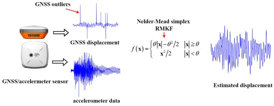
Figure 1.
Nelder-Mead simplex RMKF reduces the impact of GNSS outlier.
Following this introduction, Section 2 provides a systematic review of relevant studies for identifying the knowledge gaps. Section 3 overviews the proposed method. The Nelder-Mead simplex method is combined with MKF to realize GNSS outlier detection and suppress the influence of outliers. Section 4 demonstrates the effectiveness of the proposed method in improving the trustworthiness of BSHM through a field experiment of a suspension bridge. Section 5 includes the conclusion drawn from the above work.
2. Literature Review
2.1. Structural Health Monitoring of Bridges
A linear variable differential transformer (LVDT) is the most reliable and accurate direct displacement measurement sensor with an accuracy of 0.01 mm [3]. Unfortunately, the installation of such fixed contact sensors is an enormously challenging task. For instance, an LVDT can only monitor vertical deflections of bridge decks. Nevertheless, the maintenance of such contact sensors is also challenging. Recently, various non-contact displacement sensors have been favored by practitioners, such as GNSS [4,5], vision sensors [6], LiDAR sensors [7], radar sensors [8], fiber bragg grating (FGB) sensors and contact FBG liquid-level systems [9,10], and MEMS [11]. All such sensors have been developed and widely utilized in the current practice of BSHM.
The high-frequency acceleration observations can be double-integrated to obtain vibration displacements. However, hardware flaws in the accelerometer could cause errors and noise that lead to deviations. Such deviations could accumulate gradually over time which impede effective structural health monitoring (SHM) [12]. Previous studies have developed methods that use short-term zero-mean dynamic displacement for eliminating accelerometer bias. Various accelerometer denoise methods have been proposed, such as baseline correction techniques, high-pass filtering [13], least-squares-based deviation estimation [14], the state-space model method [15], velocity estimation [16], and polynomial data fitting [17]. Nevertheless, these deviations are not constant values since the sensor may be prone to deviation or temperature instability in the long-term observation state. Therefore, it is difficult to accurately monitor the displacement of bridge structure for a long time by only relying on acceleration time-frequency integration. In the current practice, accelerometer is mainly used to measure the local vibration acceleration of the bridge structure rather than to attain long-term dynamic displacement measurements.
GNSS positioning has also been applied to the SHM of long bridges and has gradually become one of the main tools for long-term operation and maintenance monitoring with the advance of GNSS technologies. GNSS BSHM can reflect the dynamic displacement change process of the structure from the independent coordinate system of the bridge. GPS was validated by Ashkenazi et al. (1997) for the feasibility of bridge dynamic monitoring on the Humber Bridge in the UK [18]. It proved that real-time kinematic (RTK) positioning can measure the three-dimensional (3D) dynamic displacement of bridges with an accuracy of up to a few millimeters. Meng et al. (2018) used GNSS to monitor several bridges and established the framework for integrated GNSS and Earth observation for structural health monitoring (GeoSHM) system to monitor the Forth Road Bridge (FRB) in Scotland in real-time [19]. Together with the FRB, two other bridges on the Yangtze River in China were selected as test structures: Wuhu Yangtze Bridge and Ningbo Zhaobaosang Bridge. GNSS technology has been mature in static deformation monitoring technology, but dynamic deformation monitoring is still in the research and development stage. In addition, GNSS outliers exist under a quite hostile observation environment when GNSS signals are either blocked by bridge structure, reflected by the water surface underneath the bridge and by moving vehicles, or even caused by GNSS satellite orbit anomalies. GNSS outliers will cause false alarms, especially in extreme events such as earthquakes and typhoons when timely and reliable operational information of bridges is critical.
Integrated applications of multiple sensors could make full use of their collective advantages for improving the integrity and accuracy of an SHM system. GNSS can easily identify low-frequency components of structural vibration. On the contrary, the accelerometer can easily to detect the high-frequency component of structural vibration. Integrating these two sensors could help remedy their individual drawbacks and enhance the SHM system’s ability to precisely measure the dynamics of a monitored bridge such as vibration frequencies, 3D displacements, etc. Meng et al. (2002) effectively combined GPS and accelerometer to accurately identify the vibration frequencies of bridge structures under different external excitations [20]. They developed a peak-picking algorithm to identify the natural frequency of Wilford Bridge based on GPS and accelerometer measurements. Xiong et al. (2017) analyzed the close relationship between GNSS multipath error and the measurement environment in detail and assessed the noise reduction performance of different filtering algorithms [21]. An autocorrelation function-based empirical Chebyshev (AFEC) hybrid filtering algorithm for integrated monitoring with GNSS and accelerometer is proposed by Xiong, and the results prove that the first five natural frequencies of bridge structures can be accurately identified in a dynamic displacement monitoring environment. The optimal result can be obtained through recursive adjustment of parameters, and post-processing fusion can be realized only when all measurements have been completed, which makes this method unable to be widely applied in actual BSHM. For BSHM, it is essential to continuously assess the integrity and safety of a monitored structure and alert abnormal behavior on time.
The Research and Development (R&D) of real-time Kalman filter is a multi-rate and multi-source data fusion technology that is crucial for conducting an automated diagnosis of bridge structures in BSHM. Kalman filtering explicitly considers the noise in the measurements and minimizes its impact on the decision-making process. Based on the observed displacement and acceleration measurement, Smyth et al. (2007) proposed a MKF and Rauch–Tung–Striebel (RTS) backward smoothing method for the first time [22]. Bock et al. (2011) carried out loosely-coupled integration between GNSS and seismic monitoring data with a 100 Hz accelerometer and achieved a displacement accuracy of 1.6 mm–2.3 mm under favorable conditions [23]. Sara (2017) provided an SHM solution to demonstrate the feasibility of real-time, multi-source sensor fusion monitoring. Fusion results of real-time GNSS and acceleration are obtained with wireless communication transmission methods under laboratory environments but have not been verified extensively in practice [24]. Kogan (2008) realized the fusion of 5 Hz GNSS displacement and 100 Hz acceleration based on the conventional MKF and verified bridge vibration excited by marathon runners, conventional traffic, and air temperature [25]. Yan et al. (2017) demonstrated that the maximum likelihood estimation combined with MKF could be used to fuse GNSS and accelerometer sensor data, and the noise could be effectively mitigated. This method has been verified via numerical simulation and field data and it proves to be able to improve GPS measurement accuracy and expand frequency bandwidth [26]. However, the noise ratio of a multiple sensory system needs to be determined for obtaining optimal estimation results. Cho et al. (2016) proposed an indirect bridge displacement estimation method based on Kalman filtering [27]. This method used non-referential multi-metric response (i.e., acceleration and strain), which was verified by truck tests on a concrete bridge with good calculation effect on the real full-size bridge. Meng et al. (2014) proposed an extended Kalman filter (EKF) based on the 5-dimensional state for GNSS/acceleration vertical data fusion. The feasibility of this method was assessed through simulation experiments and the analysis of the measured data of Wilford Bridge in England [28]. At the same time, the world’s first highly integrated GNSS/accelerometer receiver for bridge monitoring has been developed and used for monitoring the FRB in Scotland [29].
2.2. Outlier Detection
Sensor defects and complex measurement environments affect measurement quality in long-term bridge structural monitoring, and this leads to very often outlier occurrences in measurement data. Coupled with measurement noise or sensor bias, outliers in the measurement data will cause misjudgments of bridge operational status or even lead to false alarms. Firstly, depending on hardware quality and observation environments GNSS measurement noise cannot be fully removed or mitigated, so accurate displacement cannot be obtained even through the fusion of GNSS and accelerometer data. Yang et al. (2021) proposed an adaptive multi-rate RTS smoother to estimate unknown GNSS displacement noise based on the variable decibels Bayesian technique. The displacement accuracy of fused GNSS displacement and acceleration was improved, and the accuracy reached 2.1 mm in the field test experiment [30]. However, this method was only used in a post-processing mode. Niu et al. (2014) proposed an adaptive MKF that combined the Helmert method of variance component with MKF and then simulated in a real-time mode to estimate the process state and process noise variance simultaneously [31]. The limitation of this method was that the GNSS noise to be observed needs to be accurately known and stable for a long time; otherwise, the deviation of GNSS noise observed will be transferred to the accelerometer noise estimation. Secondly, the acceleration bias will destroy the state model in the filter, and also indirectly affect the real-time displacement accuracy. Kim et al. (2018) introduced a simplified two-stages Kalman filter (TSKF) method, aiming at the data fusion of GNSS RTK and acceleration [9]. The acceleration bias was estimated via two-stage filtering updates and verified with simulation and through measured vibration tests. Whereas, this method is only applicable when there are no outliers in the measurements. Thirdly, outliers may affect the accurate modal identification or structural damage detection in an SHM system. The caveat is that outliers may be caused by real structural damages or simply due to sensor anomaly. Su et al. (2022) proposed a state-domain robust autonomous integrity monitoring algorithm based on extrapolation to identify slow-growing gross errors of GNSS/accelerometers in a BSHM system [29]. Whereas this method can detect gross errors, it cannot be used to eliminate gross errors. Jing et al. (2022) used the anomaly observation variance expansion model to process the simulated landslide monitoring data (raw GNSS and acceleration) in three typical scenarios: normal locking of GNSS signal, partial loss of signal, and short-term interruption [32]. It was verified that GNSS/accelerometer integration can effectively identify the real state of the landslide, but it did not take into account the large attitude drift caused by the accelerometer in the actual landslide. To sum up, previous studies for eliminating the influence of GNSS outlier data have the defects of only implementing post-processing or recursive adjustment, which makes it difficult to accurately estimate the optimal displacement in real-time.
Huge amounts of GNSS outliers often occur in BSHM measurements due to atmospheric conditions, multipath effects, signal obstruction, and satellite geometry. False alarms could be easily triggered in the BSHM system. This study proposed an RMKF based on Nelder-Mead simplex optimal estimation to mitigate the influence of the GNSS observation outliers on the state parameters. First, MKF is constructed as a weighted least squares model. Then a residual model is developed. Finally, the optimal robust estimation solution of the Nelder-Mead simplex method is realized. The proposed method solves the abnormal defects of GNSS observation in real-time multi-source data fusion in BSHM and proves to have good applicability in bridge monitoring.
3. Methodology
Figure 2 shows a flowchart that contains the major steps of the proposed method. Firstly, the state model and measurement model of GNSS/acceleration are constructed. Secondly, the above model is modified into the least squares model (LSM). Thirdly, an optimal estimation algorithm based on the Nelder-Mead simplex method is proposed and applied to the least squares model to achieve the filtered optimal estimation. Finally, the anomaly of GNSS can be fully detected and their influence can be reduced to improve the credibility of BSHM.
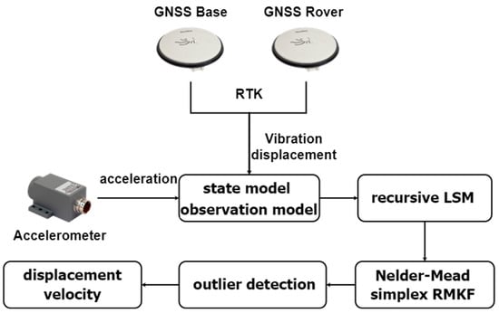
Figure 2.
A flowchart of the proposed method.
3.1. MKF Model Based on GNSS/Acceleration
The displacement with GNSS positioning is taken as the measurement of correction in the MKF, and the acceleration as the control quantity of the MKF prediction model. The MKF method of the constant acceleration model is adopted. The data fusion of low sampling rate displacement and high sampling rate acceleration is realized [22], and its dynamic discretization prediction model is as follows:
In this equation, indicates the displacement and velocity status parameter of the system at time , represents the state one-step prediction matrix at time , represents the transfer matrix of acceleration at time ; illustrates the acceleration information at time ; and is the time between the actual accelerometer acquisition. represents the system noise distribution matrix. indicates the system noise vector. The system state noise can be expressed as:
where is the random walk parameter of the accelerometer. The low-frequency GNSS displacement obtained from the monitoring of the bridge structure is taken as the measurement information to construct the discrete observation model:
where illustrates the three-dimensional GNSS displacement at time , corresponding to the longitudinal (defined as along the bridge main axis), lateral (vertical to the bridge main axis), and vertical directions of the bridge structure respectively; represents the design matrix of the measurement equation at time ; indicates the noise vector of the observation equation at time ; indicates the design matrix of the observation equation at time , whose internal components have non-correlation; represents the variance of GNSS displacement at time ; and represents GNSS displacement sampling frequency. The above system model can be expressed by traditional discrete linear filtering, and the process is as follows:
and represent a state linear one-step prediction and its mean square error matrix, respectively. is the filter gain matrix. and represent the state estimation and its mean square error matrix at time k.
The parameter estimation process of the Kalman filter can also be considered as the solution of a specific weighted least squares, and the state prediction model Equation (1) and observation model Equation (4) are transformed into:
The stochastic model is a block diagonal cofactor matrix and the Cholesky decomposition is performed to attain:
Multiply Equation (8) by to get:
Therefore, Equation (11) is a standard least squares regression problem form, which can produce the optimal estimate:
It is proved that Equation (7) of the recursive procedure of Kalman filtering is consistent with the linear optimal solution provided by Equation (12). However, if abnormal measurements are introduced into the system, the filter will appear unstable. For example, if the GNSS receiver is malfunctioning due to long-term operation, resulting in outliers in the BSHM system. Additionally, when satellite geometries are poor or multipath effects occur due to water fluctuation and vehicle dynamic reflection, the precision of the GNSS displacement decreases, resulting in outliers of the data. GNSS signals are blocked by bridge elements because the actual bridge operation and maintenance environment are very complex and changing. As a result, the cycle slip of GNSS is a very common situation in BSHM. Shown in Figure 3 are the 3D real-time GNSS displacements of the SHM8 and SHM9 monitoring points at the quarter-span positions of the FRB on 1 September 2019. Outliers in the SHM8 displacement time series appeared for about five seconds, while SHM9 located on the other side of the quarter span showed no abnormal displacement. However, it was only the GNSS cycle slips that caused outliers at the SHM8. If the robustness of the SHM system is also poor, it will introduce further measurement outliers, often producing false alarms, so an effective real-time robust filter is critical for a reliable BSHM system.
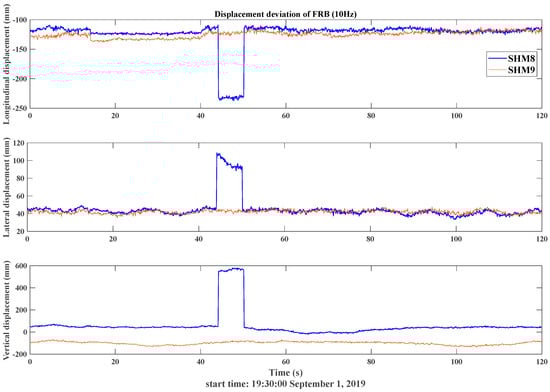
Figure 3.
The GNSS cycle slips caused abnormal displacements in the FRB. The upper row shows the results of longitudinal displacements, the middle row the results of lateral displacements, and the bottom row the results of vertical displacements, respectively.
3.2. Optimal Robust Estimation Method Based on Nelde-Mead
The Kalman filter is a tool for resolving a linear regression problem. However, it is necessary to develop a robust optimal method because of the existence of outliers in the actual system. Firstly, the residual error model of measurement information and state estimation is constructed.
where is the row vector ; is the row vector of ; is the matrix dimension; represents a residual model for anomaly observation, and its random error is the Gaussian normal distribution. However, due to the existence of measurement outliers, the noise of the actual residual model does not obey the Gaussian normal distribution. Therefore, the authors adopted a residual estimation model, i.e., the Huber model, which is sensitive to outliers in this study.
In the formula, the experience threshold is set to 1.5. In this manuscript, the Nelde-Mead simplex optimal estimation method is used to estimate the minimum residual in real-time. Nelder and Mead designed new steps such as extension and compression on the normal simplex method and made it an arbitrary simplex. It is called the Nelder-Mead simplex algorithm to make it an effective optimization search method [33]. The Nelder-Mead simplex algorithm is a search algorithm for solving multi-parameter optimization problems, which has certain advantages in solving multi-variable function minimization problems. The Nelder-Mead simplex has a strong local search ability and does not require the permeability of the objective function. The simplified model form in the residual model is
where is called an influence function of mode . The Nelder-Mead simplex is a dimensional geometric figure, which is a convex hull made up of vertices denoted by . The method iteratively generates a sequence of simple forms that approximates the optimal estimate . In each iteration, the simplex vertices are ordered according to the value of the objective function
where is the optimal vertex and is the worst vertex. The Nelder-Mead simplex method uses four possible operations, each associated with a scalar parameter: (reflection), (expansion), (contraction), and (shrink). The values of these parameters satisfy , , , and . These parameter criteria are selected as
Let be the center of mass of optimal vertices, expressed as
The above is the idea of Nelder-Mead’s method, and one detailed iteration is:
- Step 1: Firstly, vertices are sorted in the form of an Equation (17).
- Step 2: Reflection point :and evaluate . If , replace with .
- Step 3: If , compute the expansion point :and evaluate . If , replace with , otherwise .
- Step 4: If , compute the outside contraction point :and evaluate . If , replace with , otherwise jump directly into step 6.
- Step 5: If , compute the inside contraction point :
- Step 6: For , define:
According to the Nelder-Mead simplex method above, the optimal estimation can be achieved, and the overall flow chart of the method in this manuscript is given in Figure 4.
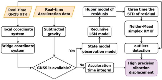
Figure 4.
Flow chart of GNSS/accelerometer integrated bridge structural health monitoring based on Nelder-Mead Simplex tolerance.
4. Case Study—SHM of the Wilford Suspension Bridge
The effectiveness and reliability of the proposed method are verified by a field BSHM test. First, the authors introduced the location of the experiment and the sensors of this experiment. It verified that the low-cost GNSS receiver with an accelerometer can meet the high precision of bridge structural health monitoring. Secondly, this experiment was a field experiment, which does not have the reference results as in laboratory conditions. A simple and desirable method was used to obtain the high-precision vibration displacement of the bridge. Finally, through the simulated real-time GNSS and acceleration data fusion method, it is verified that the proposed method is conducive to reducing the influence of GNSS outliers and improving the credibility of BSHM.
4.1. Experiment Setup
The Wilford Suspension Bridge is a double-main cable gravity-anchored footbridge over the River Trent in Nottinghamshire, England. With a span of 69 m and a width of 3.7 m, the bridge is mainly used for residents on both sides of the river and for carrying water pipes and it is composed of a steel deck covered by a floor of wooden slats, as shown in Figure 5. The University of Nottingham has carried out several bridge structural health monitoring tests on the bridge because of its large deflections (decimeter range) under normal environmental loading. Fine finite element (FFE) analysis was carried out using the field measurement of the bridge structure size and materials [20]. The FFE model can obtain the first three natural frequencies of the Welford Bridge, which provides a reliable and comprehensive reference for adopting the proposed method.
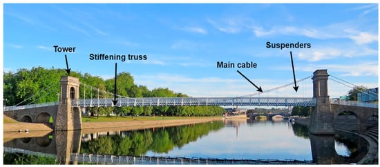
Figure 5.
Wilford Suspension Bridge in England.
The authors carried out field tests on the suspension bridge from 15:48 to 16:30 on 31 October 2018. Two types of GNSS receivers were used in this experiment for data collection: (1) Leica GS10 GNSS geodesic receivers, whose raw observations can be sampled at a frequency of 20 Hz. It can be realized by RTK technology, horizontal 8 mm + 1 ppm, vertical 15 mm + 1 ppm, and accuracy confidence reaches more than 99.99%. (2) DM3 geodesic GNSS receivers that were manufactured by the GeoSHM team [16], as shown in Figure 6. These receivers, as the first of their type, are also equipped with low-cost and high-precision MEMS accelerometers. The acquisition frequency of GNSS raw observations in both receivers is 20 Hz. The collected data of DM3 can obtain the same positioning accuracy and confidence interval as Leica GS10 GNSS geodesic receivers by post-processing kinematic (PPK). The sampling frequency of the accelerometer in the DM3 receiver is 100 Hz, the range is 2 g, and the acceleration noise spectrum is . In addition, supporting GNSS signal splitters, power supply, and so on are also essential.
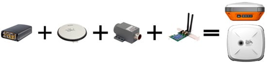
Figure 6.
DM3 geodesic GNSS/accelerometer receivers that were manufactured by the GeoSHM team. The sensor integrates a GNSS receiver, GNSS antenna, accelerometer and real-time wireless module.
During field tests, two pairs of GS10 and DM3 receivers were placed in the quarter span and the middle span of the suspension bridge, respectively. In this experiment, the measurement information of a DM3 receiver installed in the middle position was analyzed and verified the measurement of the vibration displacement of footbridges in Nottingham (Figure 7). Another GS10 receiver is used as a reference station around 100 m away from the monitoring points, as shown in Figure 7a. The dynamic vibration of the bridge is caused by the forced vibration combined with the random vibration due to wind loading. In addition, Figure 8 shows that the power spectral densities (PSD) extracted from the GNSS measurements of both types of receivers in the three directions are very similar, indicating that the low-cost receiver fully meets the accuracy requirements of bridge structure monitoring. Therefore, in the subsequent experiments of this section, data collected with a DM3 receiver is used for analysis.
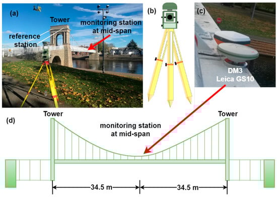
Figure 7.
The Wilford Suspension Bridge in Nottingham and the instrumentation. (a) Actual locations of monitoring and reference stations; (b) reference station; (c) monitoring station (DM3 and Leica GS10) (d) the monitoring devices were fixed at the mid-span of the footbridge for dynamic response monitoring.
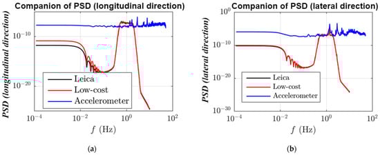
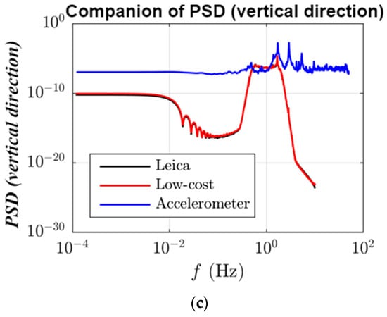
Figure 8.
The power spectral densities (PSD) are identified by the Leica receiver (black), self-developed receiver (DM3 red), and accelerometer measurements (blue). The top left row (a) shows the PSD of longitudinal direction measurements and the top right row (b) shows the PSD of lateral direction measurements and the bottom (c) shows the PSD of vertical direction measurements.
4.2. Pretreatment
The data collected by GNSS and accelerometer using different coordinate systems need to be registered. The WGS84 geodetic coordinate system is used for GNSS and the accelerometer is used for the local bridge coordinate system. The WGS84 system coordinates need to be converted to the British OSGB 36NG coordinate system through the OSGM15 model. The coordinates are then converted to the bridge coordinate system by the method of plane rotation.
The displacement of the bridge is small and irregular due to the influence of its gravity and the underneath water pile loading. In addition, the multipath error is one of the unavoidable error sources of BSHM, which is difficult to eliminate or weaken by the empirical model or GNSS RTK. These combined effects will obscure the dynamic vibration component in the GNSS displacement time series. To reduce the interference caused by the special environment, this manuscript uses the Butterworth high-pass filter to eliminate the long-term slow displacement changes existing in the GNSS displacement time series, as shown in Figure 9.

Figure 9.
GNSS displacement and dynamic vibration displacement after Butterworth at the mid−span of the Wilford Suspension Bridge. The upper row shows the results of longitudinal displacements, the middle row shows the results of lateral displacements and the bottom row shows the results of vertical displacements.
The double integral of acceleration is taken as the reference displacement. Firstly, due to the hardware delay of the data acquisition system, some epoch data are lost. The Lagrange interpolation method was used to fit the missing original acceleration data first. Secondly, the triaxial acceleration data are processed by a fifth-order Butterworth high-pass filter with a bandpass frequency of 0.2 Hz. Finally, the dynamic displacement of the bridge was obtained by time domain integration. As shown in Figure 10, the monitoring time series results of the longitudinal (along), lateral (across), and vertical axes of the bridge are respectively represented, and the results are taken as the reference truth value of this test. However, the acceleration data in the GNSS/accelerometer fusion is the original observational data that has not been processed with the Butterworth filter.
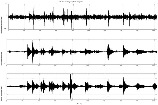
Figure 10.
Displacement time series through acceleration time-frequency integration. The upper row shows the results of longitudinal displacements, the middle row shows the results of lateral displacements and the bottom row shows the results of vertical displacements.
The dynamic response of the bridge structure in the three directions can be seen from the integral result of acceleration. There is no obvious vibration and displacement deformation in the longitudinal direction, but there are apparent dynamic responses caused by forced movements in the lateral and vertical directions.
4.3. Robust Kalman Test for Detecting the Random Outliers of GNSS
This section verifies the reliability and accuracy of the proposed method in GNSS outliers data detection. The random errors were obtained using a Gaussian-based random method with a range of (−20 mm–20 mm). These errors were then added to 1% of the time series of three-dimensional displacements. The histograms of random errors of dynamic displacements in three different directions are shown in Figure 11. The displacement has many outliers, making the distribution wider. This step is used to represent the simulation method of random outliers in GNSS displacement caused by changes in the external environment or abnormal hardware equipment. This section only shows the analysis results of part of the data from 200 s to 500 s to show the feasibility of the algorithm more clearly.
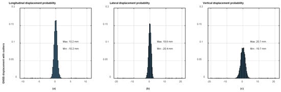
Figure 11.
Histograms of random errors of dynamic displacements in three different directions. The left row (a) shows the errors of longitudinal displacements, the intermediate row (b) shows the results of lateral displacements and the right row (c) shows the results of vertical displacements.
In Figure 12, 3D displacements are represented as high-precision double integral displacement of acceleration (blue), GNSS/acceleration fusion results based on the MKF method (red), and GNSS/acceleration fusion results based on the Nelder-Mead simplex RMKF (black). The RMKF method has improved both RMS, Min and Max of error combined with Table 1. The total displacement accuracy of the RMSE value has been improved by 21%. For abnormal error values, Nelder-Mead simplex RMKF has a better effect of suppressing the influence of GNSS outliers than MKF.
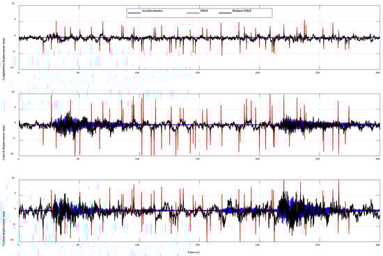
Figure 12.
Dynamic displacements obtained in three different directions from the double integral of acceleration (blue), GNSS and accelerometer data fusion with MKF method (red), and GNSS and accelerometer data fusion with the proposed RMKF method (black). The upper row shows the results of longitudinal displacements, the middle row shows the results of lateral displacements and the bottom row shows the results of vertical displacements.

Table 1.
Comparison table Mean, RMS, Max and Min error of the MKF and Robust MKF based on data of longitudinal, lateral, vertical, and total displacement.
The PSD signatures of the acceleration double integration, GNSS displacements, and displacements estimated from fusing the GNSS and accelerometer data with the proposed robust RMKF method were analyzed based on the fast fourier transform (FFT) and shown in Figure 13. At the same time, it can be seen from Figure 10 above that the bridge structure has no obvious vibration in the longitudinal direction, so this manuscript only focuses on representative PSD patterns in the lateral and vertical directions.
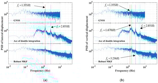
Figure 13.
Power spectral densities (PSD) of displacements from GNSS data (upper row), accelerometer measurements (middle row), and displacements from GNSS and accelerometer data fusion with the proposed RMKF method (bottom row). The left row (a) shows the results of lateral displacements and the right row (b) shows the results of vertical displacements.
Firstly, Figure 13a shows that the first mode natural frequency of 1.355 Hz and the third natural frequency of 2.855 Hz in the GNSS displacement value can be recognized, but the second mode frequency is not clear. The authors fused GNSS and acceleration data with the RMKF method to extract the second natural frequency. Figure 13b shows that GNSS data in the vertical direction did not identify the first natural frequency of 1.355 Hz because the energy of this frequency was lower than that of the second natural frequency of 1.670 Hz. For the natural frequency of 5.236 Hz, GNSS data cannot be identified. Theoretically, the sampling rate of 20 Hz of GNSS data may detect signals up to 10 Hz. However, due to the noise and outliers existing in the data during the actual observation, the modal frequency of 5.236 Hz has been buried in it, and it cannot be identified through spectral analysis. In contrast, the accelerometer data and the combination of GNSS and accelerometer data capture the frequency well.
The advantage of the RMKF is also demonstrated by comparing alarm thresholds. During the field experimenters, a large number of jumping or running situations were executed, resulting in large dynamic vibration of the bridge in the experiment. Therefore, it is unscientific to use a fixed threshold to monitor the displacement and to give an alarm when the threshold is exceeded. The alarm threshold interval is mainly divided into three steps. First, the double integral dynamic displacement of the accelerometer with noise reduction is used as a reference. Then the error-free GNSS/acceleration fusion displacement is distinguished from the reference. Finally, three times the standard deviations (STD) are constructed as the threshold range, as shown in Figure 14. If the residual difference between the obtained displacement and the reference value exceeds the threshold range, it is judged as an alarm situation. After Nelder-Mead simplex RMKF treatment, the influence of GNSS outliers is effectively weakened, so that their displacement is below the threshold, and there is no error alarm. However, the displacements (with many blue spikes) processed by conventional MKF still exceed the threshold, which will affect the assessment of structural conditions, and in this case, the false alarm rate reaches 92%. Therefore, the RMKF method can effectively improve the accuracy of the alarm system and greatly reduce the false alarm caused by these gross errors.
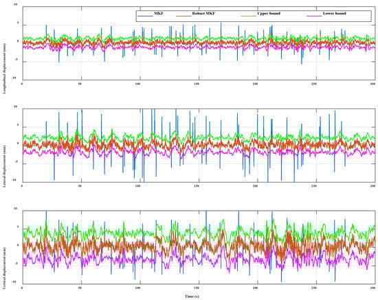
Figure 14.
Spatiotemporal warning of dynamic displacement error. The upper row shows the results of l longitudinal displacements, the middle row shows the results of lateral displacements and the bottom row shows the results of vertical displacements.
5. Conclusions
In this study, the authors have developed an anomaly-detection method based on RMKF to better realize the integrated monitoring of bridges with GNSS and acceleration. The proposed method estimates each epoch fusion result and mitigates the time impacts of GNSS observed outliers in real-time. The results from the case studied bridge indicate that the proposed method has good performance in reducing the effect of GNSS outliers. Besides, the proposed method can make better use of the complementary properties of GNSS and acceleration data and overcome the shortcomings of GNSS-based technology for BSHM. Limitations of the proposed method still exist. For example, the proposed method could only be used for detecting outliers of a single sensor. In the future, the authors are committed to combining a priori information to realize the short-term and high-precision monitoring of bridge structure status even when multi-sensors bear outliers. In addition to the normal environmental monitoring of bridge operation and maintenance, monitoring in the special harsh environment is more important. Therefore, the follow-up of this study aims to accurately identify whether the abnormal observation in a naturally harsh environment is due to the abnormal structure of the bridge or the abnormal phenomenon of sensor data. Meanwhile, based on GNSS technology, the BSHM system of multi-sensor observation is constructed to realize the mutual evaluation of multi-source data and realize the high-precision and reliability decision of infrastructure.
Author Contributions
Conceptualization, L.H. and X.M.; methodology, L.H.; software, L.H.; validation, L.H.; formal analysis, L.H.; investigation, L.H.; resources, Y.B.; data curation, Z.S., C.T. and D.Z.; writing—original draft preparation, L.H.; writing—review and editing, X.M., Z.S. and Y.B.; visualization, X.M.; supervision, X.M.; project administration, L.H. and X.M.; funding acquisition, L.H. and X.M. All authors have read and agreed to the published version of the manuscript.
Funding
This research was funded by the National Natural Science Foundation of China (grant No. 51829801) and the Collaborative Innovation Project of Chaoyang District, Beijing (grant No. CYXC2207).
Data Availability Statement
Data available on request due to restrictions eg privacy or ethical The data presented in this study are available on request from the corresponding author.
Acknowledgments
The first author would like to thank Yilin Xie and George Ye for providing the experimental data gathered from a UK bridge supported by the European Space Agency and other UK national funding bodies.
Conflicts of Interest
The authors declare no conflict of interest.
Abbreviations
| GNSS | Global Navigation Satellite Systems |
| BSHM | Bridge Structural Health Monitoring |
| LVDT | Linear variable differential transformer |
| SHM | Structural Health Monitoring |
| RTK | Real-time Kinematic |
| AFEC | Autocorrelation Function-based Empirical Chebyshev |
| MKF | Multi-rate Kalman Filter |
| RTS | Rauch–Tung–Striebel |
| EKF | Extended Kalman Filter |
| TSKF | Two Stages Kalman Filter |
| RMKF | Robust Multi-rate Kalman Filter |
| GeoSHM | GNSS and Earth Observation for Structural Health Monitoring |
| FRB | Forth Road Bridge |
| FFE | Fine Finite Element |
| PSD | Power Spectral Densities |
| FFT | Fast Fourier Transform |
References
- Report Card For America’s Infrastructure. 2021. Available online: https://infrastructurereportcard.org/cat-item/bridges-infrastructure/ (accessed on 1 April 2023).
- Haldar, A. Health Assessment of Engineered Structures; World Scientific: Singapore, 2012. [Google Scholar] [CrossRef]
- Hidayat, I.; Suangga, M.; Maulana, M.R. The effect of load position to the accuracy of deflection measured with LVDT sensor in I-girder bridge. IOP Conf. Ser. Earth Environ. Sci. 2017, 109, 12–24. [Google Scholar] [CrossRef]
- Yu, J.; Meng, X.; Yan, B.; Xu, B.; Fan, Q.; Xie, Y. Global Navigation Satellite System-based positioning technology for structural health monitoring: A review. Struct. Control Health Monit. 2019, 27, e2467. [Google Scholar] [CrossRef]
- Ge, Y.; Cao, X.; Lyu, D.; Zaimin, H.; Ye, F.; Xiao, G.; Shen, F. An investigation of PPP time transfer via BDS-3 PPP-B2b service. GPS Solut. 2023, 27, 61. [Google Scholar] [CrossRef]
- Yu, S.; Xu, Z.; Su, Z.; Zhang, J. Two flexible vision-based methods for remote deflection monitoring of a long-span bridge. Measurement 2021, 181, 109658. [Google Scholar] [CrossRef]
- Xiao, Q.; Liu, Y.; Zhou, L.; Liu, Z.; Jiang, Z.; Tang, L. Reliability analysis of bridge girders based on regular vine Gaussian copula model and monitored data. Structures 2022, 39, 1063–1073. [Google Scholar] [CrossRef]
- Kilic, G.; Unluturk, M.S. Wavelet Analysis with Different Frequency GPR Antennas for Bridge Health Assessment. J. Test. Eval. 2016, 44, 647–655. [Google Scholar] [CrossRef]
- Alamandala, S.; Prasad, R.; Pancharathi, R.K.; Pavan, V.D.R.; Kishore, P. Study on bridge weigh in motion (BWIM) system for measuring the vehicle parameters based on strain measurement using FBG sensors. Opt. Fiber Technol. 2021, 61, 102440. [Google Scholar] [CrossRef]
- Bonopera, M.; Chang, K.-C.; Chen, C.-C.; Lee, Z.-K.; Sung, Y.-C.; Tullini, N. Fiber Bragg Grating—Differential Settlement Measurement System for Bridge Displacement Monitoring: Case Study. J. Bridge Eng. 2019, 24, 05019011. [Google Scholar] [CrossRef]
- Khodabandehlou, H.; Pekcan, G.; Fadali, M.S. Vibration-based structural condition assessment using convolution neural networks. Struct. Control Health Monit. 2019, 26, e2308. [Google Scholar] [CrossRef]
- Sohn, H.; Kim, K.; Choi, J.; Koo, G.; Chung, J. Development of a High Accuracy and High Sampling Rate Displacement Sensor for Civil Engineering Structures Monitoring. In Experimental Vibration Analysis for Civil Structures; Springer International Publishing: Berlin/Heidelberg, Germany, 2018; pp. 62–70. [Google Scholar]
- Trifunac, M.D. Zero baseline correction of strong-motion accelerograms. Bull. Seismol. Soc. Am. 1971, 61, 1201–1211. [Google Scholar] [CrossRef]
- Chiu, H.-C. Stable baseline correction of digital strong-motion data. Bull. Seismol. Soc. Am. 1997, 87, 932–944. [Google Scholar] [CrossRef]
- Gindy, M.; Vaccaro, R.; Nassif, H.; Velde, J. A State-Space Approach for Deriving Bridge Displacement from Acceleration. Comput.-Aided Civ. Infrastruct. Eng. 2008, 23, 281–290. [Google Scholar] [CrossRef]
- Park, K.-T.; Kim, S.-H.; Park, H.-S.; Lee, K.-W. The determination of bridge displacement using measured acceleration. Eng. Struct. 2005, 27, 371–378. [Google Scholar] [CrossRef]
- Zhu, L. Recovering permanent displacements from seismic records of the June 9, 1994 Bolivia deep earthquake. Geophys. Res. Lett. 2003, 30, 1700–1704. [Google Scholar] [CrossRef]
- Ashkenazi, V.; Roberts, G.W. Experimental monitoring of the Humber Bridge using GPS. ICE Proc. Civ. Eng. 1997, 120, 177–182. [Google Scholar] [CrossRef]
- Meng, X.; Nguyen, D.T.; Xie, Y.; Owen, J.; Psimoulis, P.; Ince, S.; Chen, Q.; Ye, J.; Bhatia, P. Design and Implementation of a New System for Large Bridge Monitoring—GeoSHM. Sensors 2018, 18, 775. [Google Scholar] [CrossRef]
- Xiaolin, M. Real-Time Deformation Monitoring of Bridges Using GPS Accelerometers. Ph.D. Thesis, University of Nottingham, Nottingham, UK, 2002. [Google Scholar]
- Xiong, C.; Lu, H.; Zhu, J. Operational Modal Analysis of Bridge Structures with Data from GNSS/Accelerometer Measurements. Sensors 2017, 17, 436. [Google Scholar] [CrossRef]
- Smyth, A.; Wu, M. Multi-rate Kalman filtering for the data fusion of displacement and acceleration response measurements in dynamic system monitoring. Mech. Syst. Signal Process. 2007, 21, 706–723. [Google Scholar] [CrossRef]
- Bock, Y.; Melgar, D.; Crowell, B.W. Real-Time Strong-Motion Broadband Displacements from Collocated GPS and Accelerometers. Bull. Seismol. Soc. Am. 2011, 101, 2904–2925. [Google Scholar] [CrossRef]
- Casciati, S.; Vece, M. Real-time monitoring system for local storage and data transmission by remote control. Adv. Eng. Softw. 2017, 112, 46–53. [Google Scholar] [CrossRef]
- Kogan, M.G.; Kim, W.-Y.; Bock, Y.; Smyth, A.W. Load Response on a Large Suspension Bridge during the NYC Marathon Revealed by GPS and Accelerometers. Seismol. Res. Lett. 2008, 79, 12–19. [Google Scholar] [CrossRef]
- Yan, X.; Brownjohn, J.M.W.; David, H.; Young, K.K. Long-span bridges: Enhanced data fusion of GPS displacement and deck accelerations. Eng. Struct. 2017, 147, 639–651. [Google Scholar] [CrossRef]
- Cho, S.; Park, J.-W.; Palanisamy, R.P.; Sim, S.-H. Reference-Free Displacement Estimation of Bridges Using Kalman Filter-Based Multimetric Data Fusion. J. Sens. 2016, 2016, 3791856. [Google Scholar] [CrossRef]
- Meng, X.; Wang, J.; Han, H. Optimal GPS/accelerometer integration algorithm for monitoring the vertical structural dynamics. J. Appl. Geod. 2014, 8, 265–272. [Google Scholar] [CrossRef]
- Sun, A.; Zhang, Q.; Yu, Z.; Meng, X.; Liu, X.; Zhang, Y.; Xie, Y. A Novel Slow-Growing Gross Error Detection Method for GNSS/Accelerometer Integrated Deformation Monitoring Based on State Domain Consistency Theory. Remote Sens. 2022, 14, 4758. [Google Scholar] [CrossRef]
- Yang, A.; Wang, P.; Yang, H. Bridge Dynamic Displacement Monitoring Using Adaptive Data Fusion of GNSS and Accelerometer Measurements. IEEE Sens. J. 2021, 21, 24359–24370. [Google Scholar] [CrossRef]
- Niu, J.; Xu, C. Real-Time Assessment of the Broadband Coseismic Deformation of the 2011 Tohoku-Oki Earthquake Using an Adaptive Kalman Filter. Seismol. Res. Lett. 2014, 85, 836–843. [Google Scholar] [CrossRef]
- Jing, C.; Huang, G.; Zhang, Q.; Li, X.; Bai, Z.; Du, Y. GNSS/Accelerometer Adaptive Coupled Landslide Deformation Monitoring Technology. Remote Sens. 2022, 14, 3537. [Google Scholar] [CrossRef]
- Gao, F.; Han, L. Implementing the Nelder-Mead simplex algorithm with adaptive parameters. Comput. Optim. Appl. 2010, 51, 259–277. [Google Scholar] [CrossRef]


Disclaimer/Publisher’s Note: The statements, opinions and data contained in all publications are solely those of the individual author(s) and contributor(s) and not of MDPI and/or the editor(s). MDPI and/or the editor(s) disclaim responsibility for any injury to people or property resulting from any ideas, methods, instructions or products referred to in the content. |
© 2023 by the authors. Licensee MDPI, Basel, Switzerland. This article is an open access article distributed under the terms and conditions of the Creative Commons Attribution (CC BY) license (https://creativecommons.org/licenses/by/4.0/).