Multi-Constrained Seismic Multi-Parameter Full Waveform Inversion Based on Projected Quasi-Newton Algorithm

Abstract

The multi-parameter full waveform inversion (FWI) that integrates velocity and density can make full use of the kinematic and dynamic information of the measured data to reconstruct the underground model. However, it faces problems of crosstalk between multiple parameters and strong nonlinearity. This research proposes a multi-constrained, multi-parameter FWI framework based on the projected quasi-Newton algorithm. This framework can introduce multiple types of prior geological information, which can effectively improve the problem of multi-parameter inversion. Additionally, the quasi-Newton method can eliminate the crosstalk phenomenon to further improve the inversion convergence speed. Taking the 1994BP model as an example, the results show that the projected quasi-Newton method has a faster convergence speed than the spectral projected gradient method, and reduces the crosstalk between parameters; multiple constraint sets are uniquely projected onto the intersection to ensure that the estimated values of model parameters meet multiple constraints. We also experiment with the overthrust model, which shows that the framework we proposed can improve the inversion accuracy and has good adaptability. The proposed multi-parameter inversion framework can be compatible with more prior information to obtain an inversion model that conforms to geological understanding and shows great potential in seismic exploration.

1. Introduction

The core idea of full waveform inversion (FWI) is to extract geophysical parameters of underground media by establishing an objective function and using the optimization methods to minimize the difference between simulated and observed data [1,2,3]. Seismic wave velocity and medium density are important for the lithology interpretation and reservoir description [4,5]. To obtain as many geophysical parameters of underground media as possible, multi-parameter FWI has become an urgent need [6,7,8]. Multi-parameter FWI is a highly nonlinear and ill-posed problem, which is prone to local minimums [9]. At the same time, many degrees of freedom are introduced into the model space, resulting in crosstalk and trade-offs between different parameters [10,11]. Therefore, reducing the ill-posedness and solving the crosstalk between parameters is the key to realizing the high-accuracy, multi-parameter FWI.

To reduce the ill-posedness of the multi-parameter FWI, one of the optimal solutions is to introduce regularization terms constrained by the prior model. One of the mature regularization methods is to add penalty terms to the objective function [12]. Ref. [13] added a first-order Tikhonov regularization term and a prior model norm term to the objective function as a smoothing operator, and prior information, respectively, to realize the regularization of the inversion problem. Ref. [14] developed an inversion method using a total generalized p-variation regularization scheme, and numerical experiments showed that stratigraphic interfaces and smooth background can be recovered simultaneously. Ref. [15] proposed a minmax-concave total variation (TV) regularization strategy to avoid crosstalk noise and improve the accuracy of multi-parameter inversion. Ref. [16] applied a compound regularization of FWI based on Tikhonov and TV regularization to the wavefield reconstruction inversion and achieved good inversion results. Ref. [17] added a TV regularization term by considering the sparsity of high-order operators, which can effectively identify the layer boundaries. Based on a rough estimate of the subsurface image, Ref. [18] proposed the directional TV (DTV). On one hand, traditional regularization methods usually target one or two regularization terms and lack the application of multiple regularization terms; on the other hand, traditional penalty terms tend to spread deviations concerning a reference model evenly [13], so it is difficult to establish a suitable initial model and control the local value [19]. Furthermore, penalty regularization parameters need to be selected [20]. Therefore, the traditional methods of adding the penalty terms to the objective function need to be improved.

The constrained optimization algorithm which is based on multiple convex sets can overcome the limitations of the conventional regularization method, and can minimize the data misfit function while ensuring the estimated model parameters meet the introduced constraints [21]. The projected gradient method is a powerful tool for solving constrained convex optimization problems. It uses first-order partial differential information, combines multiple constrained projection and nonlinear optimization [22], minimizes the differential function on closed convex sets, and avoids the problem of regularization parameter adjustment. It has been widely studied [23,24] and is well applied in multiple constrained optimization problems [25]. The most commonly used projected gradient method is currently the spectral projected gradient (SPG) algorithm. Ref. [26] applied the SPG algorithm to the single-parameter inversion of the acoustic wave equation in the frequency domain, and successfully solved the multi-constrained FWI problem. However, a serious defect of the SPG algorithm is that the update direction is the negative gradient direction and the convergence speed is slow. Although, it has shown good performance in single-parameter FWI;, but its application in a multi-parameter FWI remains to be tested.

The multi-parameter FWI problem is often abstracted as a quadratic optimization problem in mathematics, which can be divided into the gradient type solution and Newton type solution from an optimization perspective. To improve the convergence of the multi-parameter FWI, ref. [27] used the cross-gradient method to perform the multi-parameter inversion of the variable-density acoustic wave equation, and ref. [28] adopted the truncated Gauss–Newton method to reconstruct velocity and density simultaneously. In the FWI of velocity and density, density has the same radiation pattern as velocity at small and medium angles, and they are coupled together in the short offset data [29]. Considering that the non-diagonal block elements of the approximate Hessian matrix reflect the coupling effect between different parameters, the inverse of the approximate Hessian matrix can eliminate the influence between different parameters [30,31,32]. At the same time, compared with the first-order solution, the second-order solution utilizes the information of the Hessian matrix and has a faster convergence speed in theory.

Therefore, the Newton type projection method is a better choice for the multi-parameter FWI under multiple constraints. The projected quasi-newton (PQN) algorithm is one of the commonly used Newton type projection methods. The PQN algorithm combines the projection algorithm with the quasi-newton algorithm and can effectively use the second-order partial derivative information: Ref. [33] verified that the PQN algorithm is superior to gradient type projection algorithms in terms of computational accuracy; Ref. [34] applied the PQN algorithm to boundary constrained optimization problem; Ref. [35] verified the convergence of the PQN algorithm and confirmed that it can be applied to boundary constrained and simplex problems; and Ref. [36] used the PQN algorithm to achieve nonlinear inversion under simple constraints.

To achieve high-efficiency and high-precision of the seismic multi-parameter FWI, we propose a multi-constrained strategy based on the PQN algorithm. Firstly, the multi- constrained strategy based on the projection method is used to convert geological information into corresponding constraint sets, in order to regularize the inversion problem. Secondly, the PQN algorithm is adopted to compute the projection of variables onto the intersection of constraint sets to ensure that the model parameter estimation meets multiple constraints while objective function is minimized; then, the Limited-memory Broyden–Fletcher–Goldfarb–Shanno (L-BFGS) method [37,38] is used for nonlinear optimization. The pseudo-Hessian matrix is calculated by saving partial gradient operators and model modification, which greatly reduces the storage and computation, and improves the convergence speed of the objective function. Finally, the time-domain multiscale FWI strategy [39,40] is introduced to search for global extremum, gradually. It can mitigate the nonlinearity and further improve the inversion accuracy of velocity and density in the multi-parameter FWI.

The organization of this research is as follows: firstly, we introduce the multi-parameter FWI problem of the variable density acoustic wave equation under compound constraints, and establish a framework of the multi-constrained, multi-parameter FWI based on the PQN algorithm; secondly, numerical experiments are conducted to verify the applicability of the proposed inversion framework; and lastly, we discuss the inversion results, conclude this paper and make a proposal for future work.

2. Multi-Constrained, Multi-Parameter FWI Based on PQN Algorithm

2.1. Multi-Constrained Strategy and Objective Function

The essence of FWI is to reconstruct subsurface model parameters using the observed data. The seismic multi-parameter FWI is a highly nonlinear and ill-posed problem, which requires the introduction of prior information of the models to regularize the inversion problem. A traditional strategy is using regularization, but it often needs to select an appropriate adjustment factor when introduced, and it is difficult to achieve multiple information constraints simultaneously. We adopt a multi-constrained strategy to avoid these problems. The multi-constrained strategy is based on the perspective of geological information, and the results obtained conform to the constraint sets, and are guaranteed to approach the global minimum.

The multi-constrained strategy expresses prior, multiple geological information in a composite constrained manner and minimizes the objective function while ensuring an estimation meets the constraints, which reduce the nonlinearity of inversion and alleviate the problem of cycle skipping. When provided with an arbitrary but finite number of constraint sets, the constrained optimization problem is formulated as follows:

$$\underset{m}{\min } Q(m) \mathrm{subject} \mathrm{to} m\in {\displaystyle \underset{i=1}{\overset{n}{\cap }}{C}_i}$$

(1)

where $C_i$ represents constraint sets, $i=1,2,\dots ,n$, and each of which represents known prior information, such as bounds of parameters, desired smoothness, or complexity. $Q(m)$ is the objective function. The FWI is usually formulated as a least-squares problem so its specific expression can be written as:

$$Q(m)=\frac{1}{2}{\displaystyle \sum _{x_s}{\displaystyle \sum _{x_r}{\displaystyle \sum _t{\left(Rw\left(t,x,x_s;m\right)-d_{obs}\left(t,x_r,x_s\right)\right)}^2}}}$$

(2)

where $m$ is the model parameter vector, $x_s$ are the spatial coordinates of sources, $x_r$ are the spatial coordinates of receivers, $t$ is the observed time, $R$ is the location restriction of receivers, $w\left(t,x,x_s;m\right)$ is the simulated full wavefield, and $d_{obs}\left(t,x_r,x_s\right)$ is the observed data. This research takes the acoustic medium with variable density and P-wave velocity as an example to conduct multi-parameter FWI tests. Therefore, $m={\left[m^{v_p},m^{\rho }\right]}^T$, where $v_p$ is the P-wave velocity, $\rho$ is the density, and T is the transpose operator. The governing equation and gradient derivation are shown in Appendix A.

Geological prior information is a mathematical representation of the physical and geological properties of the model. In seismic exploration, we can obtain prior information from the regional geological overview and petrophysics data. Based on the geological information of different scales, this research considers the following three commonly used constraints:

(1)

Bound constraint

Deposits and fillings usually have different velocities and densities which are affected by the composition and crystallinity of minerals, the content of filling, burial depth, and the environment. However, geophysical parameters are controlled by the sedimentary environment, and the variation of parameters in the same region is usually within a certain range. We define this type of constraint as the bound constraint, and its mathematical expression is as follows:

$$C_B=\left\{m\in \left[L,U\right]\right\}$$

(3)

where L and U are the lower and upper values of the geophysical parameters, respectively.

(2)

Gradient constraint

The stratum is usually ductile in lateral and vertical directions, so the variation of medium parameters is within a certain range. We constrain the variation of subsurface parameters in unit distance from lateral and vertical directions and define this type of constraint as the gradient constraint. The gradient constraint in FWI is expressed by:

$$C_G=\left\{Gm\le s\right\}$$

(4)

where $s$ is the upper bound value. $G(\cdot )$ is the difference matrix operator:

$$G\left(\mathsf{\Psi }\right)=\frac{1}{h}{\displaystyle \sum _{i,j}\sqrt{{\left({\mathsf{\Psi }}_{i,j+1}-{\mathsf{\Psi }}_{i,j}\right)}^2+{\left({\mathsf{\Psi }}_{i+1,j}-{\mathsf{\Psi }}_{i,j}\right)}^2}}$$

(5)

where i, j is the location index of the model, h is the grid spacing, and $\mathsf{\Psi }$ is the physical parameter.

(3)

Rock-physical constraint

Well data and core data can provide a wealth of prior information on subsurface media, such as the petrophysical relationship between different parameters. We take P-wave velocity and medium density as examples to illustrate how to use petrophysical relationship information for constrained inversion. Firstly, referring to the relationship between P-wave velocity and density proposed by [41], we assume that the following relationship is obtained from well data:

$$\ln \rho =a_n\ln v_p+b_n$$

(6)

where $a_n$ and $b_n$ are the slope and intercept of the linear fitting line between $\ln v_p$ and $\ln \rho$, respectively.

To be able to constrain the inversion by Equation (6), we define the rock-physical constraint as:

$$C_R=\left\{D_m\le d\right\}$$

(7)

where d is the upper bound value of $D_m$, and here $D_m$ represents the distance between each point in the discrete model to the fitting line:

$$D_m=\sqrt{\frac{{\left(a_n\ln v_p-\ln \rho +b_n\right)}^2}{a_n^2+1}}$$

(8)

2.2. PQN Algorithm

The constrained optimization problem represented by Equation (1) involves multiple constraints, so it is necessary to ensure that the model parameters satisfy all prior information in the inversion. The PQN algorithm ensures that the updated model is unique, located at the intersection of all constraint sets, and is as close as possible to the model updates provided by FWI under unconstrained conditions. Compared with SPG, PQN utilizes the information of the Hessian matrix, which is more effective than gradient information and more suitable for multi-parameter inversion. Based on realizing the compound constraint expression of multiple geological prior information, we further discuss the application of the PQN algorithm in multiple constrained optimization problems. The solution process of the PQN algorithm is described below.

The PQN algorithm can minimize the constrained differentiable objective function. The update formula of model parameters in kth iteration of the PQN algorithm is:

$$m_{k+1}=m_k+\gamma p_k$$

(9)

where $\gamma$ is the step length, which is positive and can be obtained by the Wolfe conditions, and $p_k$ is the update direction, which is calculated by the following equation:

$$p_k=m_k^{*}-m_k$$

(10)

where $m_k^{*}$ is the projection of $m_k$ on the intersection:

$$m_k^{*}=P_C\left(m_k+\alpha d_k\right)$$

(11)

where $d_k$ is the quasi-Newton update direction, $\alpha$ is the step length, usually set to 1, and equals to $-Q\left(m_k\right)/\left(20\times \left(g_k\cdot H_k^{-1}\right)\right)$ in the first iteration, and $g_k=\nabla Q\left(m_k\right)$, $H_k^{-1}$ is the inverse of Hessian matrix. For multi-parameter inversion, the properties of P-wave velocity information and density information are different, so we introduce the adjustment factor $\beta$:

$$g_k={\left[g_k^{v_p},\beta \cdot g_k^{\rho }\right]}^T$$

(12)

In this paper, we choose $\beta =0.25$.

The above projection operator $P_C$ can be regarded as the projection problem of $\widehat{m}=\left(m_k+\alpha d_k\right)$ on the intersection of multiple sets:

$$\begin{array}{l}{P}_C\left({\widehat{m}}^{v_p}\right)=\underset{{\mathsf{\Lambda }}_1}{\arg \min }{\Vert {\mathsf{\Lambda }}_1-{\widehat{m}}^{v_p}\Vert }_2^2 \mathrm{subject} \mathrm{to} {\mathsf{\Lambda }}_1\in {\displaystyle \underset{i=1}{\overset{n}{\cap }}{C}_i^{v_p}}\\ P_C\left({\widehat{m}}^{v_p}\right)=\underset{{\mathsf{\Lambda }}_2}{\arg \min }{\Vert {\mathsf{\Lambda }}_2-{\widehat{m}}^{v_p}\Vert }_2^2 \mathrm{subject} \mathrm{to} {\mathsf{\Lambda }}_2\in {\displaystyle \underset{i=1}{\overset{n}{\cap }}{C}_i^{\rho }}\end{array}$$

(13)

where ${\Vert \cdot \Vert }_2^{}$ represents the l2-norm, $C_i^{v_p}$ and $C_i^{\rho }$ are the constraint sets of P-wave velocity and density, respectively. In this paper we use three constraint sets described in Section 2.1.

Projecting $\widehat{m}$ onto the intersection ${\displaystyle \underset{i=1}{\overset{n}{\cap }}{C}_i}$ means finding the unique vector $\mathsf{\Lambda }$ with the nearest Euclidean distance to $\widehat{m}$. We use the Dykstra algorithm to calculate the projection of variables on the intersection. The Dykstra algorithm has no manual tuning parameters and is relatively easy to implement. Referring to the research of [26] on the properties of convex sets, the projection on the intersection of multiple sets can be regarded as the projection on a single set. This means that as long as the intersection is not empty, standard optimization algorithms can be used to solve the problem represented by Equation (1).

The projection problem on a single set can be written as:

$$P_{C_i}\left(m\right)=\underset{\mathsf{\Lambda }}{\arg \min }{\Vert \mathsf{\Lambda }-\widehat{m}\Vert }_2^2 \mathrm{subject} \mathrm{to} \mathsf{\Lambda }\in C_i$$

(14)

We adopt the alternating direction method of multipliers (ADMM) [42] algorithm to calculate the above equation.

For the quasi-Newton update direction, assuming that the objective function $Q(m)$ has second-order continuous partial derivatives, Taylor expansion of $Q(m)$ at $m_k$ can be expressed as:

$$Q\left(m_k+\Delta m\right)=Q(m_k)+\Delta m^T{g}_k+\frac{1}{2}\Delta m^T{H}_k^{}\Delta m+o\left({\Vert \Delta m\Vert }^2\right)$$

(15)

where $\Delta m$ is the model update amount, $H_k$ is the Hessian matrix. Ignore the higher-order term $o\left({\Vert \Delta m\Vert }^2\right)$, let the derivative of Equation (14) to $\Delta m$ be 0, and the $d_k$ can be obtained:

$$d_k=\Delta m=-H_k^{-1}{g}_k$$

(16)

Currently, the L-BFGS algorithm is considered to be one of the most efficient algorithms for constructing approximate inverse Hessian matrices. Information of gradients and model parameters obtained in earlier iterations will not be used in the new iteration, so the computation cost and memory consumption are reduced. In this research, $B_k^0$ is denoted as the initial inverse Hessian matrix, the general value is $B_k^0=\left(y_{k-1}{s}_{k-1}^T\right)/\left(y_{k-1}^T{y}_{k-1}^{}\right)$, where $s_k^{}=m_{k+1}-m_k$, $s_k^{}=g_{k+1}-g_k$. $M$ is the number of items to be retained, we adopt $M=5$. The general representation of approximate inverse Hessian can be written as follows:

$$\begin{array}{ll}{B}_k& =\left(V_{k-1}^T\cdots V_{k-M}^T\right)B_k^0\left(V_{k-M}\cdots V_{k-1}\right)\\ & +{\eta }_{k-M}\left(V_{k-1}^T\cdots V_{k-M+1}^T\right)s_{k-M}{s}_{k-M}^T\left(V_{k-M+1}\cdots V_{k-1}\right)\\ & +{\eta }_{k-M+1}\left(V_{k-1}^T\cdots V_{k-M+2}^T\right)s_{k-M+1}{s}_{k-M+1}^T\left(V_{k-M+2}\cdots V_{k-1}\right)\\ & +\cdots +{\eta }_{k-1}{s}_{k-1}{s}_{k-1}^T\end{array}$$

(17)

where ${\eta }_k=1/\left(y_k^T{s}_k^{}\right)$ and $V_k=I-{\eta }_k{y}_k^{}{s}_k^T$.

According to the above derivation, the algorithm flow of multi-constrained FWI based on the PQN algorithm is as Algorithm 1.

Algorithm 1. Caption Multi-constrained FWI based on the PQN

Given: $m_0$ // initial model, $d_{obs}$ // observed data $P_{C_1}$, $P_{C_2}$, … // Solve the corresponding projection for each constraint set by ADMM Set $k\leftarrow 0$ While not Convergence Do     $Q_k\leftarrow Q\left(m_k\right)$ // Objective function at the kth iteration     ${\left[g_k^{v_p},g_k^{\rho }\right]}^T\leftarrow \nabla Q_m\left(m_k\right)$ // Gradient at the kth iteration     $g_k\leftarrow {\left[g_k^{v_p},\beta \cdot g_k^{\rho }\right]}^T$ // Add the adjustment factor $\beta$     $d_k\leftarrow L-BFGS\left(m_k,m_{k-1}\cdots g_k,g_{k-1}\cdots \right)$ // the quasi-Newton direction at the kth iteration     If k = 0 then         $\alpha =-Q\left(m_k\right)/\left(20\times \left(g_k\cdot H_k^{-1}\right)\right)$     else         $\alpha =1$     $m_k^{*}\leftarrow \mathrm{DYKSTRA}\left(m_k+\alpha d_k,P_{C_1},P_{C2},\cdots \right)$     $p_k=m_k^{*}-m_k$ // the update direction at the kth iteration     While         $\begin{array}{l}Q\left(m_k+\gamma p_k\right)\le Q\left(m_k\right)+{\xi }_1\gamma g_k^T{p}_k\\ \left|g{\left(m_k+\gamma p_k\right)}^T{p}_k\right|\ge {\xi }_2{g}_k^T{p}_k\end{array}$ // Wolfe conditions     Do         $m_{k+1}=m_k+\gamma p_k$ // Update model parameter     Convergence = $\left(k>\max iter\right)\left|\right|\left(\gamma <1e-5\right)\left|\right|\left(Q_k/Q_{k-1}<1e-3\right)$ // Check convergence     $k\leftarrow k+1$

3. Numerical Examples

3.1. 1994BP Model

To compare the application effects of the PQN algorithm and gradient type projection algorithm in the multi-parameter FWI and to verify the feasibility of the proposed framework of the FWI, we selected the 1994BP terrain migration international standard model (1994BP model) shown in Figure 1a to carry out numerical experiments. We assume that P-wave velocity and density satisfy the following relationship: $\ln \rho =0.25\ln v_p+5.7366$, and obtain the density model shown in Figure 1b. The model size is nx × nz = 334 × 200, and the space interval ds = 5 m. Forward modeling based on the finite-difference time-domain (FDTD) method is carried out by using Ricker wavelet with peak frequency of 40 Hz, time interval is 0.5 ms, and total simulation time is 1 s. The initial model is the Gaussian smoothing model of the 1994BP model, and is shown in Figure 1c,d. The numerical experiments in this paper are all carried out on a Dell Precision T7920 desktop machine with Inter(R) Xeon(R) Platinum 8168 CPU, @2.70 GHz 2.69 GHz, memory physical address of 512.0 GB, Windows 10 operating system and 48 cores in parallel. Crosses in (a) and (b) represent sources, whereas circles in (a) and (b) represent receivers. From z = 0 m to 1668 m, set a source every 50 m and a receiver every 5 m. There is a total of 34 sources and 334 receivers located at surface, and Figure 2 shows one of the records for inversion.

In the 1994BP model, stratum fluctuation undulations are severe and many faults are developed. Therefore, the deviation between the initial model and the real model may be large. The multiscale inversion strategy is used to mitigate the nonlinearity and alleviate the problem of cycle skipping. In the time domain, data of different frequency bands can be obtained by Wiener filtering. This research selects three frequency bands with the peak frequency of 10 Hz, 15 Hz, and 40 Hz. The inversion begins with low frequency data, and then uses the results of the low frequency data as the initial model to start the next frequency data inversion. The maximum number of iterations is set to 40, 50, and 60 times in the frequency bands 10 Hz, 15 Hz, and 40 Hz, respectively.

3.1.1. Comparison Experiment of the SPG and the PQN Algorithms

The SPG algorithm uses the first-order derivative to calculate the projections of model parameters on the intersection. In Equation (11), the update direction $d_k$ is the gradient direction. Next, the bound constrained based on the SPG algorithm (B-SPG) strategy and the bound constrained based on the PQN algorithm (B-PQN) strategy are applied to the 1994BP model. We set $L_{v_p}=6000$, $L_{\rho }=2728$, $U_{v_p}=3600$, and $U_{\rho }=2401$ in Equation (3).

Figure 3 shows the final inversion results of the P-wave velocity and the density. Comparing the recovered P-wave velocity models obtained by the B-SPG strategy and the B-PQN strategy, it can be found that for local strata with a depth of 200–600 m on both sides of the model, the lateral continuity is improved and model parameters are closer to the real model of the B-PQN strategy compared with the B-SPG strategy. For strata with a depth of more than 600 m, the vertical resolution is improved and interfaces are clearer of the B-PQN strategy when compared with the B-SPG strategy. Comparing the density inversion results, it can be clearly seen that the density model obtained by the B-PQN strategy is closer to the real model than that of the B-SPG strategy. However, both the B-SPG strategy and the B-PQN strategy have multiple solutions in areas with large impedance differences, resulting in more artifacts in low-density areas. The density inversion result can be further improved by increasing constraints, which can reduce the multiple solutions of FWI. Figure 4 displays the difference between the true models and the recovered models. It can be seen that the B-PQN algorithm fits better than the B-SPG algorithm at the interfaces and has smaller errors in the deep strata (the areas marked by black arrows).

A lateral section (section at z = 250 m indicated by the white dashed line AA′ in Figure 1a,b) and a vertical section (section at x = 800 m indicated by the white dashed line BB′ in Figure 1a,b) are selected for comparison of parameters. Figure 5 is the parameter sections in the 1994BP model. Figure 5a,b are inversion tangent diagrams of the P-wave velocity in sections AA′ and BB′, respectively. The P-wave velocity obtained by the above two strategies has certain oscillations. The P-wave velocity model of the B-PQN strategy is closer to the true model compared with the B-SPG strategy. Figure 5c,d show the inversion results of associated density models. The B-SPG strategy has low accuracy and poor stability in the area where the density changes sharply in the middle of the 1994BP model, such as at the depth of 300–500 m. In general, the B-PQN strategy performs better in inversion accuracy, and the inversion results are closer to the true model than the B-SPG strategy.

Figure 6a shows the convergence curves of the objective function in the above experiments, where the inflection points represent the change of the frequency of multiscale inversion. In this paper, we use the normalized objective function. It can be seen that the B-PQN strategy has a smaller objective function than the B-SPG strategy, which means the inversion accuracy of the B-PQN strategy is higher than the B-SPG strategy. FWI should take into account both accuracy and efficiency. The B-PQN strategy can reach the termination condition with fewer iteration times than the B-SPG strategy, which can improve the calculation rate. It can be seen from Figure 6b that the B-PQN strategy has fewer reconstruction errors for both P-wave velocity and density.

Table 1. Objective function, reconstruction error and calculation time of the 1994BP model with the B-SPG and the B-PQN strategies.

Strategy	Objective Function	Reconstruction Error of P-Wave Velocity	Reconstruction Error of Density	Calculation Time
B-SPG	0.0216	0.4545	0.9154	10 h 25 min 36 s
B-PQN	0.0083	0.4282	0.8760	3 h 55 min 10 s

shows the objective function, reconstruction error and calculation time of the 1994BP model with the B-SPG and the B-PQN strategies. The calculation time refers to total runtime of the FWI, and the reconstruction error can be calculated as:

$$error=\frac{{\Vert m_{true}-m_{inv}\Vert }_2^{}}{{\Vert m_{true}-m_{ini}\Vert }_2^{}}$$

(18)

where $m_{true}$ is the true model, $m_{inv}$ is the inverted model, and $m_{ini}$ is the initial model.

It shows that under the single bound constraint added to the 1994BP model, the inversion model obtained by the PQN strategy has smaller reconstruction error, an order of magnitude smaller objective function value, and a 62% reduction in computation time compared with the SPG strategy.

It can be concluded from single constrained FWI experiments of the 1994BP model that the PQN algorithm has higher accuracy and efficiency than the SPG algorithm. Therefore, we prefer the PQN algorithm to carry out research on the influence of multiple prior information on the multi-parameter FWI.

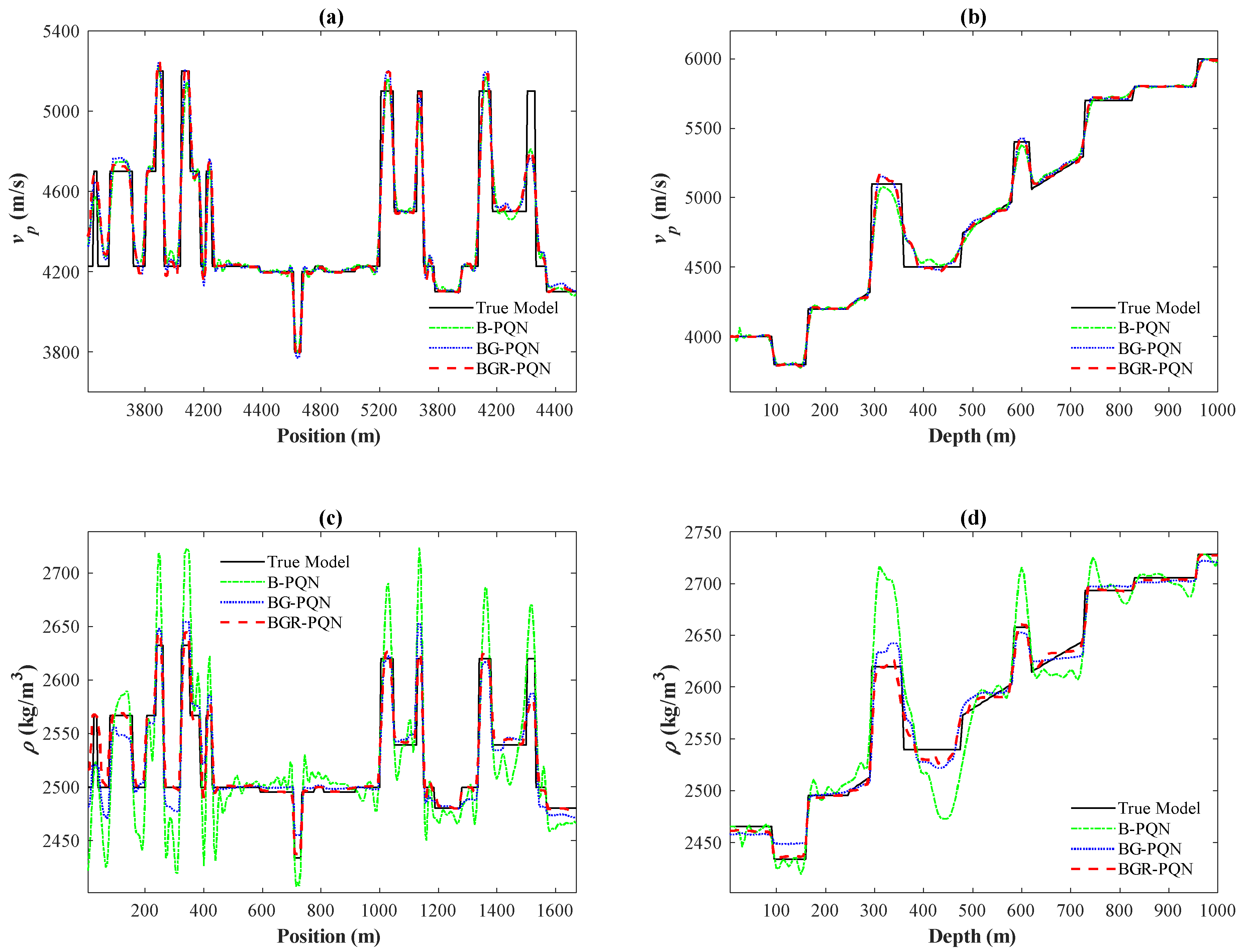
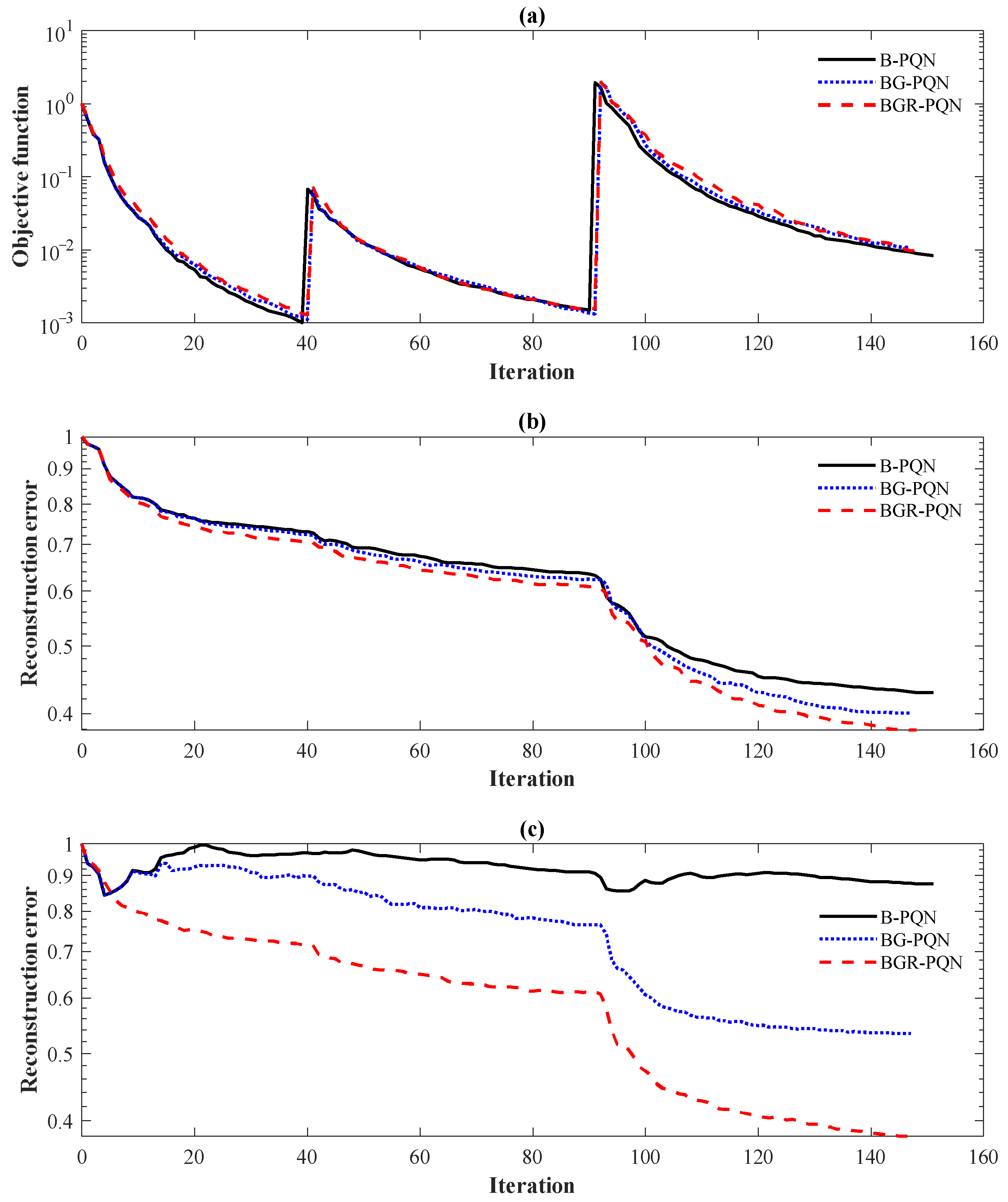
3.1.2. Multi-Constrained FWI Based on the PQN Algorithm

Selecting the bound constraint, gradient constraint, and rock-physical constraint as optional prior information, the following multi-constrained strategies are carried out in the multi-parameter FWI of the 1994BP model: (1) bound and gradient constrained based on the PQN algorithm (BG-PQN); and (2) bound, gradient and rock-physical constrained based on the PQN algorithm (BGR-PQN). For the 1994BP model, we set $s_{v_p}=6.18\times {10}^5$, $s_{\rho }=8.32\times {10}^4$ in Equation (4). Rock-physical relationship between the P-wave velocity and density satisfies $\ln \rho =0.25\ln v_p+5.7366$, $D_m$ in Equation (6) is set to 0.005.

Figure 7 shows the final multiscale inversion results, in which Figure 7a,b are P-wave velocity and density inversion results by the BG-PQN strategy, and Figure 7c,d show P-wave velocity and density inversion results of the BGR-PQN strategy. By comparing the recovered P-wave velocity models of the B-PQN strategy (Figure 3c) and the BG-PQN strategy (Figure 7a), it can be foun d that interfaces have poor continuity by adding a single bound constraint, especially when there are many artifacts in the area with large impedance difference at a depth of 200–500 m. After adding the gradient constraint, the multi-solution is better suppressed. The corresponding density inversion results show that the BG-PQN strategy improves the inversion greatly, the interfaces become clearer, and the model parameter is closer to the true model than that of the B-PQN strategy. Continuing to add rock-physical constraint, the artifacts in the recovered density model are further suppressed, and the parameter value is closer to the true model value.

In order to better analyze the impacts of rock-physical constraint on the inversion results, we draw a scatter plot of the P-wave velocity and the density as shown in Figure 8. It can be seen that after adding the boundary constraint and the gradient constraint, the inversion results are scattered around the true model data set in the scatter plot. After adding the rock-physical constraint, the P-wave velocity–density relationship of the model is closer to the real model.

A lateral section (section at z = 250 m indicated by the white dashed line AA′ in Figure 1a,b) and a vertical section (section at x = 800 m indicated by the white dashed line BB′ in Figure 1a,b) are selected for comparison of parameters. Figure 9 is the parameter sections of the B-PQN strategy, the BG-PQN strategy, and the BGR-PQN strategy in the 1994BP model. Figure 9a,b are inversion tangent diagrams of the P-wave velocity in sections AA′ and BB′, respectively. Compared with the multi-constrained strategy, the P-wave velocity inversion oscillates more obviously with the addition of a single boundary constraint, which deviates from the true model value. The BGR-PQN strategy has the best performance in P-wave velocity inversion accuracy, and the P-wave velocity curve obtained is more consistent with the real P-wave velocity. Compared with the single constrained strategy, the overall density inversion accuracy of the multi-constrained strategy has been significantly improved, especially in the region where the physical properties change drastically in the middle of the model. On the whole, the BGR-PQN strategy greatly improves the accuracy and stability of density inversion and performs well in the standard geological model test.

Figure 10a shows the convergence curves of the objective function in the experiments of the B-PQN strategy, the BG-PQN strategy, and the BGR-PQN strategy. The values of the objective function obtained by the above three strategies converge to a small value. Figure 10b shows the reconstruction error curves of the P-wave velocity. It can be seen that the error is the smallest under the BGR-PQN strategy, that is, the accuracy is the highest. Figure 10c is the reconstruction error curves of the density. The BGR-PQN strategy obtains a density model with a smaller error, and compared with the other two strategies, the advantages are obvious. In conclusion, the accuracy and stability of the inversion are significantly improved under the BGR-PQN strategy.

Table 2. Objective function, reconstruction error and calculation time of the 1994BP model under the B-PQN strategy, the BG-PQN strategy, and the BGR-PQN strategy.

Strategy	Objective Function	Reconstruction Error of P-Wave Velocity	Reconstruction Error of Density	Calculation Time
B-PQN	0.0083	0.4282	0.8760	3 h 55 min 10 s
BG-PQN	0.0109	0.4006	0.5337	5 h 3 min 26 s
BGR-PQN	0.0098	0.3788	0.3800	5 h 7 min 57 s

lists the objective function, reconstruction error of parameters, and calculation time of the 1994BP model under three different constrained strategies. It can be seen from the table that the accuracy of the P-wave velocity and the density has been greatly improved after adding the gradient constraint, but the value of the objective function is still large. Additionally, after continuing to add the rock-physical constraint, the accuracy of the density is further improved, and smaller objective function value is obtained in similar computation time.

In conclusion, the proposed PQN-based, multi-constrained, multi-parameter FWI framework is suitable for the seismic multi-parameter FWI problem, and can obtain a relatively stable and high-precision inversion model.

3.2. Overthrust Model

We use the overthrust model to test the inversion effect of the PQN-based multi-constrained, multi-parameter FWI algorithm under complex geological conditions. Firstly, we simplify the overthrust model. The original overthrust P-wave velocity model we used is shown in Figure 11a. We consider that the P-wave velocity and the density of the background medium satisfy the relation: $\ln \rho =0.25\ln v_p+5.7366$. The density model is shown in Figure 11b. The grid size of the model is 201 × 401, and the spatial interval ds = 10 m. When performing the multi-parameter FWI on the overthrust model, the initial model selects the model after Gaussian smoothing, as shown in Figure 11c,d. There is a total of 40 sources and 201 receivers located at surface level. The source is Ricker wavelet with peak frequency of 15 Hz. We also add Gaussian noise with S/N = 5 dB. For the multiscale inversion, three frequency bands 5 Hz, 10 Hz, and 15 Hz are used. The maximum number of iterations is set to 50 times in each frequency band.

The inversion experiments of unconstrained FWI (U-FWI) and multi-constrained FWI (C-FWI) are carried out. The inversion results without adding constraints are shown in Figure 12a,b. We added the boundary constraint in the first frequency band and the second frequency band, then added the boundary, gradient, and rock-physical constraints in the third frequency band. We set $L_{v_p}=6000$, $L_{\rho }=2614$, $U_{v_p}=2357$, and $U_{\rho }=2098$ in Equation (3); $s_{v_p}=6.30\times {10}^5$, $s_{\rho }=8.47\times {10}^4$ in Equation (4); and $a_n=0.2349$, $b_n=5.825$, and $D_m=0.01$ in Equation (6). The final inversion results of the overthrust model are shown in Figure 12c,d. Compared with unconstrained inversion, the multi-constrained inversion can show the stratigraphic interfaces more clearly and suppress the noise between strata, which has a more satisfactory inversion effect.

Figure 13 shows the records of the overthrust model, where (a) is the real record, (b) is the simulated record of the final inversion model, and (c) is the residual. It can be seen from Figure 13a that due to the addition of noise, some information in the record becomes blurred. The residual obtained by subtracting the real record from the simulated record of the final inversion model is essentially noise.

Figure 14 shows the convergence curves of the objective function in the above experiments, and (a), (b) and (c) are the curves under three scales, respectively. It can be seen that the curves of the two strategies are similar at the first two scales, but at the last scale, C-FWI is significantly lower than U-FWI, which is because the gradient constraint and rock-physics constraint are added at the last scale. At the same time, the value of the objective function does not decrease to a small value, which is due to the large amount of noise in the real record.

Table 3. Objective function, reconstruction error and calculation time of the overthrust model with the U-FWI and C-FWI strategies.

Strategy	Objective Function	Reconstruction Error of P-Wave Velocity	Reconstruction Error of Density	Calculation Time
U-FWI	1.1769	0.4399	0.4987	7 h 29 min 1 s
C-FWI	1.1763	0.4392	0.4380	7 h 35 min 8 s

lists objective function, the reconstruction error of parameters, and calculation time under different inversion strategies of the overthrust model. After adding compound constraints, the difference in calculation time is not significant, while the accuracy of P-wave velocity and density can be improved, especially the density.

In conclusion, our proposed PQN-based, multi-constrained, multi-parameter FWI framework is suitable for complex geological models and noise data.

4. Discussion

In the experiment of the 1994BP model, we compare the PQN algorithm with the SPG algorithm. The results show that the PQN algorithm has higher inversion accuracy and computational efficiency. Although we set the same maximum number of iteration in inversion, it must use line search to calculate the step length in each iteration. The update direction of the PQN algorithm is better than the SPG algorithm, so the number of forward modeling is less when the step length is calculated, which leads to the reduction of the overall calculation time. The PQN algorithm also combines the Hessian matrix information, which can improve the inversion. In the meantime, we also conduct experiment to compare the inversion strategies with different constraints (B-PQN, BG-PQN, and BGR-PQN), and the results show that with more information constraints, the inversion accuracy has been improved accordingly. The bound constraint makes the inversion parameter values not deviate from the regional geological conditions. In multi-parameter inversion, velocity and density have different properties. Velocity information not only affects amplitude but also affects phase, while density information only affects amplitude. Thus, density is often difficult to invert (Figure 3b,d). The rock-physical constraint can improve the density inversion results (Figure 7). Moreover, there are often some artifacts in the inversion results. The gradient constraint can be used to suppress noise and make the interface clear. Finally, the experiment of the overthrust model proves that the algorithm proposed in this paper is also applicable to complex models and noise data.

We also found that some constraints do not improve the low-frequency inversion results significantly, but produce a more obvious and positive effect on the high-frequency inversion. We think that the reason for this phenomenon may be that our constraints are of a smaller order of magnitude than the inversion results at lower frequencies. At higher frequencies, because the inversion results are relatively accurate, the constraints have a positive impact on the inversion results. Therefore, when carrying out the multiscale inversion, it is necessary to consider how to select the appropriate constraints and corresponding parameters at different scales. We recommend selecting simple constraints at low frequencies (such as boundary constraints) and selecting complex constraints at high frequencies (such as gradient and rock-physics constraints).

A question worthy of further discussion is the application of rock-physical constraints in FWI. Subsurface medium usually contains multiple types of rocks and fluids, and the rock-physical relationship is complex. In the experiments within this research, we verified that the proposed multi-parameter inversion framework is applicable to different models. However, for the application of rock-physical relationship constraints in geological models, we only carried out research in a relatively simple background medium. For more complex rock-physical relationships, it may be necessary to use mathematical statistics or deep learning for more reasonable classification and identification, helping us to maximize the rock-physical constraint in geophysical exploration. Furthermore, due to lithological variation and fluid content of geological media, it is important to take into account the attenuation of the medium [43,44]. Hence, moving from elastic FWI to viscoelastic FWI is also a good option to address the complexity of rock physics models.

5. Conclusions

This research constructs a multi-constrained, seismic multi-parameter FWI framework based on the PQN algorithm and uses the L-BFGS algorithm to obtain the Hessian matrix information.

The PQN algorithm is better than the SPG algorithm, which uses the Hessian matrix information and is more suitable for the multi-parameter FWI. Boundary constraints, gradient constraints, and rock-physical constraints are introduced in the multi-parameter FWI framework. These constraints make the inversion satisfy the different prior information conditions. The experiments of the 1994BP model and the overthrust model show that the framework can effectively improve the inversion accuracy and is applicable to noise data.

The proposed multi-constrained FWI framework can be compatible with other prior information constraints. Representing more prior geological information as constraints in mathematical form, including the dip of strata, the orientation of regional structures, etc., will further improve the effect of inversion. This is the content of our follow-up work.

References

1. Tarantola, A. Inversion of seismic reflection data in the acoustic approximation. Geophysics 1984, 49, 1259–1266. [Google Scholar] [CrossRef]
2. Mora, P.; Wu, Z. Elastic versus acoustic inversion for marine surveys. Geophys. J. Int. 2018, 14, 596–622. [Google Scholar] [CrossRef]
3. Takougang, E.M.T.; Ali, M.Y.; Bouzidi, Y.; Bouchaala, F.; Sultan, A.A.; Mohamed, A.I. Characterization of a carbonate reservoir using elastic full-waveform inversion of vertical seismic profile data. Geophys. Prospect. 2020, 68, 1944–1957. [Google Scholar] [CrossRef]
4. Shi, Y.M.; Yao, F.C.; Sun, H.S.; Qi, L. Density inversion and porosity estimation. Chin. J. Geophys-Chin. 2010, 53, 197–204. [Google Scholar]
5. Jeong, W.; Lee, H.Y.; Min, D.J. Full waveform inversion strategy for density in the frequency domain. Geophys. J. Int. 2012, 188, 1221–1242. [Google Scholar] [CrossRef]
6. Yang, J.Z.; Liu, Y.Z.; Dong, L.G. A multi-parameter inversion strategy for acoustic media with variable density. Chin. J. Geophys. 2014, 57, 628–643. [Google Scholar]
7. Zhang, Z.D.; Alkhalifah, T.; Naeini, E.Z.; Sun, B. Multiparameter elastic full waveform inversion with facies-based constraints. Geophys. J. Int. 2018, 213, 2112–2127. [Google Scholar] [CrossRef]
8. Sun, M.; Jin, S. Multiparameter elastic full waveform inversion of ocean bottom seismic four-component data based on a modified acoustic-elastic coupled equation. Remote Sens. 2020, 12, 2816. [Google Scholar] [CrossRef]
9. Virieux, J.; Operto, S. An Overview of Full-Waveform Inversion in Exploration Geophysics. Geophysics 2009, 74, WCC127–WCC152. [Google Scholar] [CrossRef]
10. Operto, S.; Gholami, Y.; Prieux, V.; Ribodetti, A.; Brossier, R.; Metivier, L.; Virieux, J. A guided tour of multiparameter full-waveform inversion with multicomponent data: From theory to practice. Lead. Edge 2013, 32, 1005–1176. [Google Scholar] [CrossRef]
11. Song, C.; Alkhalifah, T. An efficient wavefield inversion for transversely isotropic media with a vertical axis of symmetry. Geophysics 2020, 85, R195–R206. [Google Scholar] [CrossRef]
12. Vogel, C.R. Computational Methods for Inverse Problems; SIAM Press: Philadelphia, PA, USA, 2002. [Google Scholar]
13. Asnaashari, A.; Brossier, R.; Garambois, S.; Audebert, F.; Thore, P.; Virieux, J. Regularized seismic full waveform inversion with prior model information. Geophysics 2013, 78, R25–R36. [Google Scholar] [CrossRef]
14. Gao, K.; Huang, L. Acoustic- and elastic-waveform inversion with total generalized p-variation regularization. Geophys. J. Int. 2019, 218, 933–957. [Google Scholar] [CrossRef]
15. Feng, D.S.; Wang, X.; Wang, X.Y. New Dynamic Stochastic Source Encoding Combined with a Minmax-Concave Total Variation Regularization Strategy for Full Waveform Inversion. IEEE Tran. Geosci. Remote Sens. 2020, 58, 7753–7771. [Google Scholar] [CrossRef]
16. Aghamiry, H.S.; Holami, A.; Operto, S. Compound Regularization of Full-Waveform Inversion for Imaging Piecewise Media. IEEE Trans. Geosci. Remote Sens. 2020, 58, 1192–1204. [Google Scholar] [CrossRef]
17. Du, Z.; Liu, D.; Wu, G.; Cai, J.; Yu, X.; Hu, G. A high-order total-variation regularisation method for full-waveform inversion. J. Geophys. Eng. 2021, 18, 241–252. [Google Scholar] [CrossRef]
18. Qu, S.; Verschuur, E.; Chen, Y. Full-waveform inversion and joint migration inversion with an automatic directional total variation constraint. Geophysics 2019, 84, R175–R183. [Google Scholar] [CrossRef]
19. Peters, B.; Herrmann, F.J. Constraints versus penalties for edge-preserving full-waveform inversion. Lead. Edge 2017, 36, 94–100. [Google Scholar] [CrossRef]
20. Lin, Y.; Huang, L. Acoustic- and elastic-waveform inversion using a modified total-variation regularization scheme. Geophys. J. Int. 2015, 200, 489–502. [Google Scholar] [CrossRef]
21. Smithyman, B.R.; Peters, B.; Herrmann, F.J. Constrained waveform inversion of colocated VSP and surface seismic data. In Proceedings of the 77th EAGE Conference and Exhibition, Madrid, Spain, 1–4 June 2015. [Google Scholar]
22. Birgin, E.G.; Martínez, J.M.; Raydan, M. Nonmonotone spectral projected gradient methods on convex sets. SIAM J. Optim. 2000, 10, 1196–1211. [Google Scholar] [CrossRef]
23. Xu, H.K. Averaged Mappings and the Gradient-Projection Algorithm. J. Optim. Theory Appl. 2011, 150, 360–378. [Google Scholar] [CrossRef]
24. Yao, Y.; Liou, Y.C.; Wen, C.F. Variant Gradient Projection Methods for the Minimization Problems. Abstr. Appl. Anal. 2012, 2012, 792078. [Google Scholar] [CrossRef]
25. Gomes-Ruggiero, M.A.; Martinez, J.M.; Santos, S.A. Spectral projected gradient method with inexact restoration for minimization with nonconvex constraints. SIAM J. Sci. Comput. 2009, 31, 1628–1652. [Google Scholar] [CrossRef]
26. Peters, B.; Smithyman, B.R.; Herrmann, F.J. Projection methods and applications for seismic nonlinear inverse problems with multiple constraints. Geophysics 2019, 84, R251–R269. [Google Scholar] [CrossRef]
27. Jiang, W. 3-D joint inversion of seismic waveform and airborne gravity gradiometry data. Geophys. J. Int. 2020, 223, 746–764. [Google Scholar] [CrossRef]
28. Rao, J.; Yang, J.; Ratasseppc, M.; Fan, Z. Multi-parameter reconstruction of velocity and density using ultrasonic tomography based on full waveform inversion. Ultrasonics 2020, 101, 106004. [Google Scholar] [CrossRef] [PubMed]
29. Xu, K.; McMechan, G.A. 2D frequency-domain elastic full-waveform inversion using time-domain modeling and a multistep-length gradient approach. Geophysics 2014, 79, R41–R53. [Google Scholar] [CrossRef]
30. Alkhalifah, T. Scattering-angle based filtering of the waveform inversion gradients. Geophys. J. Int. 2014, 200, 363–373. [Google Scholar] [CrossRef]
31. Cheng, J.; Alkhalifah, T.; Wu, Z.; Zou, P.; Wang, C. Simulating propagation of decoupled elastic waves using low-rank approximate mixed-domain integral operators for anisotropic media. Geophysics 2016, 81, T63–T77. [Google Scholar] [CrossRef]
32. Wang, T.F.; Cheng, J.B. Elastic full waveform inversion based on mode decomposition: The approach and mechanism. Geophys. J. Int. 2017, 209, 606–622. [Google Scholar] [CrossRef]
33. Schmidt, M.; Berg, E.; Friedlander, M.P.; Murphy, K. Optimizing Costly Functions with Simple Constraints: A Limited-Memory Projected Quasi-Newton Algorithm. Artif. Intell. Stat. 2009, 5, 456–463. [Google Scholar]
34. Kim, D.; Sra, S.; Dhillon, I.S. Tackling box-constrained optimization via a new projected quasi-newton approach. SIAM J. Sci. Comput. 2010, 32, 3548–3563. [Google Scholar] [CrossRef]
35. van den Berg, E. A hybrid quasi-Newton projected-gradient method with application to Lasso and basis-pursuit denoising. Math. Program. Comput. 2020, 12, 1–38. [Google Scholar] [CrossRef]
36. Rothermel, D.; Schuster, T. Solving an inverse heat convection problem with an implicit forward operator by using a projected quasi-Newton method. Inverse Probl. 2021, 37, 045014. [Google Scholar] [CrossRef]
37. Liu, D.C.; Nocedal, J. On the limited memory BFGS method for large scale optimization. Math. Program. 1989, 45, 503–528. [Google Scholar] [CrossRef]
38. Byrd, R.H.; Nocedal, J.; Schnabel, R.B. Representations of quasi-newton matrices and their use in limited memory methods. Math. Program. 1994, 63, 129–156. [Google Scholar] [CrossRef]
39. Sirgue, L.; Pratt, R.G. Efficient waveform inversion and imaging: A strategy for selecting temporal frequencies. Geophysics 2004, 69, 231–248. [Google Scholar] [CrossRef]
40. Boonyasiriwat, C.; Valasek, P.; Routh, P.S.; Cao, W.; Schuster, G.T.; Macy, B. An efficient multiscale method for time-domain waveform tomography. Geophysics 2009, 74, WCC59–WCC68. [Google Scholar] [CrossRef]
41. Gardner, G.H.F.; Gardner, L.W.; Gregory, A.R. Formation velocity and density—The diagnostic basics for stratigraphic traps. Geophysics 1974, 39, 770–780. [Google Scholar] [CrossRef]
42. He, B.S.; Yang, H.; Wang, S.L. Alternating direction method with self-adaptive penalty parameters for monotone variational inequalities. J. Optim. Theory Appl. 2000, 106, 337–356. [Google Scholar] [CrossRef]
43. Yang, P.; Brossier, R.; Métivier, L.; Virieux, J. A review on the systematic formulation of 3-D multiparameter full waveform inversion in viscoelastic medium. Geophys. J. Int. 2016, 207, 129–149. [Google Scholar] [CrossRef]
44. Bouchaala, F.; Ali, M.Y.; Matsushima, J. Compressional and shear wave attenuations from walkway VSP and sonic data in an offshore Abu Dhabi oilfield. Géoscience 2021, 353, 337–354. [Google Scholar] [CrossRef]
45. Plessix, R.E. A review of the adjoint-state method for computing the gradient of a functional with geophysical applications. Geophys. J. Int. 2006, 167, 495–503. [Google Scholar] [CrossRef]
Figure 1. The P-wave velocity model (a), the density model (b), the P-wave initial velocity model (c), and the initial density model (d) of the 1994BP model.
Remotesensing 15 02416 g001
Figure 2. One of the records for inversion of the 1994BP model.
Remotesensing 15 02416 g002
Figure 3. The recovered P-wave velocity model (a) and the recovered density model (b) by the B-SPG strategy of the 1994BP model, and the recovered P-wave velocity model (c) and the recovered density model (d) by the B-PQN strategy of the 1994BP model.
Remotesensing 15 02416 g003
Figure 4. The difference between the true model and the recovered model. (a,b) are the difference of P-wave velocity and density by the B-SPG strategy, respectively; (c,d) are the difference of P-wave velocity and density by the B-PQN strategy, respectively.
Remotesensing 15 02416 g004
Figure 5. Parameter sections in the 1994BP model. (a) Section of P-wave velocity at z = 250 m, (b) Section of P-wave velocity at x = 800 m, (c) Section of density at z = 250 m, and (d) Section of density at x = 800 m. Black solid lines represent the true model value, blue dotted lines represent the inversion results of the B-SPG strategy, and red dashed lines represent the inversion results of the B-PQN strategy.
Remotesensing 15 02416 g005
Figure 6. Objective function curves (a) and reconstruction error curves (b) of the 1994BP model under the B-SPG strategy and the B-PQN strategy. Black lines represent the inversion results of the B-SPG strategy, and red lines represent the inversion results of the B-PQN strategy. The solid lines in (b) are reconstruction error curves of P-wave velocity, and the dashed lines in (b) represent reconstruction error curves of density.
Remotesensing 15 02416 g006
Figure 7. Recovered P-wave velocity model by the BG-PQN strategy: (a) recovered density model by the BG-PQN strategy; (b) recovered P-wave velocity model by the BGR-PQN strategy; and (c) recovered density model by the BGR-PQN strategy (d).
Remotesensing 15 02416 g007
Figure 8. P-wave velocity-density scatter plot of the 1994BP model. White circles represent the true model, blue circles represent the inversion results of the BG-PQN strategy, and red circles represent the inversion results of the BGR-PQN strategy. The green line is the fitting line of the true model.
Remotesensing 15 02416 g008
Figure 9. Parameter sections of the B-PQN strategy, the BG-PQN strategy, and the BGR-PQN strategy in the 1994BP model: (a) section of P-wave velocity at z = 250 m; (b) section of P-wave velocity at x = 800 m; (c) section of density at z = 250 m; and (d) section of density at x = 800 m. Black solid lines represent the true model, green dot-dashed lines are the inversion results of the B-PQN strategy, blue dotted lines show the BG-PQN strategy inversion results, and red dashed lines represent the results of the BGR-PQN strategy.
Remotesensing 15 02416 g009
Figure 10. Objective function curves: (a) reconstruction error curves of the P-wave velocity; and (b) reconstruction error curves of the density (c) in the 1994BP model. Black solid lines represent the inversion results of the B-PQN strategy, blue dotted lines represent the inversion results of the BG-PQN strategy, and red lines represent the inversion results of the BGR-PQN strategy.
Remotesensing 15 02416 g010
Figure 11. True P-wave velocity model: (a) true density model; (b) initial P-wave velocity model; and (c) initial density model (d) of the overthrust model.
Remotesensing 15 02416 g011
Figure 12. Inversion results of the overthrust model: (a) the recovered P-wave velocity model; the recovered density model (b) by the U-FWI strategy; the recovered P-wave velocity model (c); and the recovered density model (d) by the C-FWI strategy.
Remotesensing 15 02416 g012
Figure 13. The records for the overthrust model: (a) is the real record; (b) is the simulated record of the final inversion model; and (c) is the residual.
Remotesensing 15 02416 g013
Figure 14. Objective function curves of the overthrust model under the U-FWI strategy and the C-FWI strategy: (ac) are the curves in three scales, respectively. Black lines represent the inversion results of the U-FWI strategy, and red lines represent the inversion results of the C-FWI strategy.
Remotesensing 15 02416 g014