
Dual-Level Contextual Attention Generative Adversarial Network for Reconstructing SAR Wind Speeds in Tropical Cyclones

 , , , ,
  , , and
Abstract
1. Introduction
- We propose a GAN-based deep learning model for directly enhancing the quality of SAR wind speeds and reconstructing the structure of TCs. The results are based on SAR observations and are close to reality, and thus can be used for TC intensity estimation, TC structure analysis, and forecast accuracy improvement.
- The proposed model performs better than state-of-the-art models, especially for a large range of low-quality data and in high wind speed reconstruction. We also conduct ablation experiments to verify the components’ effectiveness in the proposed model.
- The model is validated on ECMWF and SMAP, and the reconstructed results can be obtained in a few seconds using a single GPU. Compared to ECMWF, the reconstructed results achieve a relative reduction of 50% in the root mean square error (RMSE).
2. Method
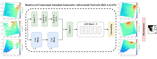
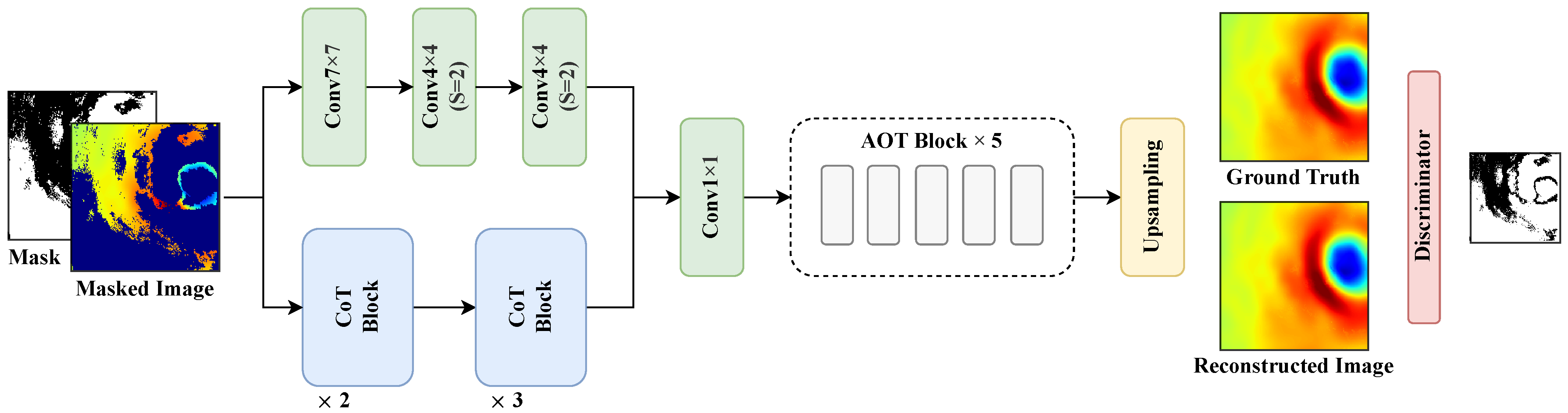
2.1. Architecture
2.2. Encoder Based on Dual-Level Learning
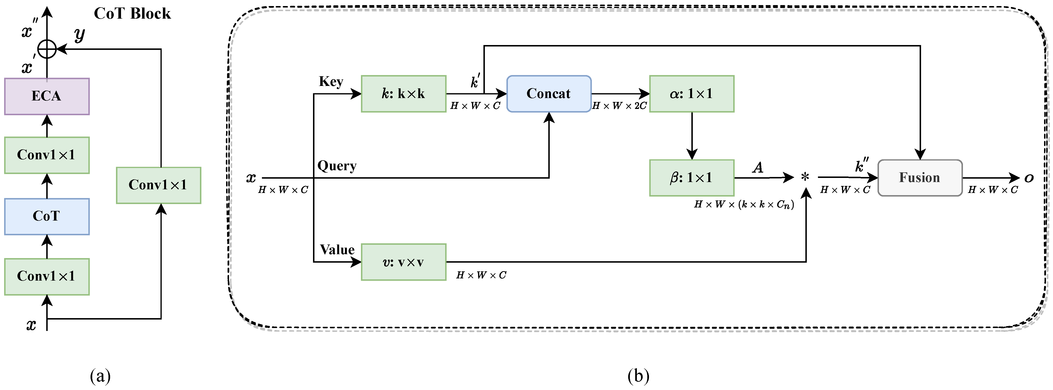
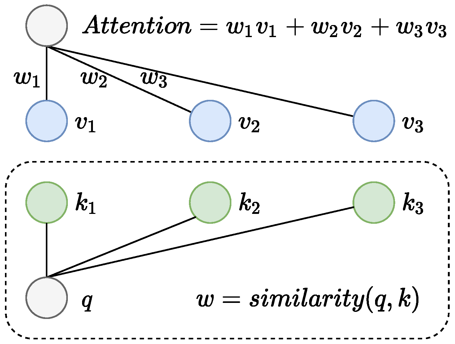
2.2.1. CoT Block
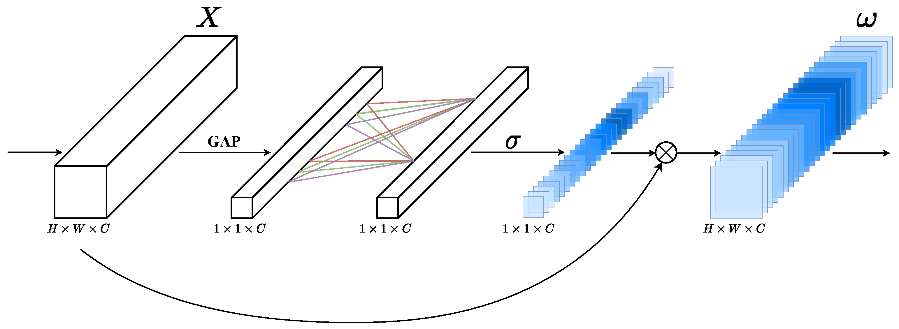
2.2.2. ECA Module
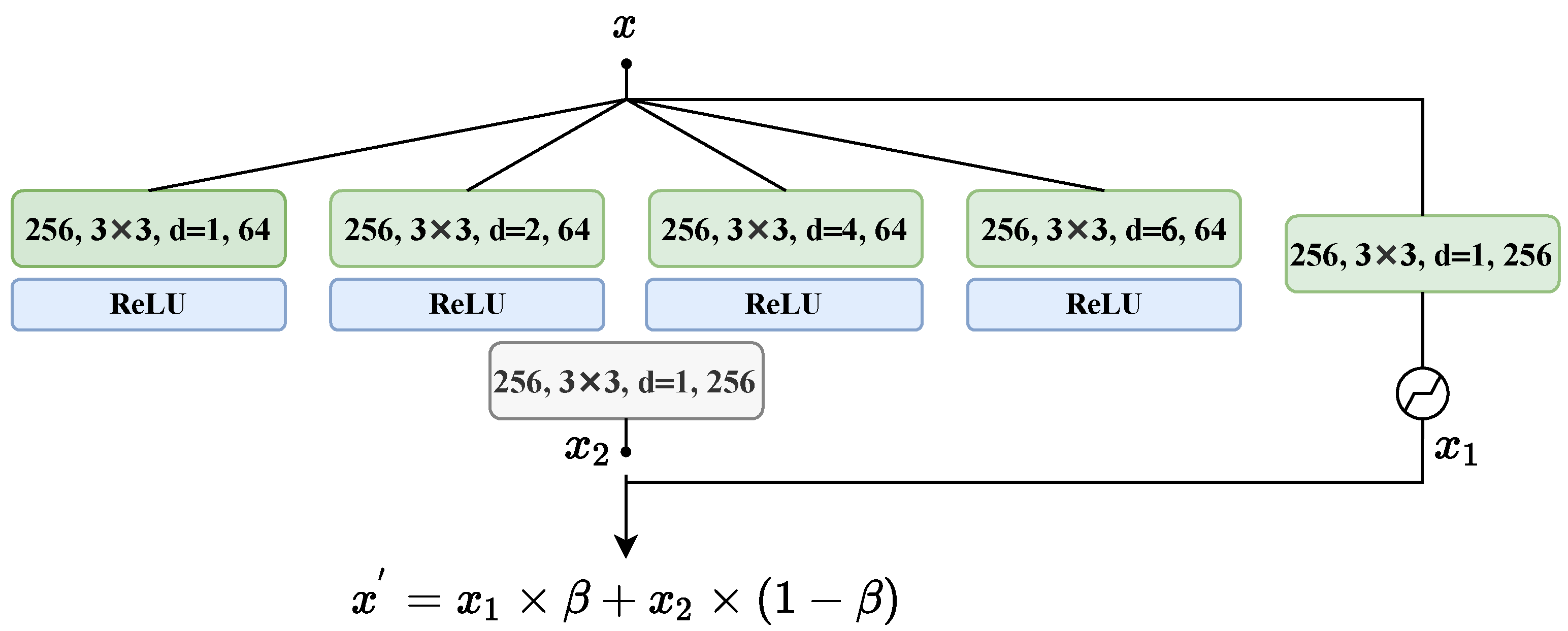
2.3. AOT Neck
2.4. Loss
2.4.1. SM-PatchGAN
2.4.2. Joint Loss
3. Experiments
3.1. Data
3.2. Experiment Configuration and Implementation Details
3.3. Evaluation Metric
3.4. Experimental Results
- PConv [51] proposes to replace vanilla convolution with partial convolution to reduce the color discrepancy in the missing area.
- GatedConv [50] is a two-stage network: the first stage outputs coarse results and the second stage is for finer ones. This structure can progressively increase the smoothness of the reconstructed image. The work also proposes an SN-PatchGAN for training.
- AOT-GAN [30] aggregates the feature maps of different receptive fields to improve the reconstruction effect of high-resolution images.
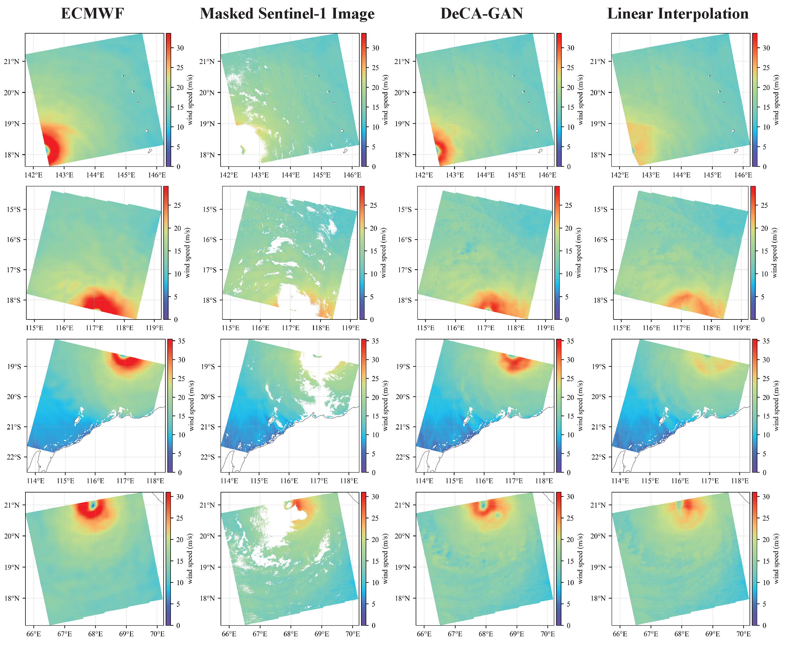
3.4.1. Comparison of DeCA-GAN to Baselines
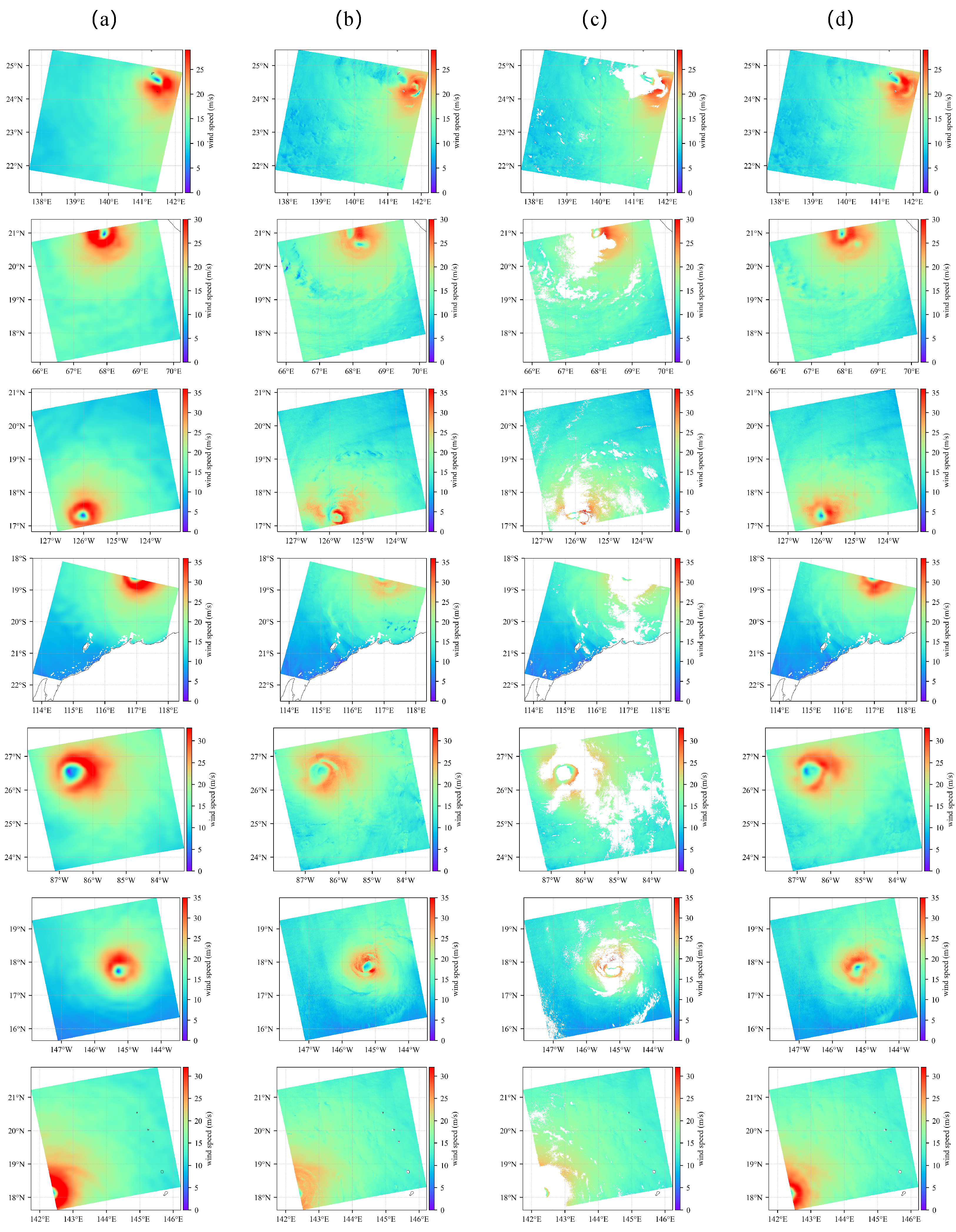
3.4.2. Reconstruction on Sentinel1-A/B
3.5. Ablation Studies
3.5.1. Dual-Level Encoder
3.5.2. Number of AOT Blocks
3.5.3. Benefits of Adversarial Loss
3.6. Visualization of DeCA-GAN Internal Feature Maps
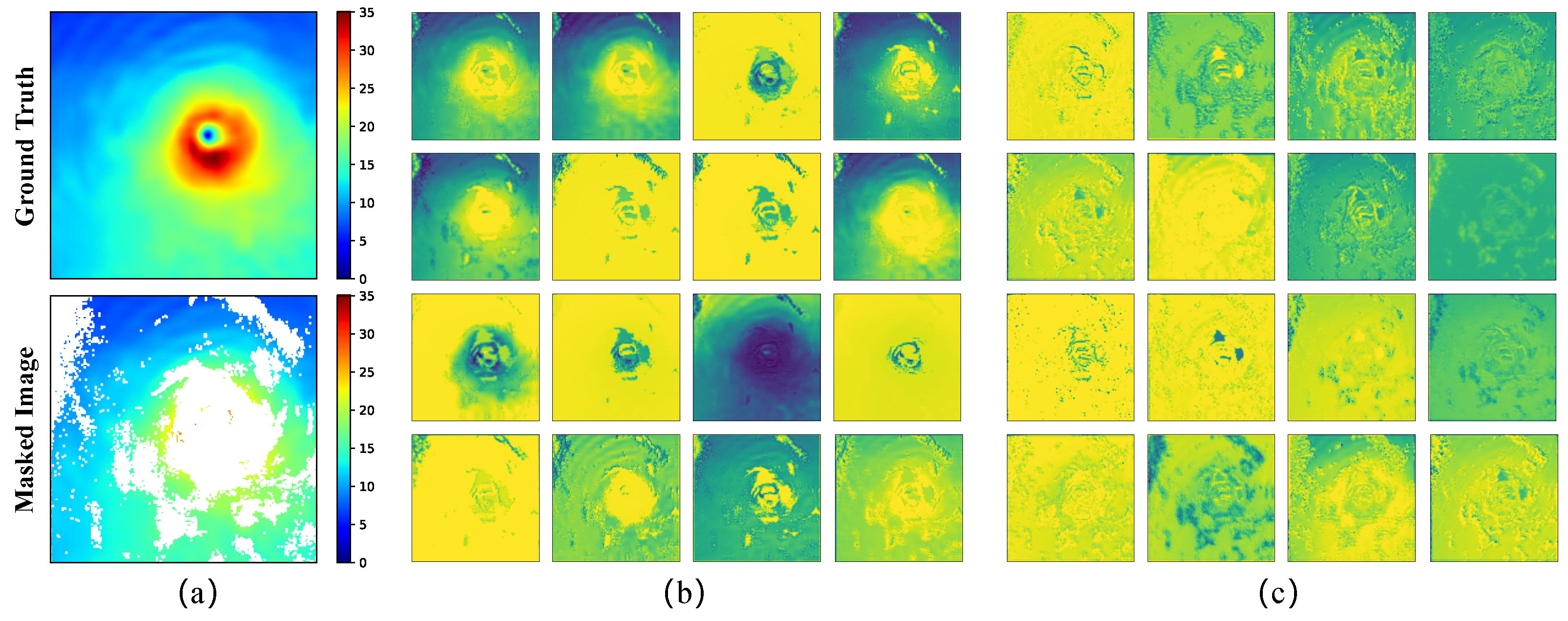
3.6.1. Features Learned by the Dual-Level Encoder
3.6.2. Feature Integration by AOT Blocks
4. Discussion
- We collected 270 ECMWF data and divided them into training and validation sets. However, for DL algorithms, this amount of data is still relatively small. In addition, ECMWF and SAR wind speeds belong to different distributions, resulting in degraded performance when reconstructing SAR observations directly. We will continue to expand the amount of data or introduce some techniques to obtain data closer to the SAR distribution.
- The DeCA-GAN was trained based on ECMWF wind speed data as labels. ECMWF is a very commonly used dataset in the wind speed retrieval of remote sensing satellites. However, some studies have shown that ECMWF underestimates high wind speeds [58,59], which may lead to some bias in the features learned by the proposed model. This point is also confirmed by the comparison with SMAP, which indicates that our model tends to underestimate wind speeds in high wind speed ranges. The next step is to train the model using the Hurricane Weather Research and Forecasting wind speed.
5. Conclusions
Author Contributions
Funding
Data Availability Statement
Conflicts of Interest
References
- Gray, W.M. Tropical Cyclone Genesis. Ph.D. Thesis, Colorado State University, Fort Collins, CO, USA, 1975. [Google Scholar]
- Emanuel, K. Tropical cyclones. Annu. Rev. Earth Planet. Sci. 2003, 31, 75–104. [Google Scholar] [CrossRef]
- Peduzzi, P.; Chatenoux, B.; Dao, H.; De Bono, A.; Herold, C.; Kossin, J.; Mouton, F.; Nordbeck, O. Global trends in tropical cyclone risk. Nat. Clim. Change 2012, 2, 289–294. [Google Scholar] [CrossRef]
- Katsaros, K.B.; Vachon, P.W.; Black, P.G.; Dodge, P.P.; Uhlhorn, E.W. Wind fields from SAR: Could they improve our understanding of storm dynamics? Johns Hopkins APL Tech. Digest 2000, 21, 86–93. [Google Scholar] [CrossRef]
- Tiampo, K.F.; Huang, L.; Simmons, C.; Woods, C.; Glasscoe, M.T. Detection of Flood Extent Using Sentinel-1A/B Synthetic Aperture Radar: An Application for Hurricane Harvey, Houston, TX. Remote Sens. 2022, 14, 2261. [Google Scholar] [CrossRef]
- Soria-Ruiz, J.; Fernández-Ordoñez, Y.M.; Chapman, B. Radarsat-2 and Sentinel-1 Sar to Detect and Monitoring Flooding Areas in Tabasco, Mexico. In Proceedings of the 2021 IEEE International Geoscience and Remote Sensing Symposium IGARSS, Brussels, Belgium, 11–16 July 2021; pp. 1323–1326. [Google Scholar] [CrossRef]
- Sentinel-1 Ocean Wind Fields (OWI) Algorithm Definition. Available online: https://sentinel.esa.int/documents/247904/4766122/DI-MPC-IPF-OWI_2_1_OWIAlgorithmDefinition.pdf/ (accessed on 3 April 2023).
- Hwang, P.A.; Zhang, B.; Perrie, W. Depolarized radar return for breaking wave measurement and hurricane wind retrieval. Geophys. Res. Lett. 2010, 37. [Google Scholar] [CrossRef]
- Vachon, P.W.; Wolfe, J. C-band cross-polarization wind speed retrieval. IEEE Geosci. Remote Sens. Lett. 2010, 8, 456–459. [Google Scholar] [CrossRef]
- de Kloe, J.; Stoffelen, A.; Verhoef, A. Improved use of scatterometer measurements by using stress-equivalent reference winds. IEEE J. Sel. Top. Appl. Earth Obs. Remote Sens. 2017, 10, 2340–2347. [Google Scholar] [CrossRef]
- Shen, H.; Perrie, W.; He, Y.; Liu, G. Wind speed retrieval from VH dual-polarization RADARSAT-2 SAR images. IEEE Trans. Geosci. Remote Sens. 2013, 52, 5820–5826. [Google Scholar] [CrossRef]
- Zhang, B.; Perrie, W. Cross-polarized synthetic aperture radar: A new potential measurement technique for hurricanes. Bull. Am. Meteorol. Soc. 2012, 93, 531–541. [Google Scholar] [CrossRef]
- Zhang, G.; Li, X.; Perrie, W.; Hwang, P.A.; Zhang, B.; Yang, X. A hurricane wind speed retrieval model for C-band RADARSAT-2 cross-polarization ScanSAR images. IEEE Trans. Geosci. Remote Sens. 2017, 55, 4766–4774. [Google Scholar] [CrossRef]
- Zhang, G.; Perrie, W. Symmetric double-eye structure in hurricane bertha (2008) imaged by SAR. Remote Sens. 2018, 10, 1292. [Google Scholar] [CrossRef]
- Zhang, G.; Perrie, W.; Zhang, B.; Yang, J.; He, Y. Monitoring of tropical cyclone structures in ten years of RADARSAT-2 SAR images. Remote Sens. Environ. 2020, 236, 111449. [Google Scholar] [CrossRef]
- Zhang, B.; Zhu, Z.; Perrie, W.; Tang, J.; Zhang, J.A. Estimating tropical cyclone wind structure and intensity from spaceborne radiometer and synthetic aperture radar. IEEE J. Sel. Top. Appl. Earth Obs. Remote Sens. 2021, 14, 4043–4050. [Google Scholar] [CrossRef]
- Portabella, M.; Stoffelen, A.; Johannessen, J.A. Toward an optimal inversion method for synthetic aperture radar wind retrieval. J. Geophys. Res. Oceans 2002, 107, 1-1-1-13. [Google Scholar] [CrossRef]
- Ye, X.; Lin, M.; Zheng, Q.; Yuan, X.; Liang, C.; Zhang, B.; Zhang, J. A typhoon wind-field retrieval method for the dual-polarization SAR imagery. IEEE Geosci. Remote Sens. Lett. 2019, 16, 1511–1515. [Google Scholar] [CrossRef]
- Boussioux, L.; Zeng, C.; Guénais, T.; Bertsimas, D. Hurricane forecasting: A novel multimodal machine learning framework. Weather Forecast. 2022, 37, 817–831. [Google Scholar] [CrossRef]
- Carmo, A.R.; Longépé, N.; Mouche, A.; Amorosi, D.; Cremer, N. Deep Learning Approach for Tropical Cyclones Classification Based on C-Band Sentinel-1 SAR Images. In Proceedings of the 2021 IEEE International Geoscience and Remote Sensing Symposium IGARSS, Brussels, Belgium, 11–16 July 2021; pp. 3010–3013. [Google Scholar] [CrossRef]
- Li, X.M.; Qin, T.; Wu, K. Retrieval of sea surface wind speed from spaceborne SAR over the Arctic marginal ice zone with a neural network. Remote Sens. 2020, 12, 3291. [Google Scholar] [CrossRef]
- Funde, K.; Joshi, J.; Damani, J.; Jyothula, V.R.; Pawar, R. Tropical Cyclone Intensity Classification Using Convolutional Neural Networks On Satellite Imagery. In Proceedings of the 2022 International Conference on Industry 4.0 Technology (I4Tech), Pune, India, 23–24 September 2022; pp. 1–5. [Google Scholar] [CrossRef]
- Yu, P.; Xu, W.; Zhong, X.; Johannessen, J.A.; Yan, X.H.; Geng, X.; He, Y.; Lu, W. A Neural Network Method for Retrieving Sea Surface Wind Speed for C-Band SAR. Remote Sens. 2022, 14, 2269. [Google Scholar] [CrossRef]
- Mu, S.; Li, X.; Wang, H. The Fusion of Physical, Textural and Morphological Information in SAR Imagery for Hurricane Wind Speed Retrieval Based on Deep Learning. IEEE Trans. Geosci. Remote Sens. 2022, 60, 1–13. [Google Scholar] [CrossRef]
- Nezhad, M.M.; Heydari, A.; Pirshayan, E.; Groppi, D.; Garcia, D.A. A novel forecasting model for wind speed assessment using sentinel family satellites images and machine learning method. Renew. Energy 2021, 179, 2198–2211. [Google Scholar] [CrossRef]
- Goodfellow, I.J.; Pouget-Abadie, J.; Mirza, M.; Xu, B.; Warde-Farley, D.; Ozair, S.; Courville, A.C.; Bengio, Y. Generative Adversarial Nets. In Proceedings of the Advances in Neural Information Processing Systems 27: Annual Conference on Neural Information Processing Systems 2014, Montreal, QC, Canada, 8–13 December 2014; pp. 2672–2680. [Google Scholar]
- Yu, F.; Koltun, V. Multi-Scale Context Aggregation by Dilated Convolutions. In Proceedings of the 4th International Conference on Learning Representations, San Juan, Puerto Rico, 2–4 May 2016. [Google Scholar]
- Vaswani, A.; Shazeer, N.; Parmar, N.; Uszkoreit, J.; Jones, L.; Gomez, A.N.; Kaiser, L.; Polosukhin, I. Attention is All you Need. In Proceedings of the Advances in Neural Information Processing Systems 30: Annual Conference on Neural Information Processing Systems 2017, Long Beach, CA, USA, 4–9 December 2017; pp. 5998–6008. [Google Scholar]
- Li, Y.; Yao, T.; Pan, Y.; Mei, T. Contextual transformer networks for visual recognition. IEEE Trans. Pattern Anal. Mach. Intell. 2022, 45, 1489–1500. [Google Scholar] [CrossRef]
- Zeng, Y.; Fu, J.; Chao, H.; Guo, B. Aggregated contextual transformations for high-resolution image inpainting. IEEE Trans. Visual Comput. Graphics 2022. [Google Scholar] [CrossRef]
- Wang, Q.; Wu, B.; Zhu, P.; Li, P.; Zuo, W.; Hu, Q. ECA-Net: Efficient Channel Attention for Deep Convolutional Neural Networks. In Proceedings of the 2020 IEEE/CVF Conference on Computer Vision and Pattern Recognition, CVPR 2020, Seattle, WA, USA, 13–19 June 2020; pp. 11531–11539. [Google Scholar] [CrossRef]
- Wang, P.; Chen, P.; Yuan, Y.; Liu, D.; Huang, Z.; Hou, X.; Cottrell, G. Understanding convolution for semantic segmentation. In Proceedings of the 2018 IEEE Winter Conference on Applications of Computer Vision (WACV), Lake Tahoe, NV, USA, 12–15 March 2018; pp. 1451–1460. [Google Scholar] [CrossRef]
- Mottaghi, R.; Chen, X.; Liu, X.; Cho, N.; Lee, S.; Fidler, S.; Urtasun, R.; Yuille, A.L. The Role of Context for Object Detection and Semantic Segmentation in the Wild. In Proceedings of the 2014 IEEE Conference on Computer Vision and Pattern Recognition, CVPR 2014, Columbus, OH, USA, 23–28 June 2014; pp. 891–898. [Google Scholar] [CrossRef]
- Rabinovich, A.; Vedaldi, A.; Galleguillos, C.; Wiewiora, E.; Belongie, S.J. Objects in Context. In Proceedings of the IEEE 11th International Conference on Computer Vision, ICCV 2007, Rio de Janeiro, Brazil, 14–20 October 2007; pp. 1–8. [Google Scholar] [CrossRef]
- Zeng, X.; Ouyang, W.; Wang, X. Multi-stage Contextual Deep Learning for Pedestrian Detection. In Proceedings of the IEEE International Conference on Computer Vision, ICCV 2013, Sydney, Australia, 1–8 December 2013; pp. 121–128. [Google Scholar] [CrossRef]
- Tan, Z.; Wang, M.; Xie, J.; Chen, Y.; Shi, X. Deep Semantic Role Labeling With Self-Attention. In Proceedings of the AAAI (Thirty-Second AAAI Conference on Artificial Intelligence), New Orleans, LA, USA, 2–7 February 2018; pp. 4929–4936. [Google Scholar]
- Verga, P.; Strubell, E.; McCallum, A. Simultaneously Self-Attending to All Mentions for Full-Abstract Biological Relation Extraction. In Proceedings of the NAACL-HLT (North American Chapter of the Association for Computational Linguistics: Human Language Technologies), New Orleans, LA, USA, 1–6 June 2018; pp. 872–884. [Google Scholar] [CrossRef]
- Devlin, J.; Chang, M.W.; Lee, K.; Toutanova, K. BERT: Pre-training of Deep Bidirectional Transformers for Language Understanding. In Proceedings of the NAACL-HLT 2019, Minneapolis, MN, USA, 2–7 June 2019; pp. 4171–4186. [Google Scholar] [CrossRef]
- Dosovitskiy, A.; Beyer, L.; Kolesnikov, A.; Weissenborn, D.; Zhai, X.; Unterthiner, T.; Dehghani, M.; Minderer, M.; Heigold, G.; Gelly, S.; et al. An image is worth 16x16 words: Transformers for image recognition at scale. arXiv 2020, arXiv:2010.11929. [Google Scholar]
- Carion, N.; Massa, F.; Synnaeve, G.; Usunier, N.; Kirillov, A.; Zagoruyko, S. End-to-end object detection with transformers. In Computer Vision–ECCV 2020: Proceedings of the 16th European Conference, Glasgow, UK, 23–28 August 2020; Springer: Berlin/Heidelberg, Germany, 2020; pp. 213–229. [Google Scholar]
- Liu, Z.; Lin, Y.; Cao, Y.; Hu, H.; Wei, Y.; Zhang, Z.; Lin, S.; Guo, B. Swin transformer: Hierarchical vision transformer using shifted windows. In Proceedings of the IEEE/CVF International Conference on Computer Vision, Montreal, BC, Canada, 11–17 October 2021; pp. 10012–10022. [Google Scholar] [CrossRef]
- Ramachandran, P.; Parmar, N.; Vaswani, A.; Bello, I.; Levskaya, A.; Shlens, J. Stand-alone self-attention in vision models. Adv. Neural Inf. Process. Syst. 2019, 32. [Google Scholar]
- Zhao, H.; Jia, J.; Koltun, V. Exploring Self-Attention for Image Recognition. In Proceedings of the 2020 IEEE/CVF Conference on Computer Vision and Pattern Recognition, CVPR 2020, Seattle, WA, USA, 13–19 June 2020; pp. 10073–10082. [Google Scholar] [CrossRef]
- He, K.; Zhang, X.; Ren, S.; Sun, J. Deep Residual Learning for Image Recognition. In Proceedings of the 2016 IEEE Conference on Computer Vision and Pattern Recognition, CVPR 2016, Las Vegas, NV, USA, 27–30 June 2016; pp. 770–778. [Google Scholar] [CrossRef]
- Xie, S.; Girshick, R.B.; Dollár, P.; Tu, Z.; He, K. Aggregated Residual Transformations for Deep Neural Networks. In Proceedings of the 2017 IEEE Conference on Computer Vision and Pattern Recognition, CVPR 2017, Honolulu, HI, USA, 21–26 July 2017; pp. 5987–5995. [Google Scholar] [CrossRef]
- Zhang, H.; Wu, C.; Zhang, Z.; Zhu, Y.; Lin, H.; Zhang, Z.; Sun, Y.; He, T.; Mueller, J.; Manmatha, R.; et al. Resnest: Split-attention networks. In Proceedings of the IEEE/CVF Conference on Computer Vision and Pattern Recognition, New Orleans, LA, USA, 18–24 June 2022; pp. 2736–2746. [Google Scholar]
- Hu, J.; Shen, L.; Sun, G. Squeeze-and-Excitation Networks. In Proceedings of the 2018 IEEE Conference on Computer Vision and Pattern Recognition, CVPR 2018, Salt Lake City, UT, USA, 18–22 June 2018; pp. 7132–7141. [Google Scholar] [CrossRef]
- Tan, M.; Le, Q.V. EfficientNet: Rethinking Model Scaling for Convolutional Neural Networks. In Proceedings of the International Conference on Machine Learning 2019, Long Beach, CA, USA, 9–15 June 2019; Volume 97, pp. 6105–6114. [Google Scholar]
- Woo, S.; Park, J.; Lee, J.Y.; Kweon, I.S. Cbam: Convolutional block attention module. In Proceedings of the European conference on computer vision (ECCV), Munich, Germany, 8–14 September 2018; pp. 3–19. [Google Scholar]
- Yu, J.; Lin, Z.; Yang, J.; Shen, X.; Lu, X.; Huang, T.S. Free-Form Image Inpainting With Gated Convolution. In Proceedings of the 2019 IEEE/CVF International Conference on Computer Vision, ICCV 2019, Seoul, Republic of Korea, 27 October–2 November 2019; pp. 4470–4479. [Google Scholar] [CrossRef]
- Liu, G.; Reda, F.A.; Shih, K.J.; Wang, T.C.; Tao, A.; Catanzaro, B. Image inpainting for irregular holes using partial convolutions. In Proceedings of the European conference on computer vision (ECCV), Munich, Germany, 8–14 September 2018; pp. 85–100. [Google Scholar] [CrossRef]
- Yu, J.; Lin, Z.; Yang, J.; Shen, X.; Lu, X.; Huang, T.S. Generative Image Inpainting With Contextual Attention. In Proceedings of the 2018 IEEE Conference on Computer Vision and Pattern Recognition, CVPR 2018, Salt Lake City, UT, USA, 18–22 June 2018; pp. 5505–5514. [Google Scholar] [CrossRef]
- Isola, P.; Zhu, J.; Zhou, T.; Efros, A.A. Image-to-Image Translation with Conditional Adversarial Networks. In Proceedings of the 2017 IEEE Conference on Computer Vision and Pattern Recognition, CVPR 2017, Honolulu, HI, USA, 21–26 July 2017; pp. 5967–5976. [Google Scholar] [CrossRef]
- Gatys, L.A.; Ecker, A.S.; Bethge, M. Image Style Transfer Using Convolutional Neural Networks. In Proceedings of the 2016 IEEE Conference on Computer Vision and Pattern Recognition, CVPR 2016, Las Vegas, NV, USA, 27–30 June 2016; pp. 2414–2423. [Google Scholar] [CrossRef]
- Johnson, J.; Alahi, A.; Fei-Fei, L. Perceptual losses for real-time style transfer and super-resolution. In Computer Vision–ECCV 2016: Proceedings of the 14th European Conference, Amsterdam, The Netherlands, 11–14 October 2016; Springer: Berlin/Heidelberg, Germany, 2016; pp. 694–711. [Google Scholar] [CrossRef]
- Simonyan, K.; Zisserman, A. Very Deep Convolutional Networks for Large-Scale Image Recognition. In Proceedings of the 3rd International Conference on Learning Representations (ICLR 2015), San Diego, CA, USA, 7–9 May 2015. [Google Scholar]
- Njoku, E.; Entekhabi, D.; Kellogg, K.; O’Neill, P. The Soil Moisture Active and Passive (SMAP) Mission. Earth Obs. Water Cycle Sci. 2009, 674, 2. [Google Scholar]
- Li, X.; Yang, J.; Wang, J.; Han, G. Evaluation and Calibration of Remotely Sensed High Winds from the HY-2B/C/D Scatterometer in Tropical Cyclones. Remote Sens. 2022, 14, 4654. [Google Scholar] [CrossRef]
- Li, X.; Yang, J.; Han, G.; Ren, L.; Zheng, G.; Chen, P.; Zhang, H. Tropical Cyclone Wind Field Reconstruction and Validation Using Measurements from SFMR and SMAP Radiometer. Remote Sens. 2022, 14, 3929. [Google Scholar] [CrossRef]


| Methods | SSIM ↑ | PSNR ↑ | RMSE ↓ | R↑ |
|---|---|---|---|---|
| PConv | 0.990 | 41.05 | 1.18 | 0.947 |
| GatedConv | 0.991 | 42.87 | 0.96 | 0.970 |
| AOT-GAN | 0.991 | 41.49 | 0.95 | 0.970 |
| DeCA-GAN (ours) | 0.994 | 43.81 | 0.74 | 0.983 |
| Methods | Low-Quality Data | SSIM ↑ | PSNR ↑ | RMSE ↓ | R ↑ |
|---|---|---|---|---|---|
| GatedConv | 0–20% | 0.996 | 46.74 | 0.74 | 0.982 |
| 20–40% | 0.996 | 42.20 | 0.77 | 0.982 | |
| 40–60% | 0.988 | 36.66 | 1.11 | 0.962 | |
| 60–80% | 0.983 | 33.66 | 1.21 | 0.945 | |
| AOT-GAN | 0–20% | 0.995 | 43.34 | 0.59 | 0.988 |
| 20–40% | 0.994 | 43.07 | 0.90 | 0.973 | |
| 40–60% | 0.990 | 36.62 | 1.00 | 0.967 | |
| 60–80% | 0.983 | 34.36 | 1.10 | 0.953 | |
| DeCA-GAN (ours) | 0–20% | 0.997 | 46.43 | 0.53 | 0.991 |
| 20–40% | 0.997 | 44.31 | 0.62 | 0.988 | |
| 40–60% | 0.994 | 39.07 | 0.80 | 0.983 | |
| 60–80% | 0.987 | 35.78 | 0.95 | 0.968 |
| SAR Wind Speeds | SSIM ↑ | PSNR ↑ | RMSE ↓ | R ↑ |
|---|---|---|---|---|
| Original | 0.807 | 23.25 | 5.16 | 0.547 |
| Reconstructed | 0.907 | 28.02 | 2.60 | 0.777 |
| Branch | SSIM ↑ | PSNR ↑ | RMSE ↓ | R ↑ |
|---|---|---|---|---|
| Only Local | 0.992 | 42.12 | 0.90 | 0.974 |
| Local and Global | 0.994 | 43.81 | 0.74 | 0.983 |
| # Blocks | SSIM ↑ | PSNR ↑ | RMSE ↓ | R ↑ |
|---|---|---|---|---|
| 4 | 0.991 | 40.57 | 1.02 | 0.971 |
| 5 | 0.994 | 43.81 | 0.74 | 0.983 |
| 6 | 0.993 | 43.41 | 0.79 | 0.981 |
| 7 | 0.993 | 43.36 | 0.82 | 0.977 |
| 8 | 0.991 | 41.49 | 0.94 | 0.967 |
| Loss | SSIM ↑ | PSNR ↑ | RMSE ↓ | R ↑ |
|---|---|---|---|---|
| Without GAN | 0.955 | 35.09 | 1.60 | 0.909 |
| Ours | 0.994 | 43.81 | 0.74 | 0.983 |
Disclaimer/Publisher’s Note: The statements, opinions and data contained in all publications are solely those of the individual author(s) and contributor(s) and not of MDPI and/or the editor(s). MDPI and/or the editor(s) disclaim responsibility for any injury to people or property resulting from any ideas, methods, instructions or products referred to in the content. |
© 2023 by the authors. Licensee MDPI, Basel, Switzerland. This article is an open access article distributed under the terms and conditions of the Creative Commons Attribution (CC BY) license (https://creativecommons.org/licenses/by/4.0/).
Share and Cite
Han, X.; Li, X.; Yang, J.; Wang, J.; Zheng, G.; Ren, L.; Chen, P.; Fang, H.; Xiao, Q. Dual-Level Contextual Attention Generative Adversarial Network for Reconstructing SAR Wind Speeds in Tropical Cyclones. Remote Sens. 2023, 15, 2454. https://doi.org/10.3390/rs15092454
Han X, Li X, Yang J, Wang J, Zheng G, Ren L, Chen P, Fang H, Xiao Q. Dual-Level Contextual Attention Generative Adversarial Network for Reconstructing SAR Wind Speeds in Tropical Cyclones. Remote Sensing. 2023; 15(9):2454. https://doi.org/10.3390/rs15092454
Chicago/Turabian StyleHan, Xinhai, Xiaohui Li, Jingsong Yang, Jiuke Wang, Gang Zheng, Lin Ren, Peng Chen, He Fang, and Qingmei Xiao. 2023. "Dual-Level Contextual Attention Generative Adversarial Network for Reconstructing SAR Wind Speeds in Tropical Cyclones" Remote Sensing 15, no. 9: 2454. https://doi.org/10.3390/rs15092454
APA StyleHan, X., Li, X., Yang, J., Wang, J., Zheng, G., Ren, L., Chen, P., Fang, H., & Xiao, Q. (2023). Dual-Level Contextual Attention Generative Adversarial Network for Reconstructing SAR Wind Speeds in Tropical Cyclones. Remote Sensing, 15(9), 2454. https://doi.org/10.3390/rs15092454