
Coastline Monitoring and Prediction Based on Long-Term Remote Sensing Data—A Case Study of the Eastern Coast of Laizhou Bay, China

 , , , ,
Abstract
:1. Introduction
2. Materials and Methods
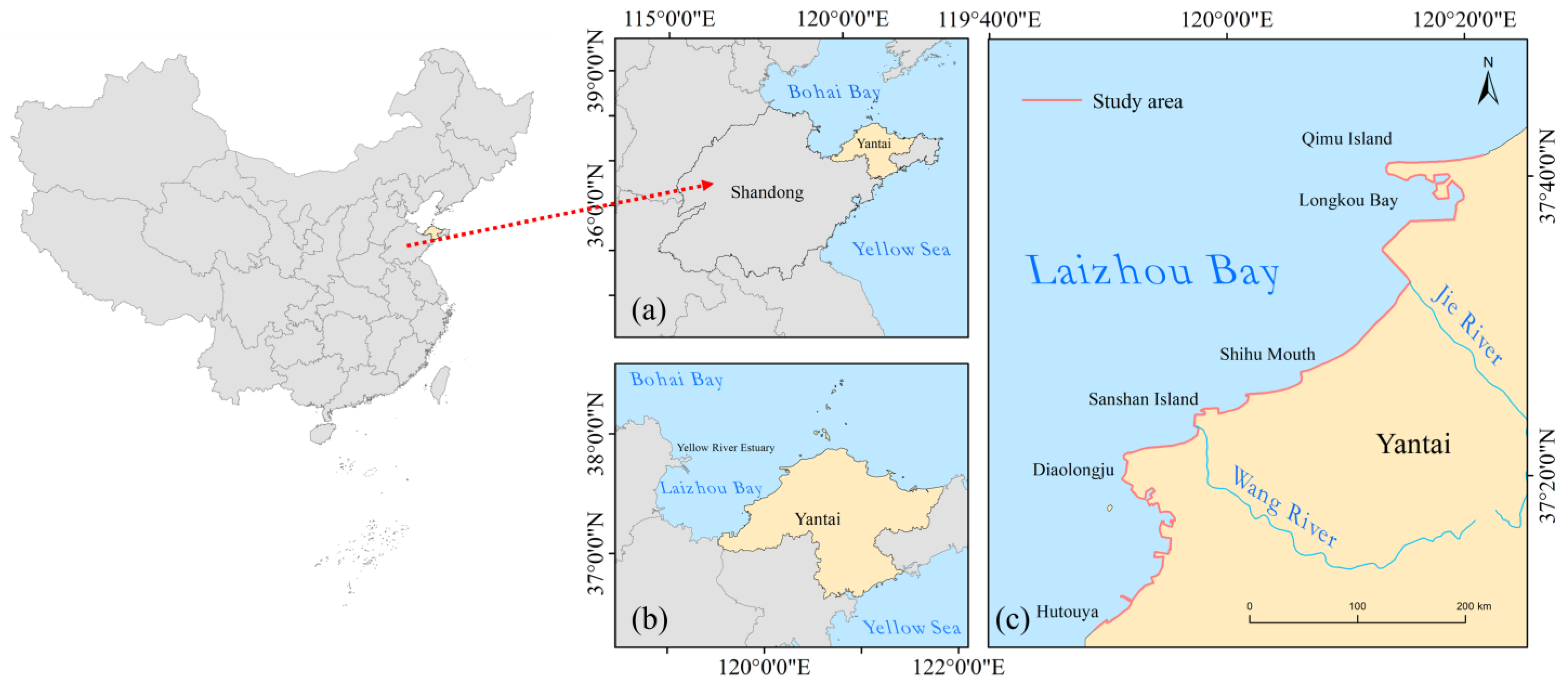
2.1. Study Area
2.2. Data Sources
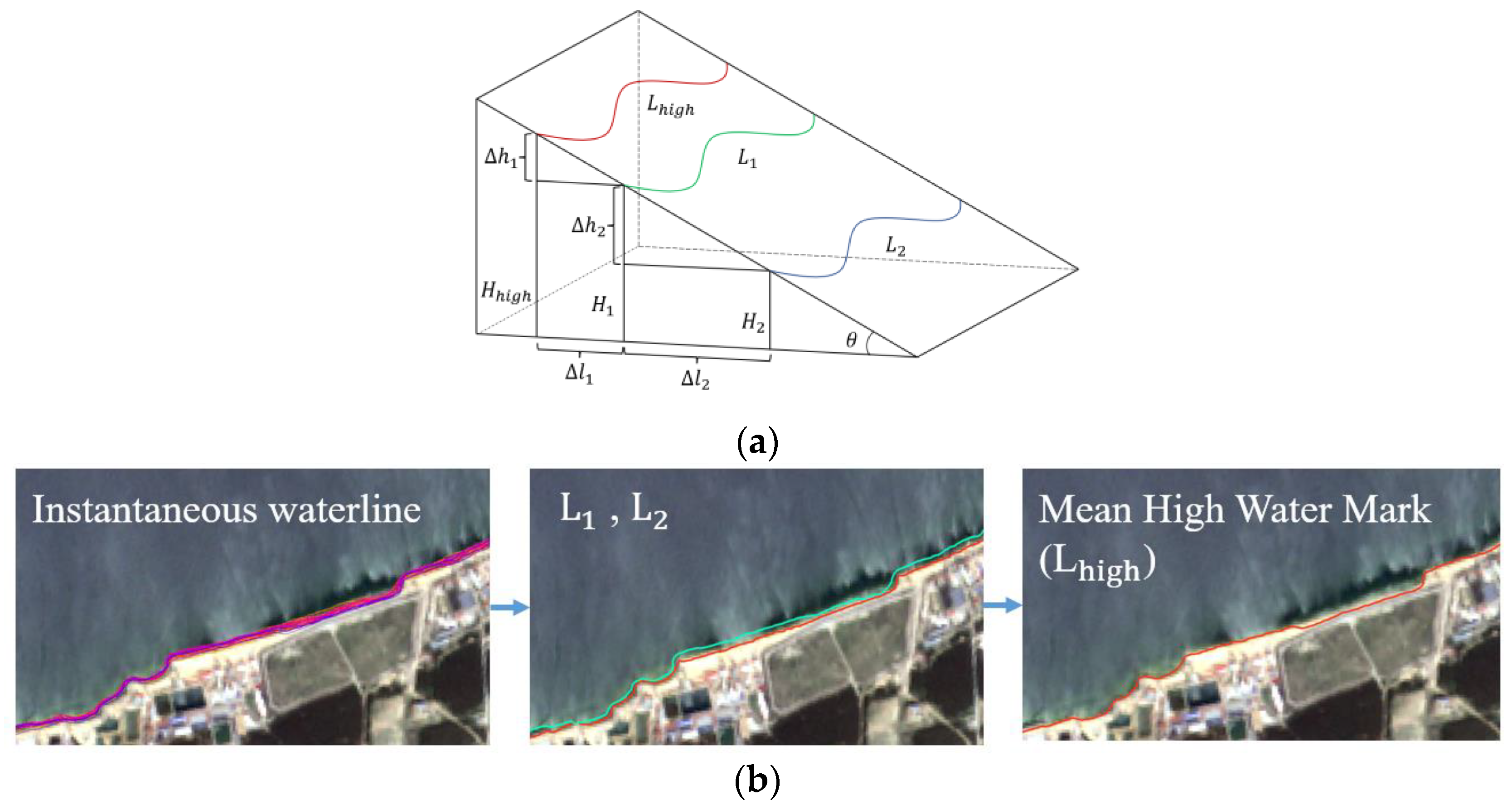
2.3. Extraction of the Coastline Position
2.4. Shoreline Classification
2.5. Coastline Diversity
2.6. Coastline Changes
2.7. Coastline Utilization
2.8. Coastline Complexity
2.9. Prediction of Shoreline Evolution
3. Results
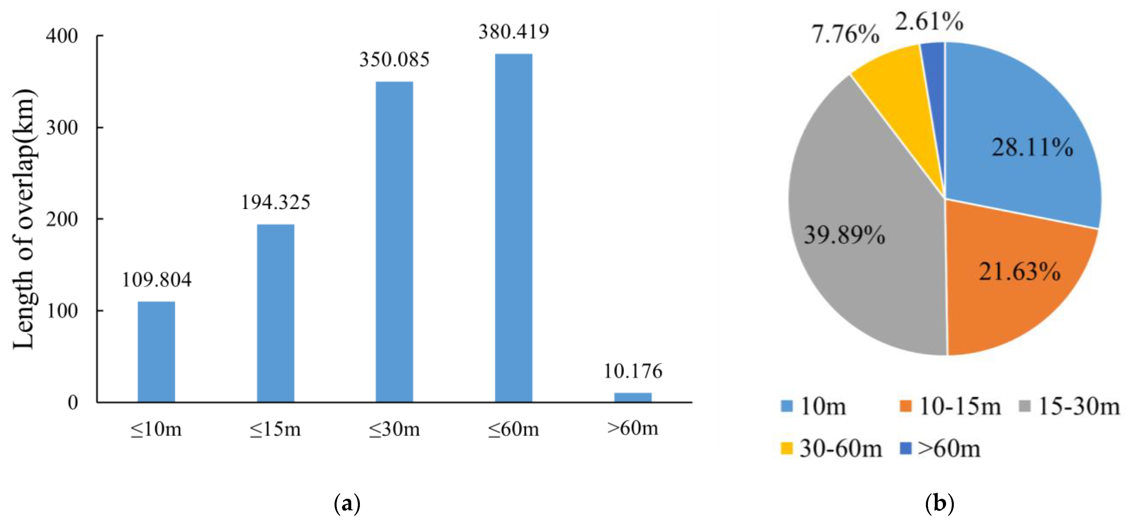
3.1. Coastline Accuracy Analysis
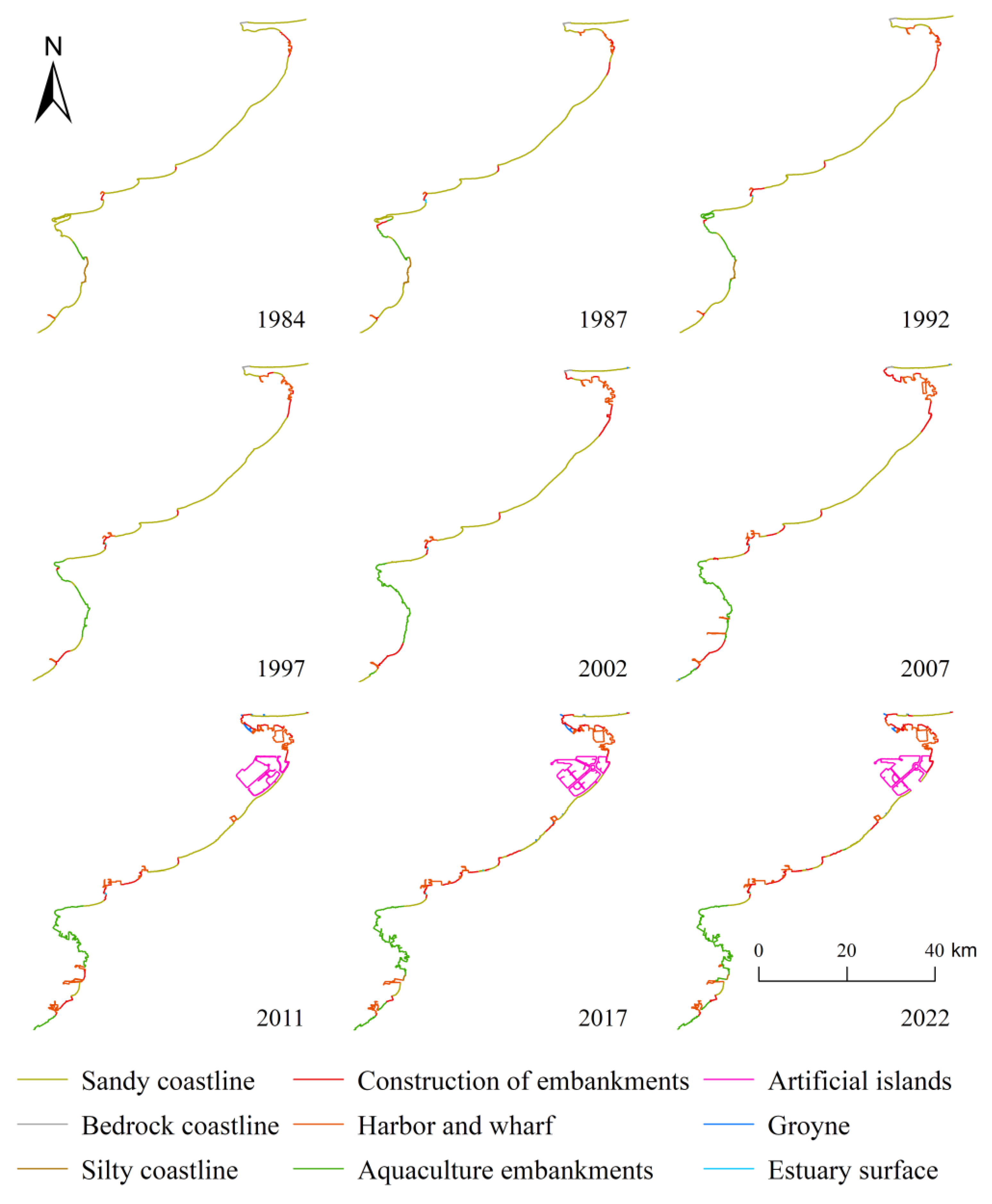
3.2. Analysis of Spatio-Temporal Changes in the Coastline
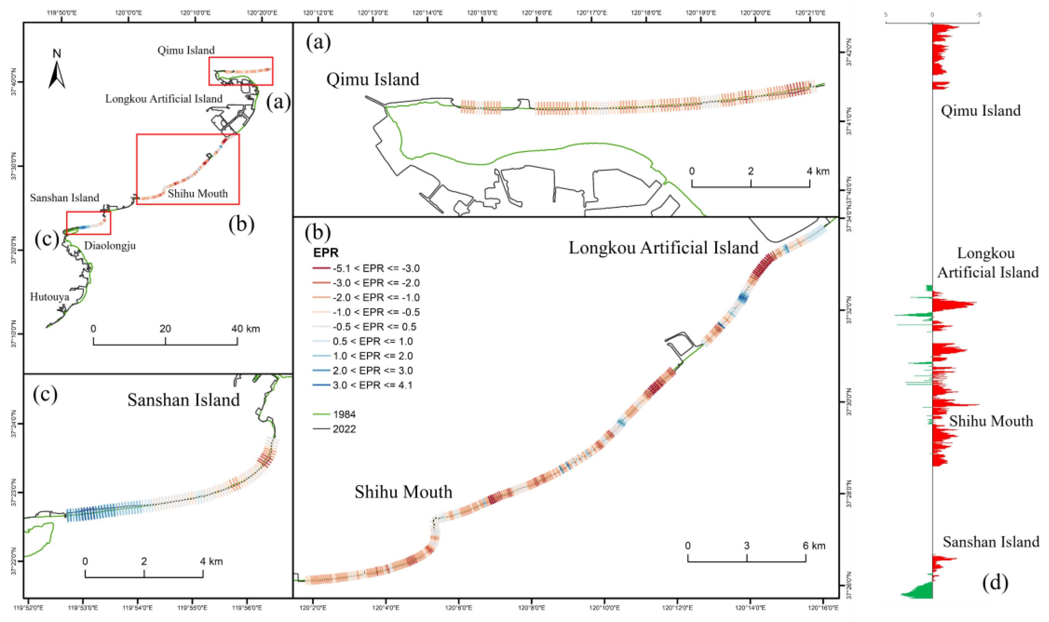
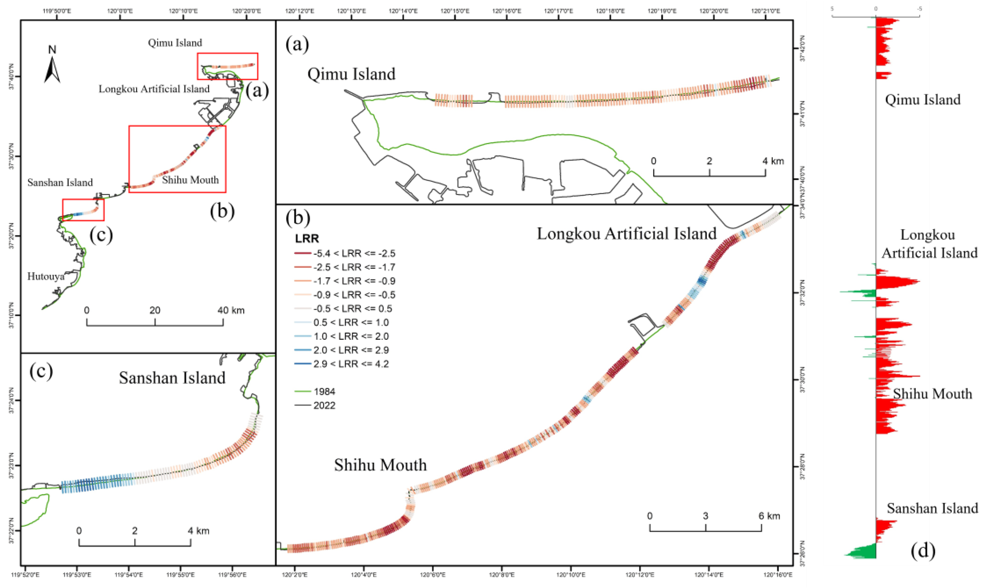
3.3. Analysis of Coastline Change Rate
3.4. Spatiotemporal Characteristics of the Fractal Dimension
3.5. Analysis of the Reasons for Coastline Changes
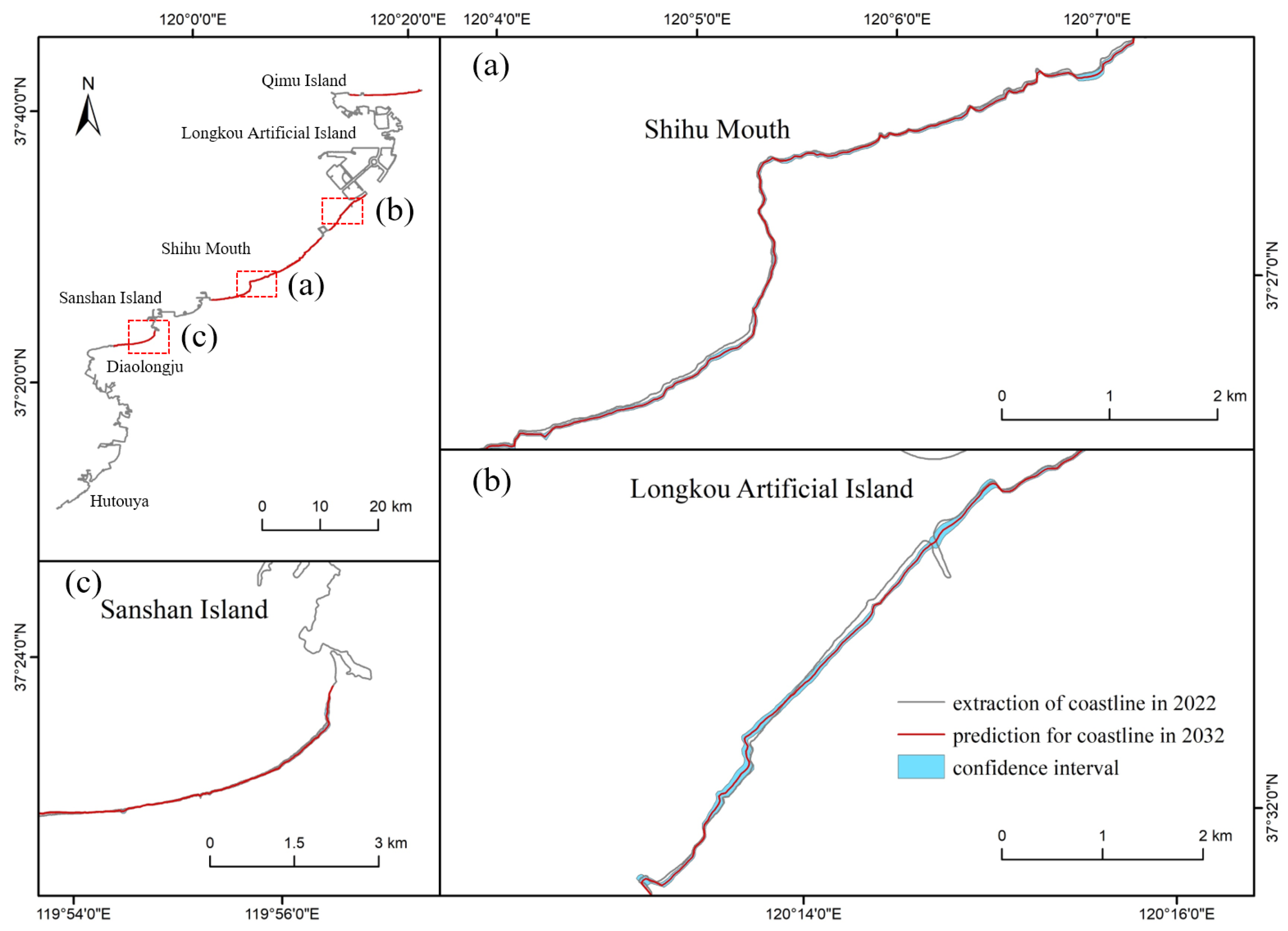
3.6. Prediction of Coastline Evolution
4. Discussion
5. Conclusions
- The coastal area expanded seaward by 12,025.42 hectares and eroded by 261.21 hectares, resulting in an increase in coastal length from 166.90 km to 364.20 km. All types of coasts were affected, although to varying degrees, both in terms of percentage distribution and over the different time periods analyzed.
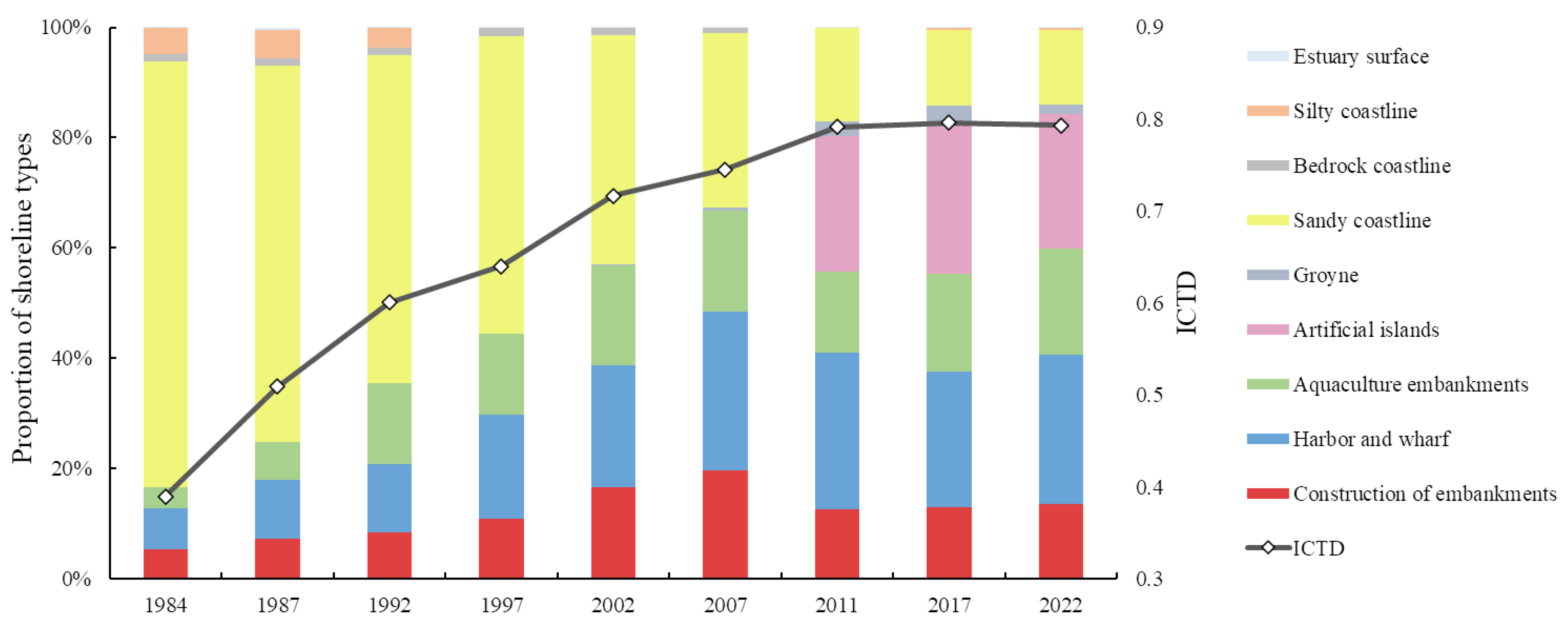
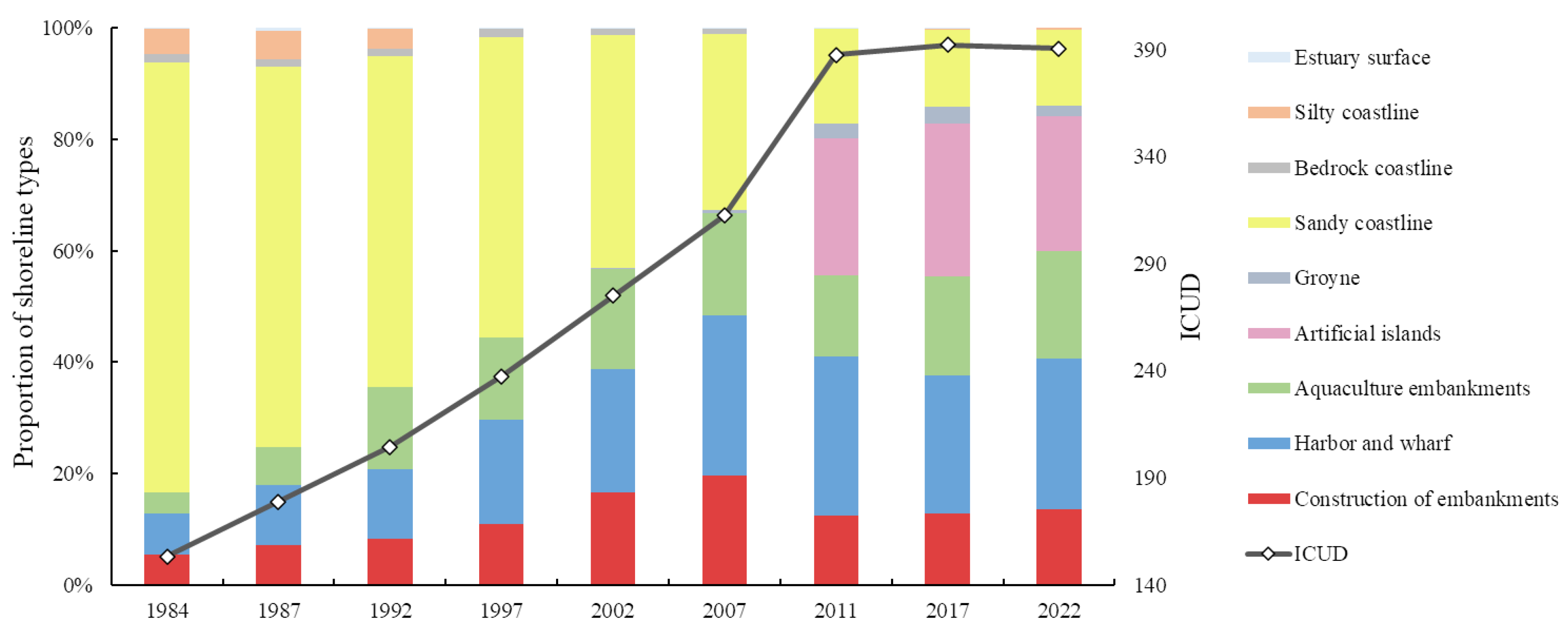
- The proportion of the natural coast continuously decreased leading to an increasing diversity of coastline types over the whole observation period.
- Coastline diversity and the intensity of the development of human activity show a consistent increase from 1984 to 2022, which was slow from 1984 to 2007 and fast between 2007 and 2011, while remaining relatively stable since 2011.
- The change in the intensity of the coastline between 1984 and 2022 is 3.11%. The highest value is 17.24% and relates to the period 2007–2011.
- The fractal dimension of the coastline showed an upward trend between 1984 and 2022. A positive correlation with the length of the coastline indicates the influence of human activities on the changes in the coastline.
- In the coastal erosion recorded in 2022, the proportion of sandy coastline erosion calculated by EPR is 79.54%, while the proportion calculated by LRR is 85.59%, which indicates a severe extent, especially in the central part, where natural factors and human intervention interact.
- The prediction of coastline evolution by 2023 shows that 84.58% of the sandy coastal sections will be affected by varying degrees of erosion, with the most severe condition being reached at a retreat rate of −2.53 . Conversely, only 15.32% of sandy beaches will increase due to sedimentation, with the progradation rate reaching 2.66 .
Author Contributions
Funding
Data Availability Statement
Acknowledgments
Conflicts of Interest
References
- Boak, E.H.; Turner, I.L. Shoreline Definition and Detection: A Review. J. Coast. Res. 2005, 21, 688–703. [Google Scholar] [CrossRef]
- Adu, K.; Emmanuel, M.A.; Kwaku, K.-K.; Osman, A. Socio—Economic Impact of Lake Bosomtwe Shoreline Changes on Catchment Residents in Ghana. Int. J. Sci. Res. Publ. 2014, 4, 1–7. [Google Scholar]
- Paterson, S.K.; O’Donnell, A.; Loomis, D.K.; Hom, P. The Social and Economic Effects of Shoreline Change: North Atlantic, South Atlantic, Gulf of Mexico, and Great Lakes Regional Overview; Eastern Research Group Inc: Lexington, MA, USA, 2010. [Google Scholar]
- Guimarais, M.; Zúñiga-Ríos, A.; Cruz-Ramírez, C.J.; Chávez, V.; Odériz, I.; Van Tussenbroek, B.I.; Silva, R. The Conservational State of Coastal Ecosystems on the Mexican Caribbean Coast: Environmental Guidelines for Their Management. Sustainability 2021, 13, 2738. [Google Scholar] [CrossRef]
- Moussa, M.; Baccar, L.; Ben Khemis, R. La lagune de Ghar El Melh: Diagnostic écologique et perspectives d’aménagement hydraulique. Rev. Sci. L’eau 2005, 18, 13–26. [Google Scholar] [CrossRef]
- Nichols, C.R.; Zinnert, J.; Young, D.R. Degradation of Coastal Ecosystems: Causes, Impacts and Mitigation Efforts. In Tomorrow’s Coasts Complex Impermanent; Springer: Cham, Switzerland, 2019; pp. 119–136. [Google Scholar]
- Lewin, W.-C.; Mehner, T.; Ritterbusch, D.; Brämick, U. The Influence of Anthropogenic Shoreline Changes on the Littoral Abundance of Fish Species in German Lowland Lakes Varying in Depth as Determined by Boosted Regression Trees. Hydrobiologia 2014, 724, 293–306. [Google Scholar] [CrossRef]
- Anderson, A.; Ratas, U.; Rivis, R.; Palginõmm, V. Relationship between Coastline Changes and Dynamics of Coastal Ecosystems of Tahkuna Peninsula, Estonia. In Proceedings of the 2012 IEEE/OES Baltic International Symposium (BALTIC), Klaipeda, Lithuania, 8–10 May 2012; pp. 1–6. [Google Scholar]
- Manyama, M.T.; Hepelwa, A.S.; Nahonyo, C.L. Analysis of Socio-Ecological Impacts of Built Environment at Dar Es Salaam Metropolitan Coastline, Tanzania. Open J. Soc. Sci. 2019, 07, 161–182. [Google Scholar] [CrossRef]
- Li, J.; Liu, Y.; Pu, R.; Yuan, Q.; Shi, X.; Guo, Q.; Song, X. Coastline and Landscape Changes in Bay Areas Caused by Human Activities: A Comparative Analysis of Xiangshan Bay, China and Tampa Bay, USA. J. Geogr. Sci. 2018, 28, 1127–1151. [Google Scholar] [CrossRef]
- Bailey, G.N.; King, G.C. Dynamic Landscapes and Human Dispersal Patterns: Tectonics, Coastlines, and the Reconstruction of Human Habitats. Quat. Sci. Rev. 2011, 30, 1533–1553. [Google Scholar] [CrossRef]
- Petrişor, A.-I.; Hamma, W.; Nguyen, H.D.; Randazzo, G.; Muzirafuti, A.; Stan, M.-I.; Tran, V.T.; Aştefănoaiei, R.; Bui, Q.-T.; Vintilă, D.-F. Degradation of Coastlines under the Pressure of Urbanization and Tourism: Evidence on the Change of Land Systems from Europe, Asia and Africa. Land 2020, 9, 275. [Google Scholar] [CrossRef]
- Appeaning Addo, K.; Jayson-Quashigah, P.N.; Kufogbe, K.S. Quantitative Analysis of Shoreline Change Using Medium Resolution Satellite Imagery in Keta, Ghana. Mar. Sci. 2012, 1, 1–9. [Google Scholar] [CrossRef]
- Cazenave, A.; Cozannet, G.L. Sea Level Rise and Its Coastal Impacts. Earth’s Future 2014, 2, 15–34. [Google Scholar] [CrossRef]
- Shalaby, A.; Tateishi, R. Remote Sensing and GIS for Mapping and Monitoring Land Cover and Land-Use Changes in the Northwestern Coastal Zone of Egypt. Appl. Geogr. 2007, 27, 28–41. [Google Scholar] [CrossRef]
- Muttitanon, W.; Tripathi, N.K. Land Use/Land Cover Changes in the Coastal Zone of Ban Don Bay, Thailand Using Landsat 5 TM Data. Int. J. Remote Sens. 2005, 26, 2311–2323. [Google Scholar] [CrossRef]
- Esteves, L.; Williams, J.; Nock, A.; Lymbery, G. Quantifying Shoreline Changes along the Sefton Coast (UK) and the Implications for Research-Informed Coastal Management. J. Coast. Res. 2009, 602–606. [Google Scholar]
- Cenci, L.; Disperati, L.; Persichillo, M.G.; Oliveira, E.R.; Alves, F.L.; Phillips, M. Integrating Remote Sensing and GIS Techniques for Monitoring and Modeling Shoreline Evolution to Support Coastal Risk Management. GISci. Remote Sens. 2018, 55, 355–375. [Google Scholar] [CrossRef]
- Mahrad, B.E.; Newton, A.; Icely, J.D.; Kacimi, I.; Abalansa, S.; Snoussi, M. Contribution of Remote Sensing Technologies to a Holistic Coastal and Marine Environmental Management Framework: A Review. Remote Sens. 2020, 12, 2313. [Google Scholar] [CrossRef]
- Lodato, F.; Colonna, N.; Pennazza, G.; Praticò, S.; Santonico, M.; Vollero, L.; Pollino, M. Analysis of the Spatiotemporal Urban Expansion of the Rome Coastline through GEE and RF Algorithm, Using Landsat Imagery. ISPRS Int. J. Geo-Inf. 2023, 12, 141. [Google Scholar] [CrossRef]
- Arjasakusuma, S.; Kusuma, S.S.; Saringatin, S.; Wicaksono, P.; Mutaqin, B.W.; Rafif, R. Shoreline Dynamics in East Java Province, Indonesia, from 2000 to 2019 Using Multi-Sensor Remote Sensing Data. Land 2021, 10, 100. [Google Scholar] [CrossRef]
- Ding, Y.; Yang, X.; Jin, H.; Wang, Z.; Liu, Y.; Liu, B.; Zhang, J.; Liu, X.; Gao, K.; Meng, D. Monitoring Coastline Changes of the Malay Islands Based on Google Earth Engine and Dense Time-Series Remote Sensing Images. Remote Sens. 2021, 13, 3842. [Google Scholar] [CrossRef]
- Maiti, S.; Bhattacharya, A.K. Shoreline Change Analysis and Its Application to Prediction: A Remote Sensing and Statistics Based Approach. Mar. Geol. 2009, 257, 11–23. [Google Scholar] [CrossRef]
- Hamzaoglu, C.; Dihkan, M. Automatic Extraction of Highly Risky Coastal Retreat Zones Using Google Earth Engine (GEE). Int. J. Environ. Sci. Technol. 2023, 20, 353–368. [Google Scholar] [CrossRef]
- Wang, X.; Xiao, X.; Zou, Z.; Chen, B.; Ma, J.; Dong, J.; Doughty, R.B.; Zhong, Q.; Qin, Y.; Dai, S. Tracking Annual Changes of Coastal Tidal Flats in China during 1986–2016 through Analyses of Landsat Images with Google Earth Engine. Remote Sens. Environ. 2020, 238, 110987. [Google Scholar] [CrossRef] [PubMed]
- Bishop-Taylor, R.; Nanson, R.; Sagar, S.; Lymburner, L. Mapping Australia’s Dynamic Coastline at Mean Sea Level Using Three Decades of Landsat Imagery. Remote Sens. Environ. 2021, 267, 112734. [Google Scholar] [CrossRef]
- Xu, Y.; Gao, H.; Wei, X.; Zhu, J. The Effects of Reclamation Activity and Yellow River Runoff on Coastline and Area of the Laizhou Bay, China. J. Ocean Univ. China 2021, 20, 729–739. [Google Scholar] [CrossRef]
- Liu, C.; Chang, J.; Chen, M.; Zhang, T. Dynamic Monitoring and Its Influencing Factors Analysis of Coastline in the Laizhou Bay since 1985. J. Coast. Res. 2020, 105, 18–22. [Google Scholar] [CrossRef]
- Jian, W.; Junqiang, Z.; Zhiqian, G.; Yameng, L.; Ying, G. Coastal Evolution of Southern Coast of Laizhou Bay during 1973–2016 and Maintanence Countermeasures. Mar. Geol. Front. 2019, 35, 27–36. [Google Scholar]
- Weifu, S.; Jie, Z.; Guangbo, R.; Yi, M.; Shaoqi, N. Coastline Remote Sensing Monitoring and Change Analysis of Laizhou Bay from 1978 to 2009; Atlantis Press: Amsterdam, The Netherlands, 2013; pp. 38–41. [Google Scholar]
- Kalman, R.E. A New Approach to Linear Filtering and Prediction Problems. J. Basic Eng. 1960, 82, 35–45. [Google Scholar] [CrossRef]
- Long, J.W.; Plant, N.G. Extended Kalman Filter Framework for Forecasting Shoreline Evolution. Geophys. Res. Lett. 2012, 39, L13603–L13608. [Google Scholar] [CrossRef]
- Vos, K.; Splinter, K.D.; Harley, M.D.; Simmons, J.A.; Turner, I.L. CoastSat: A Google Earth Engine-Enabled Python Toolkit to Extract Shorelines from Publicly Available Satellite Imagery. Environ. Model. Softw. 2019, 122, 104528. [Google Scholar] [CrossRef]
- Tu, T.-M.; Su, S.-C.; Shyu, H.-C.; Huang, P.S. A New Look at IHS-like Image Fusion Methods. Inf. Fusion 2001, 2, 177–186. [Google Scholar] [CrossRef]
- Xu, H. Modification of Normalised Difference Water Index (NDWI) to Enhance Open Water Features in Remotely Sensed Imagery. Int. J. Remote Sens. 2006, 27, 3025–3033. [Google Scholar] [CrossRef]
- Otsu, N. A Threshold Selection Method from Gray-Level Histograms. IEEE Trans. Syst. Man Cybern. 1979, 9, 62–66. [Google Scholar] [CrossRef]
- Cipolletti, M.P.; Delrieux, C.A.; Perillo, G.M.E.; Cintia Piccolo, M. Superresolution Border Segmentation and Measurement in Remote Sensing Images. Comput. Geosci. 2012, 40, 87–96. [Google Scholar] [CrossRef]
- Carrere, L.; Lyard, F.; Cancet, M.; Guillot, A. FES 2014, a New Tidal Model on the Global Ocean with Enhanced Accuracy in Shallow Seas and in the Arctic Region. In Proceedings of the EGU General Assembly Conference Abstracts, Vienna, Austria, 12–17 April 2015; p. 5481. [Google Scholar]
- Wu, T. Analysis of Spatio-Temporal Characteristics of Mainland Coastline Changes in China in Nearly 70 Years. Ph.D. Thesis, Yantai Institute of Coastal Zone Research, Chinese Academy of Sciences, Beijing, China, 2016. (In Chinese). [Google Scholar]
- Xu, J.; Zhang, Z.; Zhao, X.; Wen, Q.; Zuo, L.; Wang, X.; Yi, L. Spatial-temporal analysis of coastline changes in northern China from 2000 to 2012. Acta Geogr. Sin. 2013, 68, 651–660. (In Chinese) [Google Scholar]
- Dolan, R.; Fenster, M.S. Temporal Analysis of Shoreline Recession and Accretion. J. Coast. Res. 1991, 7, 723–744. [Google Scholar]
- Zeinali, S.; Talebbeydokhti, N.; Dehghani, M. Spatiotemporal Shoreline Change in Boushehr Province Coasts, Iran. J. Ocean Limnol. 2020, 38, 707–721. [Google Scholar] [CrossRef]
- Himmelstoss, E.A.; Henderson, R.E.; Kratzmann, M.G.; Farris, A.S. Digital Shoreline Analysis System (DSAS) Version 5.0 User Guide; US Geological Survey: Reston, VA, USA, 2018. [Google Scholar] [CrossRef]
- Wu, T.; Hou, X.; Xu, X. Spatio-Temporal Characteristics of the Mainland Coastline Utilization Degree over the Last 70 Years in China. Ocean Coast. Manag. 2014, 98, 150–157. [Google Scholar] [CrossRef]
- Mandelbrot, B. How Long Is the Coast of Britain? Statistical Self-Similarity and Fractional Dimension. Science 1967, 156, 636–638. [Google Scholar] [CrossRef] [PubMed]
- Ludeman, L.C. Random Processes: Filtering, Estimation, and Detection; John Wiley & Sons, Inc.: Hoboken, NJ, USA, 2003; ISBN 0-471-25975-6. [Google Scholar]
- Liu, C.; Shi, R.X.; Zhang, Y.H.; Shen, Y.; Ma, J.H.; Wu, L.Z.; Doko, T.; Chen, L.J.; Lv, T.T.; Tao, Z.; et al. 2015: How Many Islands (Isles, Rocks), How Large Land Areas and How Long of Shorelines in the World?—Vector Data Based on Google Earth Images. J. Glob. Change Data Discov. 2019, 3, 124–148. [Google Scholar]
- Sun, Y.; Xu, S.; Wang, Q.; Hu, S.; Qin, G.; Yu, H. Response of a Coastal Groundwater System to Natural and Anthropogenic Factors: Case Study on East Coast of Laizhou Bay, China. Int. J. Environ. Res. Public Health. 2020, 17, 5204. [Google Scholar] [CrossRef]
- Gao, X.; Zhuang, W.; Chen, C.-T.A.; Zhang, Y. Sediment Quality of the SW Coastal Laizhou Bay, Bohai Sea, China: A Comprehensive Assessment Based on the Analysis of Heavy Metals. PLoS ONE 2015, 10, e0122190. [Google Scholar] [CrossRef] [PubMed]
- Donnici, S.; Serandrei-Barbero, R.; Gao, X.; Tang, C.; Tosi, L. Utilizing Benthic Foraminifera to Explore the Environmental Condition of the Laizhou Bay (Bohai Sea, China). Mar. Pollut. Bull. 2021, 167, 112323. [Google Scholar] [CrossRef] [PubMed]
- Yu, X.; Wang, Z.; Leng, X.; Liu, D.; Yang, X.; Zhang, Q.; Li, A. Effects of Mariculture on Hydrodynamic Conditions in Laizhou Bay. Period. Ocean. Univ. China 2022, 52, 132–139. (In Chinese) [Google Scholar] [CrossRef]
- Tian, B.; Wu, W.; Yang, Z.; Zhou, Y. Drivers, Trends, and Potential Impacts of Long-Term Coastal Reclamation in China from 1985 to 2010. Estuar. Coast. Shelf Sci. 2016, 170, 83–90. [Google Scholar] [CrossRef]
- Gong, M.; Wu, X.; Yu, L. Reclamation Dynamics Along the Mainland Coast of Shandong Province during 1974–2017. J. Geo-Inf. Sci. 2019, 21, 1911–1922. (In Chinese) [Google Scholar] [CrossRef]
- Zhan, C.; Yu, J.; Wang, Q.; Su, Y.; Zhou, D. Spatial and Temporal Dynamics of Sandy Coastal Geomorphlogy in The East of Laizhou Bay Over Recent 60 Years. Acta Oceanol. Sin. 2017, 39, 90–100. (In Chinese) [Google Scholar] [CrossRef]
- Zhuang, Z.; Lin, Z.; Liu, Z.; Deng, X. Sea Level Changes and Coastal Responses. Mar. Geol. Lett. 2003, 19, 1–12. (In Chinese) [Google Scholar] [CrossRef]
- Leatherman, S.P.; Zhang, K.; Douglas, B.C. Sea Level Rise Shown to Drive Coastal Erosion. Eos Trans. Am. Geophys. Union 2000, 81, 55–57. [Google Scholar] [CrossRef]
- Peng, M.; Zhao, C.; Zhang, Q.; Lu, Z.; Bai, L.; Bai, W. Multi-Scale and Multi-Dimensional Time Series InSAR Characterizing of Surface Deformation over Shandong Peninsula, China. Appl. Sci. 2020, 10, 2294. [Google Scholar] [CrossRef]
- Quanyuan, W.; Jiewu, P.; Shanzhong, Q.; Yiping, L.; Congcong, H.; Tingxiang, L.; Limei, H. Impacts of Coal Mining Subsidence on the Surface Landscape in Longkou City, Shandong Province of China. Environ. Earth Sci. 2009, 59, 783–791. [Google Scholar] [CrossRef]
- Liu, K.-X.; Wang, H.; Fu, S.-J.; Gao, Z.-G.; Dong, J.-X.; Feng, J.-L.; Gao, T. Evaluation of Sea Level Rise in Bohai Bay and Associated Responses. Adv. Clim. Change Res. 2017, 8, 48–56. [Google Scholar] [CrossRef]
- Li, Y.; Zhang, H.; Tang, C.; Zou, T.; Jiang, D. Influence of Rising Sea Level on Tidal Dynamics in the Bohai Sea. J. Coast. Res. 2016, 74, 22–31. [Google Scholar] [CrossRef]
- Harris, L.R.; Bessinger, M.; Dayaram, A.; Holness, S.; Kirkman, S.; Livingstone, T.-C.; Lombard, A.T.; Lück-Vogel, M.; Pfaff, M.; Sink, K.J.; et al. Advancing Land-Sea Integration for Ecologically Meaningful Coastal Conservation and Management. Biol. Conserv. 2019, 237, 81–89. [Google Scholar] [CrossRef]
- Annis, G.M.; Pearsall, D.R.; Kahl, K.J.; Washburn, E.L.; May, C.A.; Franks Taylor, R.; Cole, J.B.; Ewert, D.N.; Game, E.T.; Doran, P.J. Designing Coastal Conservation to Deliver Ecosystem and Human Well-Being Benefits. PLoS ONE 2017, 12, e0172458. [Google Scholar] [CrossRef] [PubMed]


| Primary Classification | Secondary Classification | Intensity Index |
|---|---|---|
| natural coastline | sandy coastline | 1 |
| bedrock coastline | 1 | |
| silty coastline | 1 | |
| artificial coastline | construction of embankments | 4 |
| harbor and wharf | 5 | |
| aquaculture embankments | 3 | |
| groynes | 4 | |
| artificial islands | 5 | |
| estuarine coastline | estuary surface | 2 |
| Time Period | LCI/% | |||||||||
|---|---|---|---|---|---|---|---|---|---|---|
| All Shorelines | Aquaculture Embankments | Construction of Embankments | Harbor and Wharf | Estuary Surface | Sandy Coastline | Silty Coastline | Bedrock Coastline | Groyne | Artificial Islands | |
| 1984–1987 | 0.45 | 27.68 | 11.36 | 16.34 | 120.29 | −3.48 | 3.40 | −1.02 | ||
| 1987–1992 | −0.31 | 22.32 | 2.71 | 2.97 | −17.27 | −2.87 | −5.86 | 0.33 | ||
| 1992–1997 | 0.25 | 0.46 | 6.49 | 10.33 | −4.48 | −1.64 | −20.00 | 3.50 | ||
| 1997–2002 | 1.66 | 6.45 | 12.96 | 5.56 | 28.10 | −3.25 | −2.81 | |||
| 2002–2007 | 2.71 | 3.23 | 6.90 | 9.42 | −5.89 | −2.83 | −0.92 | 58.68 | ||
| 2007–2011 | 17.24 | 8.3 | 1.95 | 16.96 | 41.33 | −2.22 | −25.00 | 183.76 | ||
| 2011–2017 | 1.78 | 5.77 | 2.38 | −0.70 | −9.37 | −1.80 | 5.36 | 3.85 | ||
| 2017–2022 | −1.21 | 0.44 | −0.22 | 0.53 | −12.28 | −1.47 | −0.03 | −8.86 | −3.29 | |
| 1984–2022 | 3.11 | 26.73 | 11.70 | 18.56 | −1.65 | −1.63 | −2.17 | |||
| Time Period | Number of Profiles | ) | ) | Unchanged | |||||||||
|---|---|---|---|---|---|---|---|---|---|---|---|---|---|
| Maximum | Average | Median | Standard Deviation | Proportion/% | Minimum Value | Average | Median | Standard Deviation | Proportion/% | Proportion/% | |||
| EPR | 1984–1987 | 933 | 27.22 | 8.11 | 7.35 | 5.26 | 71.28 | −21.46 | −6.94 | −6.05 | 4.83 | 28.72 | 0.00 |
| 1987–1992 | 893 | 21.69 | 6.13 | 4.30 | 5.07 | 39.87 | −18.81 | −5.09 | −4.43 | 3.66 | 59.80 | 0.33 | |
| 1992–1997 | 820 | 36.39 | 5.00 | 3.67 | 5.00 | 57.07 | −14.03 | −3.21 | −2.49 | 2.68 | 42.93 | 0.00 | |
| 1997–2002 | 691 | 27.80 | 3.62 | 2.19 | 5.03 | 20.12 | −26.63 | −4.48 | −3.88 | 3.21 | 79.88 | 0.00 | |
| 2002–2007 | 634 | 8.61 | 2.11 | 1.69 | 1.66 | 36.75 | −15.42 | −3.39 | −3.00 | 2.63 | 63.25 | 0.00 | |
| 2007–2011 | 497 | 14.76 | 2.77 | 2.16 | 2.71 | 23.34 | −29.25 | −6.09 | −4.77 | 5.28 | 76.66 | 0.00 | |
| 2011–2017 | 476 | 25.85 | 3.71 | 2.43 | 4.12 | 25.84 | −19.3 | −4.94 | −4.54 | 3.36 | 74.16 | 0.00 | |
| 2017–2022 | 504 | 27.71 | 2.63 | 2.10 | 2.27 | 74.00 | −6.02 | −1.64 | −1.25 | 1.45 | 25.60 | 0.40 | |
| 1984–2022 | 513 | 4.05 | 1.20 | 0.71 | 1.05 | 20.08 | −5.06 | −1.34 | −1.19 | 0.89 | 79.54 | 0.38 | |
| LRR | 1984–2022 | 513 | 4.13 | 1.50 | 1.33 | 1.10 | 14.42 | −5.34 | −1.56 | −1.4 | 1.00 | 85.58 | 0.00 |
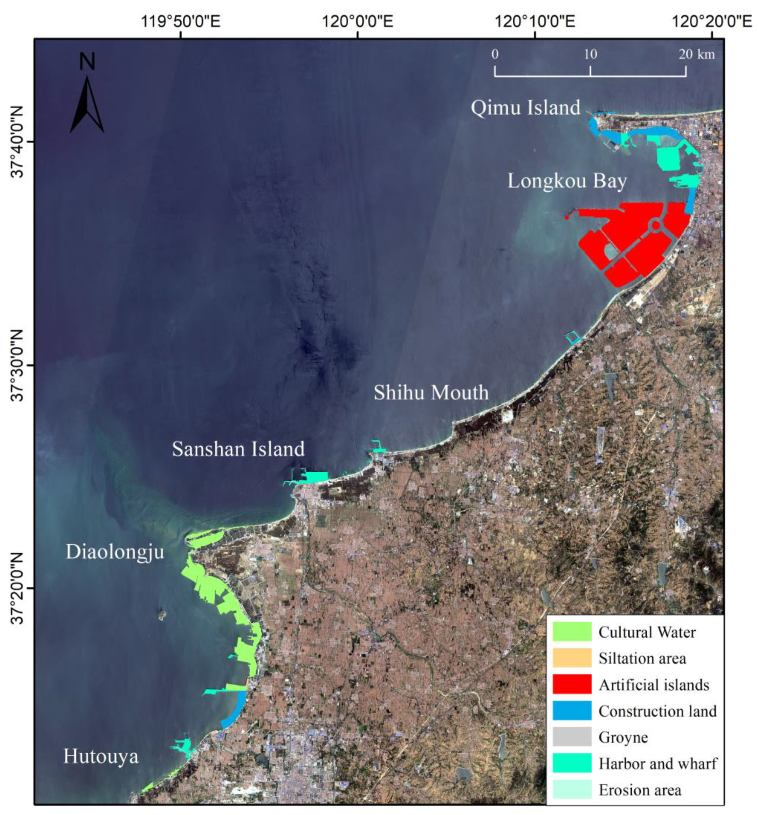
| Type | Human Activities | Natural Activities | |||||
|---|---|---|---|---|---|---|---|
| Artificial Islands | Aquaculture Water Bodies | Harbor and Wharf | Construction Land | Groyne | Erosion | Accumulation | |
| area/ha | 5802.73 | 2846.27 | 1985.63 | 1351.20 | 49.67 | 261.21 | 39.60 |
| percentage/% | 47.04 | 23.07 | 16.10 | 10.95 | 0.40 | 2.12 | 0.32 |
Disclaimer/Publisher’s Note: The statements, opinions and data contained in all publications are solely those of the individual author(s) and contributor(s) and not of MDPI and/or the editor(s). MDPI and/or the editor(s) disclaim responsibility for any injury to people or property resulting from any ideas, methods, instructions or products referred to in the content. |
© 2024 by the authors. Licensee MDPI, Basel, Switzerland. This article is an open access article distributed under the terms and conditions of the Creative Commons Attribution (CC BY) license (https://creativecommons.org/licenses/by/4.0/).
Share and Cite
Mu, K.; Tang, C.; Tosi, L.; Li, Y.; Zheng, X.; Donnici, S.; Sun, J.; Liu, J.; Gao, X. Coastline Monitoring and Prediction Based on Long-Term Remote Sensing Data—A Case Study of the Eastern Coast of Laizhou Bay, China. Remote Sens. 2024, 16, 185. https://doi.org/10.3390/rs16010185
Mu K, Tang C, Tosi L, Li Y, Zheng X, Donnici S, Sun J, Liu J, Gao X. Coastline Monitoring and Prediction Based on Long-Term Remote Sensing Data—A Case Study of the Eastern Coast of Laizhou Bay, China. Remote Sensing. 2024; 16(1):185. https://doi.org/10.3390/rs16010185
Chicago/Turabian StyleMu, Ke, Cheng Tang, Luigi Tosi, Yanfang Li, Xiangyang Zheng, Sandra Donnici, Jixiang Sun, Jun Liu, and Xuelu Gao. 2024. "Coastline Monitoring and Prediction Based on Long-Term Remote Sensing Data—A Case Study of the Eastern Coast of Laizhou Bay, China" Remote Sensing 16, no. 1: 185. https://doi.org/10.3390/rs16010185
APA StyleMu, K., Tang, C., Tosi, L., Li, Y., Zheng, X., Donnici, S., Sun, J., Liu, J., & Gao, X. (2024). Coastline Monitoring and Prediction Based on Long-Term Remote Sensing Data—A Case Study of the Eastern Coast of Laizhou Bay, China. Remote Sensing, 16(1), 185. https://doi.org/10.3390/rs16010185