Abstract
In this paper, a compound-Gaussian model (CGM) with the Nakagami-distributed textures (CGNG) is proposed to model sea clutter at medium/high grazing angles. The corresponding amplitude distributions are referred to as the CGNG distributions. The analysis of measured data shows that the CGNG distributions can provide better goodness-of-the-fit to sea clutter at medium/high grazing angles than the four types of commonly used biparametric distributions. As a new type of amplitude distribution, its parameter estimation is important for modelling sea clutter. The estimators from the method of moments (MoM) and the [zlog(z)] estimator from the method of generalized moments are first given for the CGNG distributions. However, these estimators are sensitive to sporadic outliers of large amplitude in the data. As the second contribution of the paper, outlier-robust tri-percentile estimators of the CGNG distributions are proposed. Moreover, experimental results using simulated and measured sea clutter data are reported to show the suitability of the CGNG amplitude distributions and outlier-robustness of the proposed tri-percentile estimators.
1. Introduction
Sea clutter modelling is of great significance for design and target detection of maritime radar [1,2,3,4,5,6] and target detection in high-resolution SAR images of oceanic scenes [7,8,9,10]. CGMs with different types of texture distributions have been used to model sea clutter at low grazing angles [11,12]. The famous biparametric distributions include the K-distributions [13], generalized Pareto distributions [14], CGIG distributions [15], and CGLN distributions [16]. Their textures follow the Gamma, inverse Gamma, inverse Gaussian, and lognormal distributions, respectively. In addition, a new type of biparametric distribution, the CIER distribution, is proposed and fits to some measured data well [17]. Triparametric distributions are also used to model non-Gaussian sea clutter, such as CG-GIG distributions [18] and generalized K distributions [19], and the corresponding textures follow the generalized inverse Gaussian distributions and the generalized Gamma distributions, respectively. The outlier-robust parameter estimation of the triparametric distributions is rather difficult. When the power parameter of the generalized K distributions is two, the generalized K distributions degenerate to the Nakagami distributions. In this paper, we introduce a new type of biparametric distributions, the CGM with the Nakagami-distributed textures (CGNG). Like the four types of commonly used texture distributions, the Nakagami distributions are a famous type of biparametric distribution used to characterize positive random variables [20]. At present, the optimal type selection of sea clutter amplitude distributions is based on statistical analysis of big data [21] instead of the physical scattering mechanism of the sea surface due to there being too many and complicated factors. In fact, various types of amplitude distributions are complementary so as to subtly model sea clutter in different conditions in a wide selectable space. By analyzing a Ku-band airborne high-resolution sea clutter database at medium/high grazing angles, it is found that the K-distributions, generalized Pareto distributions, CGIG distributions, and CGLN distributions do not always fit the amplitude distributions of the data well, and the CGNG distributions can better fit the Ku-band airborne high-resolution sea clutter data at medium/high grazing angles.
Sea clutter modelling includes both model construction and parameter estimation [22,23]. The estimators from the method of moments (MoM) and the [zlog(z)] estimator from the method of generalized moments are first given for the CGNG distributions. In cluttered environments of maritime radars, the received radar echoes inevitably contain a fraction of outliers from boats, reefs, or other strong scatterers on the sea surface [24,25]. It is difficult to cleanly exclude outliers before parameter estimation. It is difficult for the MoM estimators [14,26,27,28,29,30] and [zlog(z)] estimator [14,27,29,31] to provide robust parameter estimation in real clutter environments due to their sensitivity to outliers of large amplitudes. For other types of amplitude distributions, a series of outlier-robust percentile-based estimators, namely truncated maximum likelihood (TML) estimators or estimators based on the neural networks and multi-sample percentiles, have been developed in succession [32,33,34,35,36,37,38,39]. Like the CGLN distributions [27], the CGNG distributions lack analytical expressions, and thus it is difficult to derive the ML and TML estimates of the parameters.
Inspired by the outlier-robust tri-percentile estimators of CGLN distributions and K-distributions [32,36], the outlier-robust tri-percentile estimators of the CGNG distributions are constructed in this paper. First, we determine that the ratio of the two percentiles is free of the scale parameter and show that the ratio is a monotonic function of the inverse shape parameter via numerical computation. Second, for the given positions of two percentiles, we sort the sea clutter amplitude sequence in ascending order, and the ratio of the two sample percentiles is determined. Then, the estimate of the inverse shape parameter can be quickly obtained from the ratio using the look-up table method. Third, the scale parameter estimate can be obtained from the third sample percentile whose position is determined by the estimate of the inverse shape parameter. Obviously, the estimation performance depends on the selection of three percentile positions. From numerical computation and the asymptotic property of the sample percentile [40], the three optimal percentile positions are determined. Moreover, sea clutter data collected by an airborne Ku-band high-resolution radar are used to verify the suitability of the CGNG distributions and the outlier-robust tri-percentile estimators are assessed and compared using simulated and measured data.
The main novelties and contributions of the paper are shown below:
- A new CGM with Nakagami-distributed textures is proposed to model sea clutter at medium/high grazing angles. As the grazing angles increase, sea clutter becomes less spiky, i.e., sea clutter has a slighter tail. We compare the tail of the CGNG distributions with that of the K distributions, generalized Pareto distributions, CGIG distributions, and CGLN distributions and find the tails of the CGNG distributions are the slightest. Therefore, the CGNG distributions are proposed to model sea clutter at medium/high grazing angles.
- Sea clutter data inevitably contain a fraction of outliers. In order to achieve the robust parameter estimation of the CGNG distributions, the tri-percentile estimators are proposed.
This paper is organized as follows. Section 2 introduces the CGNG distributions and the motivation for using the CGNG distributions to model sea clutter at medium/high grazing angles, and gives the MoM estimators and [zlog(z)] estimator. Section 3 proposes the outlier-robust tri-percentile estimators of the CGNG distributions. Section 4 validates the suitability of the CGNG distributions to high-resolution sea clutter at medium/high grazing angles and verifies the outlier-robustness of the proposed tri-percentile estimators. Finally, Section 5 concludes our paper.
2. Compound-Gaussian Model with Nakagami-Distributed Textures
CGMs have been widely used in sea clutter modeling. In a CGM, sea clutter can be represented by two independent components, a fast-varying Gaussian speckle component and a slow-varying texture component [41]. The sea clutter sequence can be simply expressed as [13]
where n represents the pulse number; τ(n) is a slowly varying texture sequence, that is, a positive random sequence following different probability distributions; and u(n) is a complex Gaussian speckle sequence with zero mean and unit variance that conveys the Doppler spectral characteristics of sea clutter. The texture distributions reflect the power change of the sea clutter and non-Gaussianity. The biparametric Gamma, inverse Gamma, inverse Gaussian, and lognormal distributions have been used to model textures so as to adapt sea clutter data from various conditions. For some high-resolution sea clutter data at medium/high grazing angles, it is found that the four types of distributions fail to fit well. Therefore, we attempt to use the biparametric Nakagami distributions [20] to model textures in sea clutter instead of the four commonly used types of biparametric distributions. In order for the shape parameter to better reflect the tail thickness of textures, the Nakagami distributions are expressed as follows:
where υ and b are the shape and scale parameters, respectively, and b is equal to the clutter average power. In (2), we use the inverse shape parameter λ so as to highlight the refined characterization of non-Gaussianity. The clutter converges to complex Gaussian clutter when λ tends to zero and the clutter becomes spikier as λ tends to infinity.
In terms of the conditional probability formula, the amplitude of sea clutter follows the following probability density function (PDF) and the cumulative distribution function (CDF):
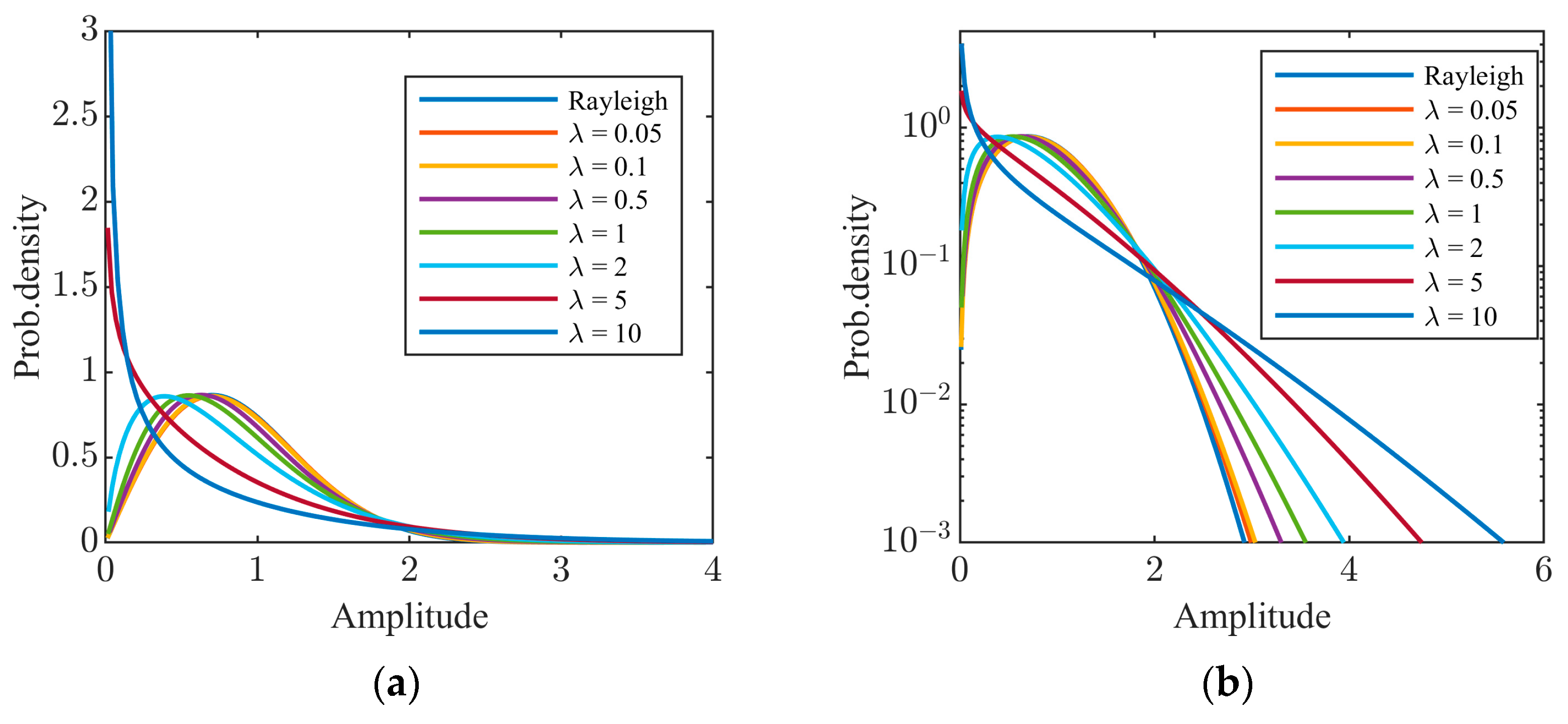
The biparametric distributions in (3) are referred to as the CGNG distributions. The inverse shape parameter λ reflects the non-Gaussianity of sea clutter. Figure 1 illustrates the main parts and tail parts of the CGNG distributions when the scale parameter b is fixed at 1 and the inverse shape parameter λ takes different values. It can be found that the larger λ is, the stronger the non-Gaussianity of the sea clutter is and the heavier the tail of the sea clutter is. On the contrary, the non-Gaussianity of the sea clutter becomes weaker when λ becomes smaller, and the CGNG distributions approximate to the Rayleigh distributions as λ tends to zero. Its proof is given as follows:
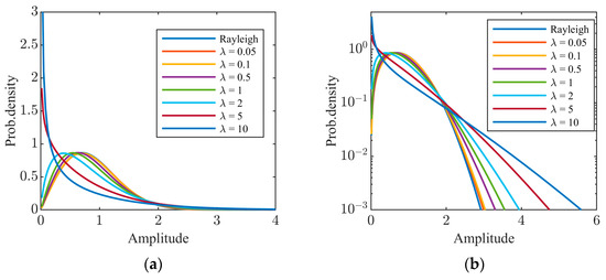
Figure 1.
CGNG distributions with different values of λ: (a) main parts; (b) tail parts.
The proof is straightforward by using Stirling’s approximation [42,43]. Therefore, the limit distribution of the CGNG distributions when λ tends to zero is the Rayleigh distribution.
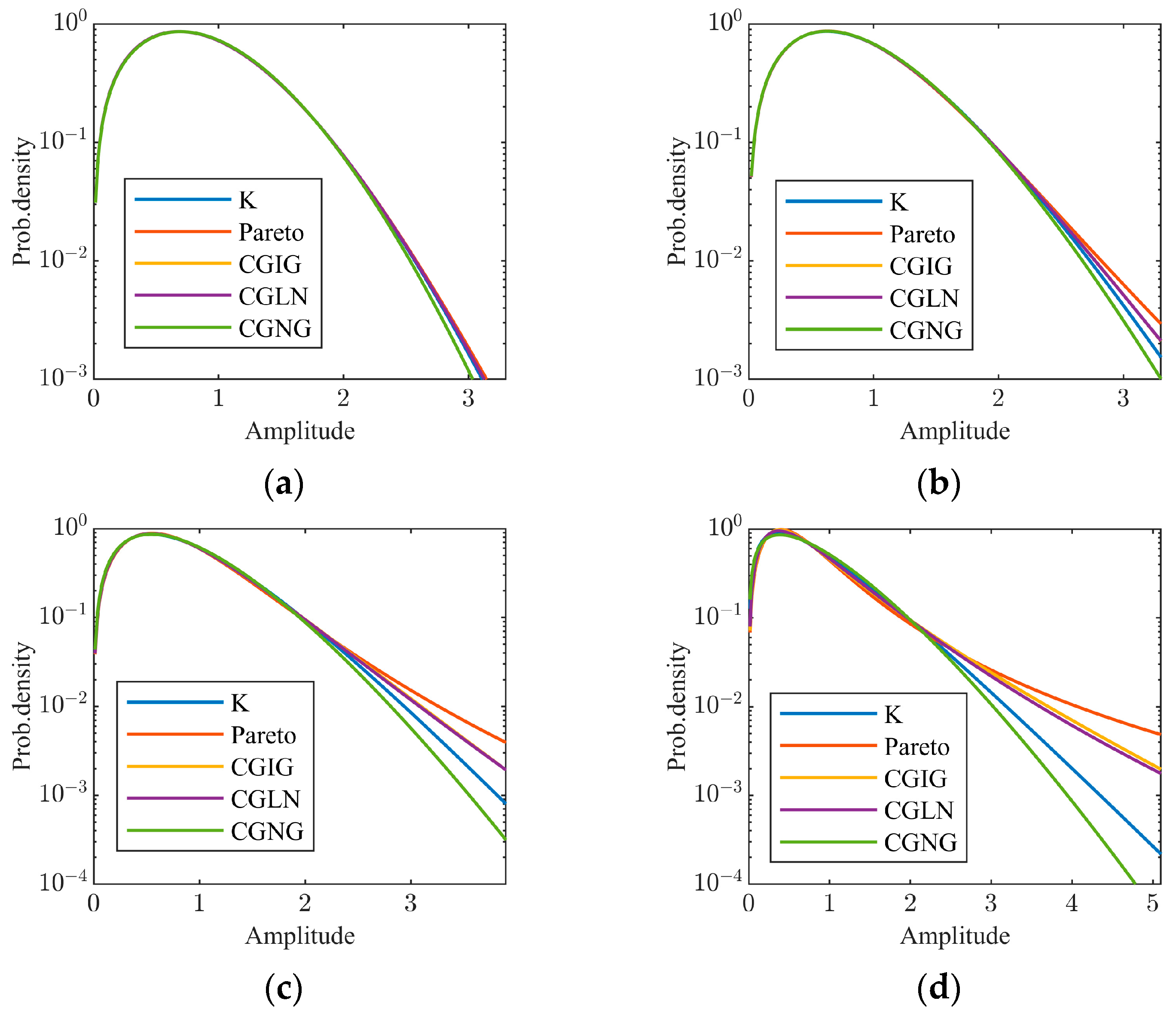
In order to show the necessity of the CGNG distributions in sea clutter modelling when the K distributions, generalized Pareto distributions, CGIG distributions, and CGLN distributions exist, we plot the tail parts of the CGNG distributions and the most approximate distributions under the four existing types in the sense of the Kolmogorov–Smirnov distance (KSD) [44] in the four different cases when the scale parameter of the CGNG distributions is b = 1 and the inverse shape parameter is 0.1, 0.5, 1, and 2, respectively. For each CGNG distribution, the values of the parameters of the four most approximate distributions and their KSDs from the CGNG distribution are listed in Table 1. It can be found that the maximal KSD at all the cases is very small and only 0.0390, meaning that the main parts of the most approximate distributions are sufficiently close to that of the CGNG distributions. As shown in Figure 2, the non-Gaussianity of the CGNG distributions becomes stronger from Figure 2a–d. When the non-Gaussianity is weak, like in Figure 2a, all five distributions are close to the Rayleigh distributions and their tail parts are similar. With the increase in non-Gaussianity, the tail parts of the five distributions becomes quite different. Among the five distributions, the tail parts of the CGNG distributions are the slightest. Therefore, the CGNG distributions provide a family of biparametric amplitude distributions with slighter tails than the four classic types of amplitude distributions in sea clutter modelling. In fact, it is found that sea clutter becomes less spiky at medium/high grazing angles [45], which means that the CGNG distributions can provide better goodness-of-the-fit to the sea clutter. This is our motivation to introduce CGNG distributions with Nakagami-distributed textures.

Table 1.
The values of the parameters and the KSDs of the four most approximate distributions from the CGNG distributions in the four cases.
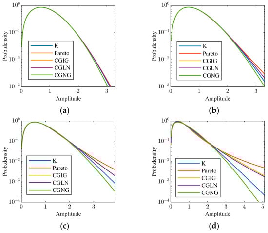
Figure 2.
Comparison of the tails of the five biparametric distributions when the parameters of the CGNG distributions take different values: (a) b = 1, λ = 0.1; (b) b = 1, λ = 0.5; (c) b = 1, λ = 1; (d) b = 1, λ = 2.
From the moments of the Nakagami distributions [20], the nth moment of the CGNG distributions is given by
The scale parameter b can be directly estimated by the second-order sample moment, and we can derive the following MoM (n = 1) estimator by taking n = 1:
where is the nth sample moment of the data and the estimate is obtained using the look-up table method. The [zlog(z)] estimator of the CGNG distributions can be given by a similar method as given in [31]. Let be sea clutter amplitude samples, and the estimates and are derived by
where Ψ(∙) is the Digamma function and the estimate is obtained using the look-up table method. As a new type of amplitude distribution, the two estimators above are new but straightforward. The two estimators behave well for clean clutter data. However, when radar echoes contain a fraction of outliers, their performance degrades severely. In addition, due to the absence of analytical expressions, the maximum likelihood (ML) estimator of the CGNG distributions is difficult to obtain, like in the CGLN distributions and the K-distributions [32,46].
One approach to obtain outlier-robust estimates is to use the biparametric CDF to fit the truncated empirical CDF (ECDF) of the data [47]. For an amplitude sample set probably containing a fraction of outliers, the samples are first sorted into in ascending order and the truncated data are obtained with the truncation ratio 0 < β < 1. The estimates and used to fit the truncated ECDF are given by
This numerical algorithm depends on initial points and is time-consuming. Therefore, it cannot be applied in practice and is often used as the benchmark to assess other outlier-robust estimators [32].
3. Outlier-Robust Tri-Percentile Estimators of CGNG Distributions
Due to the fact that the sample percentiles are robust to outliers, the outlier-robust bi-percentile estimators or tri-percentile estimators are proposed in succession for the four types of classic biparametric distributions [32,34,36,38]. In this section, we deal with the outlier-robust tri-percentile estimators of the CGNG distributions and the optimization of their parameter setup.
3.1. Outlier-Robust Tri-Percentile Estimators
For a positive number , the α-percentile of the parametric CDF is given by
where α is the percentile position and F−1(∙) is the inverse function of F(∙). In terms of the definition of moments and truncated moments [35], the percentile can be expressed as the zero-order truncated moment in form by
or the order statistics [48]. Zero-order truncated moments and order statistics are robust to a fraction of large amplitude outliers, which is the basis for the robustness of tri-percentile estimators to outliers. Like in [32,33,34,36,38], we attempt to build the relationship between the inverse shape parameter λ and the ratio of the two percentiles. In the context of the scale parameter b, given two percentile positions 0 < α < β < 1, the percentiles of and the percentiles of the scale-normalized distributions satisfy
Hence, the ratio is free of b and is uniquely determined by the two percentile positions (α, β) and the inverse shape parameter λ. However, this relationship is described by an implicit function. In terms of the CDF in (3), the implicit function is given by the following equation:
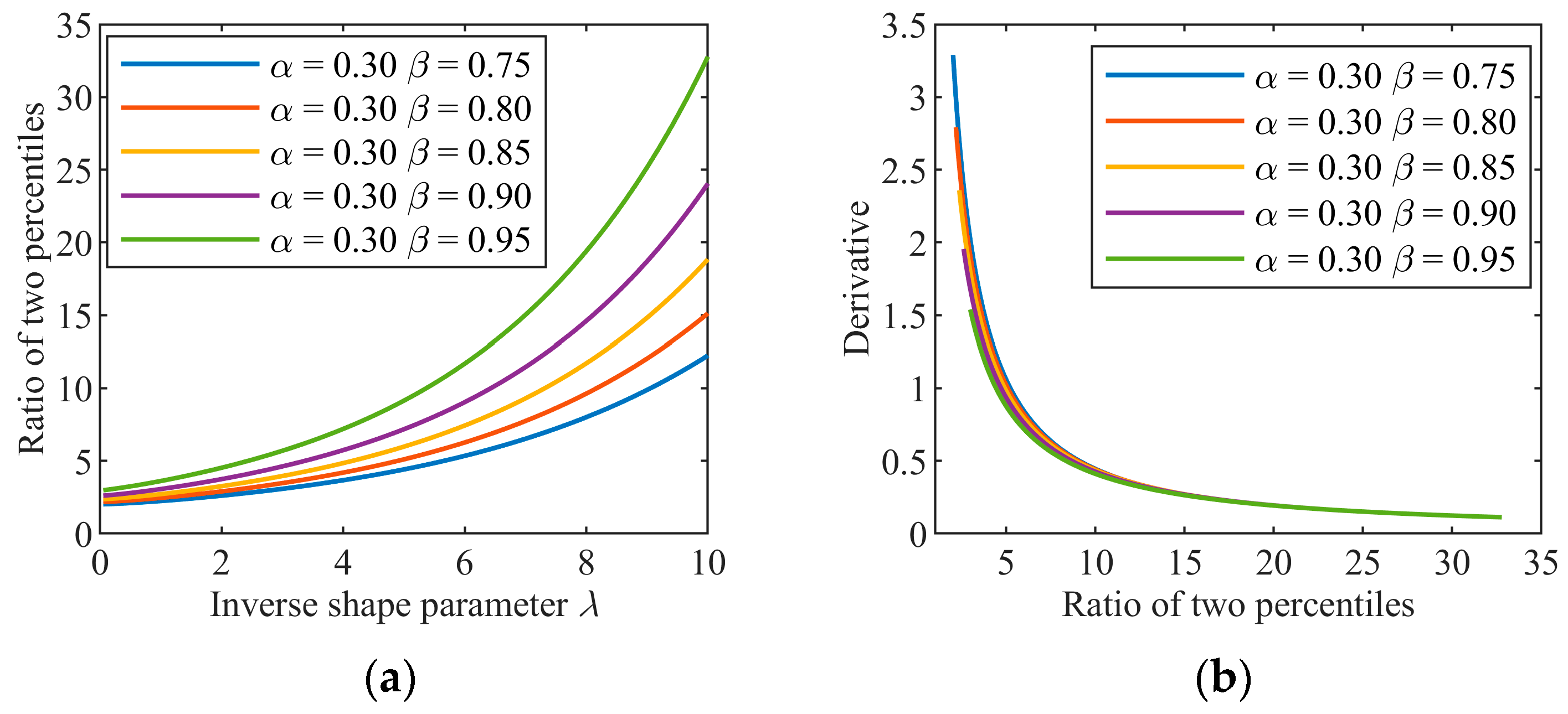
Obviously, for the given α, β, and λ, the ratio can be uniquely determined via computation. For the estimation of λ, the key is whether λ can be uniquely determined by the ratio of the two percentiles when their positions are given. In other words, whether the ratio is a monotonic function of λ determines whether λ can be successfully estimated. However, it is impossible to prove this conclusion due to the improper integrations with parameters in (12). In order for the completeness in theory to not impede parameter estimation in real applications, we use numerical computation to show that the ratio is the monotonic function of λ for a given (α, β). Figure 3a plots the curves of the ratio as λ changes from 0.05 to 10, where we take α = 0.30 and β = 0.75, 0.80, 0.85, 0.90, 0.95 as examples. The ratio monotonically increases with the inverse shape parameter λ. Hence, its inverse function does exist and can be expressed in form as follows:
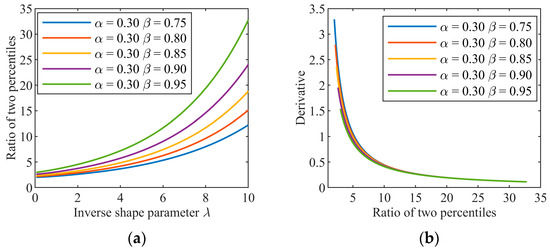
Figure 3.
(a) The ratio as a function of λ. (b) Derivative of the inverse function.
This function exists, but there is no closed-form solution. For a given (α, β), we can quickly obtain the value of λ using the look-up table method after a table is built via numerical computation. Figure 3b plots the graphs of the derivatives of the functions in (13) when α and β take values in term of Figure 3a. The derivatives take values at the interval [0.1, 3.5] when λ is in [0.05, 10] and are insensitive to the positions of α and β. Thus, λ markedly changes with the ratio but is not too sensitive to the ratio, which is helpful for robust estimation.
In the case that the inverse shape parameter λ is known in (13) and the position of the third percentile is given, we can obtain the scale parameter b. In terms of (3), the scale parameter is the solution of the following equation:
Naturally, there is no closed-form solution to the function in (14), and b is uniquely determined by λ and . In terms of (11), we can express the scale parameter b as a function of the third percentile in form by
The inverse function in the denominator must be obtained by the look-up table method after a table is built via numerical computation.
For the amplitude samples and the sorted samples , the three sample percentiles are estimated by
where [x] denotes the nearest integer to x. The estimates and of the two parameters are obtained by
This is referred to as the tri-percentile estimator of the CGNG distributions with a setup (α, β, γ). Obviously, the setup (α, β, γ) is important, as it affects the estimation performance.
3.2. Properties and Setup Optimization
The properties of sample percentiles determine the properties of the tri-percentile estimators. In fact, a sample percentile asymptotically follows the normal distribution when the sample size N tends to infinity [40], i.e.,
where represents the normal distribution with mean μ and variance . In terms of (18), the sample percentiles converge to the corresponding percentiles in probability when . In the tri-percentile estimators, the estimates of the scale and inverse shape parameters are both continuous functions of the three sample percentiles. Therefore, the estimates of the two parameters by the tri-percentile estimators both converge to their true values in probability when . Its proof is easy and can refer to the proof of the CGLN distributions [32].
Due to the fact that the two parameters vary on the half infinite line, the relative root mean squared error (RRMSE) is used to evaluate the estimation performance, which is defined by
In terms of the flow of the tri-percentile estimators, the first two percentile positions (α, β) are optimized to minimize the RRMSE(λ). In terms of (17), the estimate is obtained by the two sample percentiles or order statistics [48]. From the joint distribution of the two order statistics, we prove the following important property.
Property 1.
The RRMSEs of the inverse shape and scale parameters are free of the scale parameter.
The proof is given in Appendix A.
According to this property, we can let b = 1 when calculating the RRMSE of λ when the positions (α, β) and the sample size N take different values. Like in (20) [32,33,34,35,36,38], the selection of β is a compromise between robustness to outliers and estimation accuracy. The closer β is to one, the higher the estimation accuracy but the worse the robustness to outliers. It must be smaller than one minus the maximum possible percentage of outliers in the data, and thus β is often specified in advance in terms of the analysis of sea clutter environments. Moreover, for maritime radars, after outliers are excluded by simple detection, the percentage of outliers in the data is less than 5%. The value of β is recommended to be in the interval [0.8, 0.9] for real sea clutter environments. After β is determined, the optimal α is selected using the following optimization:
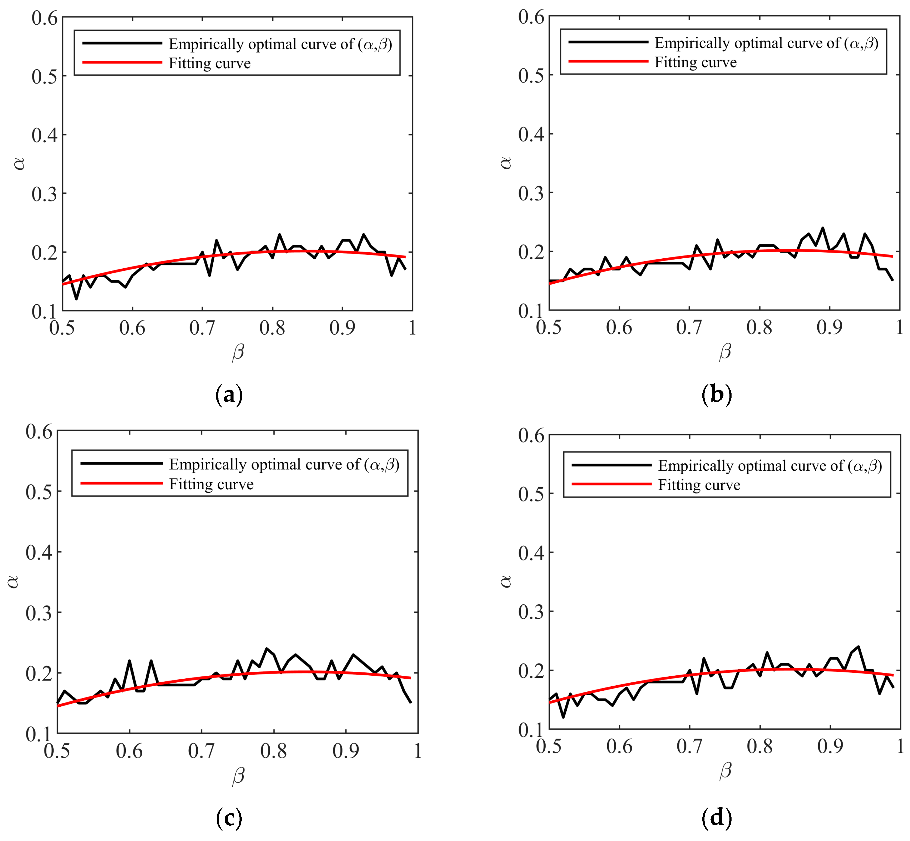
where is the prior distribution of λ. It is assumed to obey a uniform distribution of an interval when no prior information is available. The value of the two-variable function is calculated by a massive number of Monte-Carlo trials for a given sample size. From the equivalent line graph of the function, we find the optimal setup (α, β). The optimization (20) can be interpreted as minimizing the RRMSE(λ) subject to the outlier-robustness by limitation of the upper bound of β. Its dual problem becomes finding the minimal β subject to the upper bound of the RRMSE(λ). In this way, in terms of the dual problem, the optimal setup consists of the points on all the equivalent lines where β is minimal. In order to find the optimal setup curve, we calculate the RRMSE function for N = 103, 3 × 10³, 5 × 10³, and 104 when α varies from 0.1 to 0.6, β varies from 0.5 to 0.99, and the inverse shape parameter λ randomly takes a value in a uniform distribution of the interval [0.05, 10] in each trial. As shown in Figure 4, the black curves consist of the optimal setups at each sample size. We can find that the four black curves in Figure 4a–d are almost identical, and this phenomenon also appears for the other three types of distributions [32,36,38], though we fail to prove it. As shown in Figure 4, we use the red smooth curves to fit the four black curves well. The expression of the red smooth curve is given by
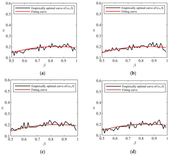
Figure 4.
Empirically optimal curve of (α, β) with different values of sample size N: (a) N = 1000; (b) N = 3000; (c) N = 5000; (d) N = 10,000.
Therefore, in the tri-percentile estimators, β is first selected based on the desired outlier-robustness and clutter environment, and then the optimal α is selected using the empirical function (21).
Once the estimate of the inverse shape parameter is obtained, we can estimate the scale parameter using the third sample percentile, whose position γ is optimized based on the asymptotic formula in (18). The coefficient of variation of the third sample percentile is the function of γ and λ. Its expression is given by
Obviously, the optimal γ depends on λ, and the optimal γ is given by
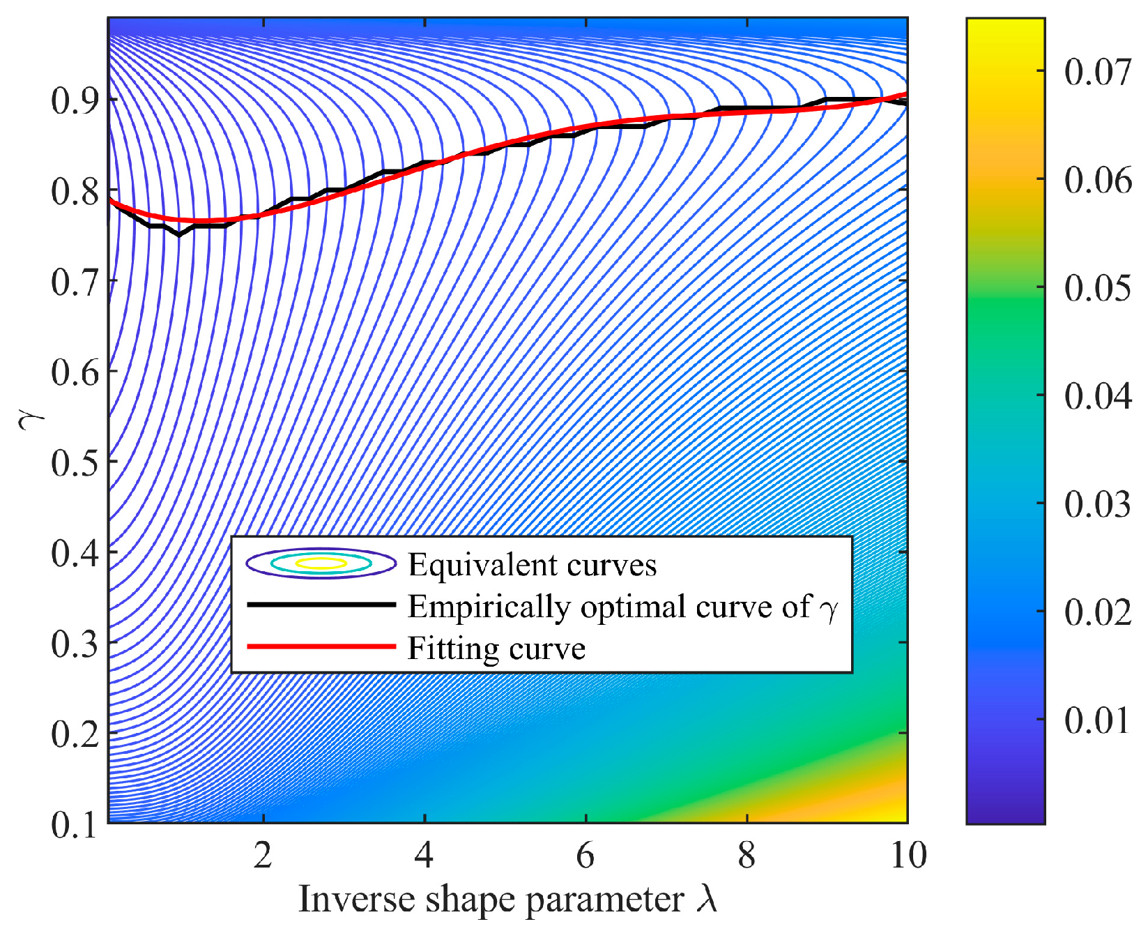
We calculate the value of function Ψ(λ, γ) and plot the corresponding equivalent curves as shown in Figure 5. The black curve is the optimal γ curve, which consists of the tangential points of the equivalent curves and the vertical lines. It is fitted by a smooth curve with the expression
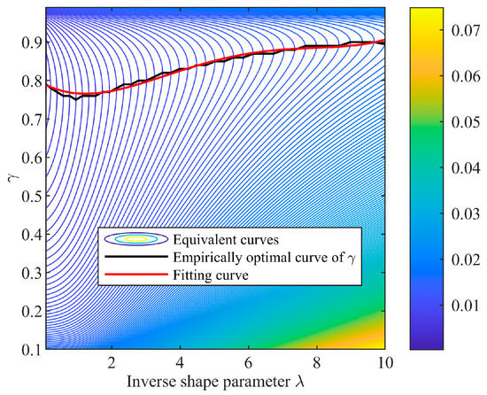
Figure 5.
Empirically optimal curve of γ.
In this way, the tri-percentile estimators with the optimal percentile position are constructed. β is first determined by the desired outlier-robustness and α is determined by β. The estimate is obtained by the two sample percentiles. At last, γ is determined by and the estimate is obtained by the third sample percentile. In addition, it is worth noting that γ must be taken as the smaller of the optimal values in (24) and β so as to assure robustness to outliers.
4. CGNG Model Suitability and Estimation Performance Comparison
In this section, we first verify the suitability of the CGNG distributions with an airborne Ku-band high-resolution sea clutter database. The K-distributions, CGIG distributions, CGLN distributions, generalized Pareto distributions, and the proposed CGNG distributions are used to fit sea clutter data at medium/high grazing angles. Next, the MoM (n = 1) estimator, the [zlog(z)] estimator, and the tri-percentile estimator (β = 0.85) are examined using simulated and measured data.
4.1. Suitability of CGNG Distributions
Besides the proposed CGNG distributions, there are at least four types of biparametric distributions for sea clutter modelling, the K-distributions [13], CGIG distributions [15], CGLN distributions [32], and generalized Pareto distributions [14]. Sea clutter data at different conditions need to be modeled by different types of distributions. Selecting the distribution type is the primary step in sea clutter modelling. Similar to the optimal distribution type selection of the X-band island-based dual-polarized high-resolution sea clutter data at low grazing angles [21], the optimal distribution type means that its fitted PDF or CDF is the closest to the empirical PDF (EPDF) or ECDF of the data. The geometric average of the KSD and the Kullback–Leibler divergence (KLD) [49] is used to measure the goodness-of-the-fit of the type. The two parameter estimates of the fitted PDF and CDF are obtained by the outlier-robust estimators in (8) where the truncated ratio β = 0.9 is used to alleviate the impact of a fraction of possible outliers existing in the data. The KSD and KLD are computed by
where and are the EPDF and ECDF of the data and are the estimated inverse shape and scale parameters determined by the estimators in (8). In fact, for the five types of distributions, as the inverse shape parameter tends to zero, the distributions converge to the Rayleigh distributions (corresponding to complex Gaussian clutter). Hence, in some cases, the five types of distributions have comparable goodness-of-the-fit, and every type of distribution is suitable for the data. In order to precisely assess the best type, the maximal selection benefit (MSB) of the best type on the data is defined by the ratio of the measure of the poorest type to that of the best type:
When the five types have comparable measures, the benefit of the optimal type is the smallest and close to one. The average value of the MSBs on the dataset where the type “A” is the best reflects the average benefit of the type on the dataset.
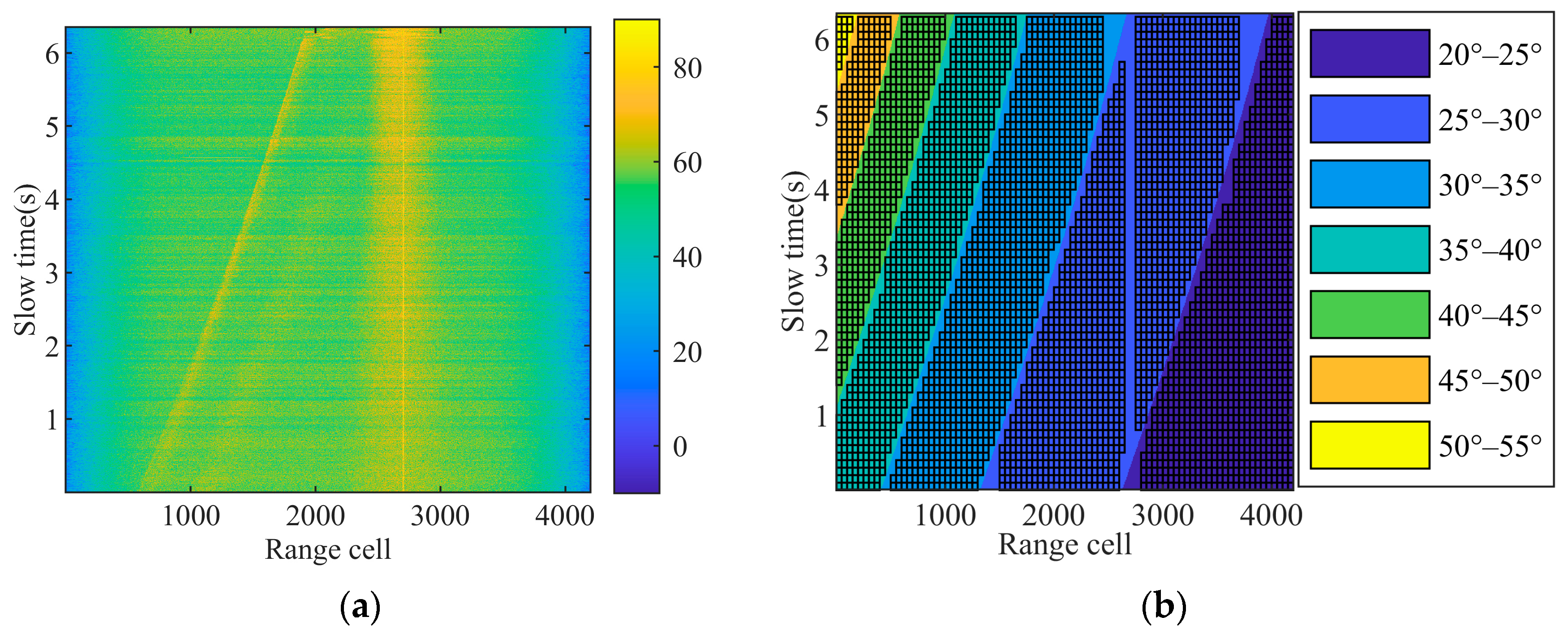
In order to examine the suitability of the CGNG distributions, the type selection from the five types of distributions are operated on one set of airborne high-resolution HH-polarized sea clutter data. The schematic diagram of the data collection is shown in Figure 6. The radar center frequency is 16.5 GHz, the pulse repetition frequency (PFR) is 10 KHz, the range resolution is 1.25 m, the azimuth beamwidth is 6 degrees, the grazing angle ranges from 20° to 55°, the height of the platform is 4500 m, and the aircraft flies steadily at about 100 m per second. During the measurement, the beam pointing of the antenna remains invariant. Figure 7a plots the power map of airborne Ku-band data in 4200 range cells and 6 s in decibels. As shown in Figure 7b, the data are divided into seven regions in terms of the grazing angles from 20° to 55° in an interval of 5°. Fifty successive range cells in each region consist of a clutter map cell (CMC) [50,51] and it is assumed that the sea clutter data in each CMC follows an amplitude distribution. For each CMC, the optimal type of distribution is selected in terms of the geometric average of the KSD and KLD in (25), where the parameters under each type are estimated by fitting the truncated ECDF in (8).
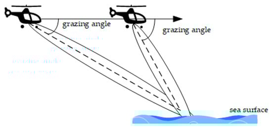
Figure 6.
Schematic diagram of medium/high grazing angle data collection.
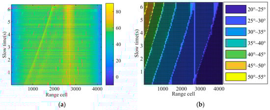
Figure 7.
(a) Power map of airborne Ku-band data (dB). (b) Region division in terms of the grazing angle and clutter map cell segmentation in each region where one net denotes a clutter map cell.
The numbers of CMCs in the seven regions and the percentages of each type considered to be the best are listed in Table 2. It can be seen that, in the seven regions, the percentages of the CGNG distributions considered to be the optimal type are largest, followed by the generalized Pareto distributions, K-distributions, the CGIG distributions, and the CGLN distributions. Therefore, the CGNG distributions are more suitable for Ku-band high-resolution sea clutter modelling and are at least competitive candidates. In addition, the percentages of the Rayleigh distributions considered to be the optimal type are below 1.1% in the seven regions. This shows that the Ku-band high-resolution sea clutter data at medium/high grazing angles deviate from Gaussian clutter. Furthermore, in order to evaluate the benefits of the optimal type selection of distributions, the average MSBs of every type on CMCs where it is the optimal type are listed in Table 3. It can be seen that, in four regions out of the seven regions, the CGNG distributions achieve the largest average MSB. Besides the largest percentages, the largest average MSBs over half of the regions show that the CGNG distributions are more suitable for modeling high-resolution sea clutter at medium/high grazing angles. Naturally, this conclusion from finite measured data still needs to be validated further by more measured data. At the least, from the results of these measured data, we can conclude that the CGNG distributions are one of the optimal distribution models for modeling high-resolution sea clutter at medium/high grazing angles.
Table 2.
Percentages of the five types of optimal distributions in the seven regions.
Table 3.
Average MSBs of every type of distribution in the seven regions.
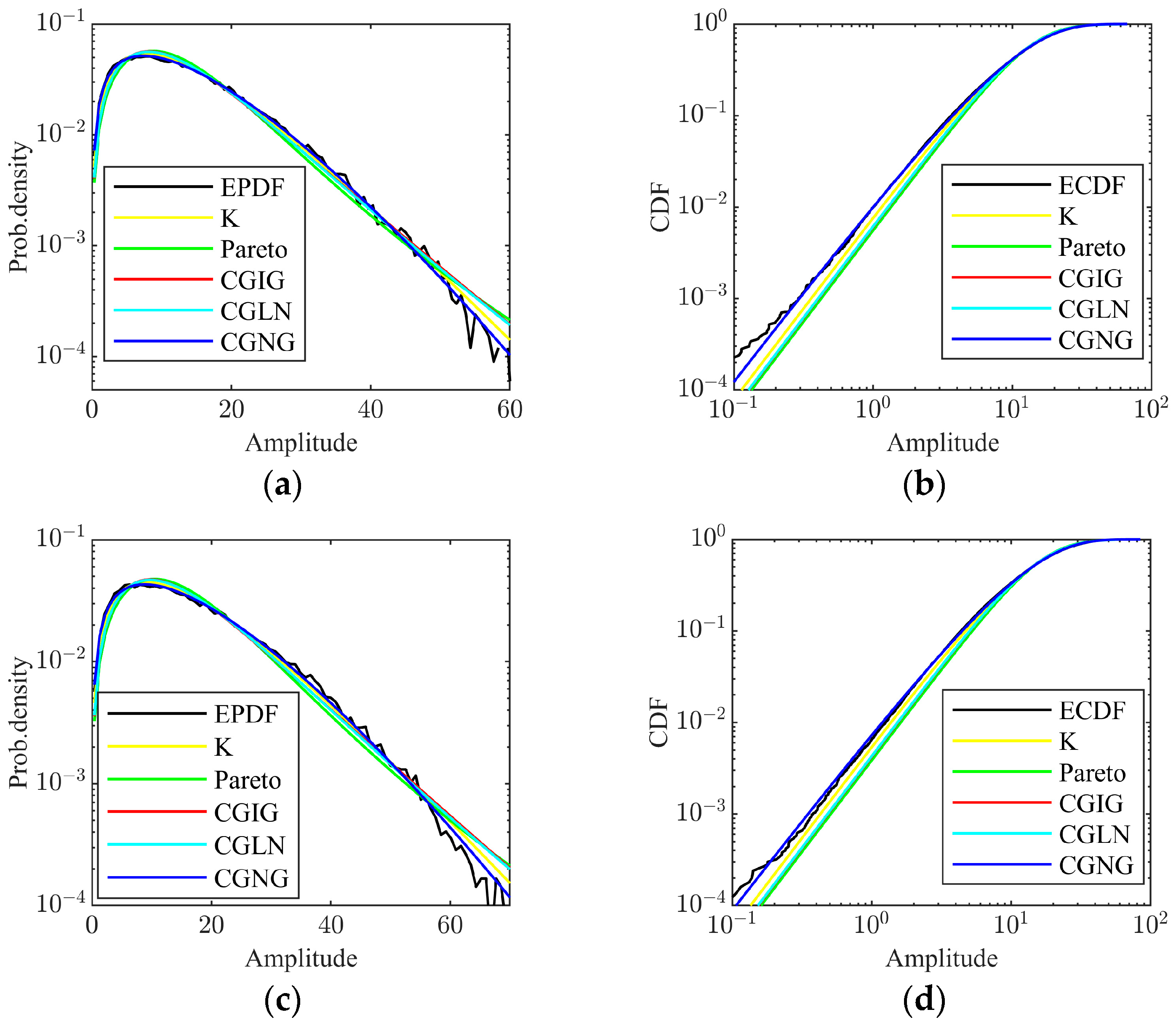
Moreover, in order to visually show the effect of the CGNG distributions, we select two CMCs, and plot the PDFs and CDFs of all the five fitted biparametric distributions and the EPDF and the ECDF of the data in Figure 8. It can be found that the CGNG distributions provide the best goodness-of-the-fit, especially on the tail parts of the EPDF. Moreover, the mean square error (MSE), KSD, and KLD between the fitted distributions and the empirical ones are listed in Table 4. It can be found that the CGNG distributions achieve the minimal MSE, KSD, and KLD at the two CMCs.
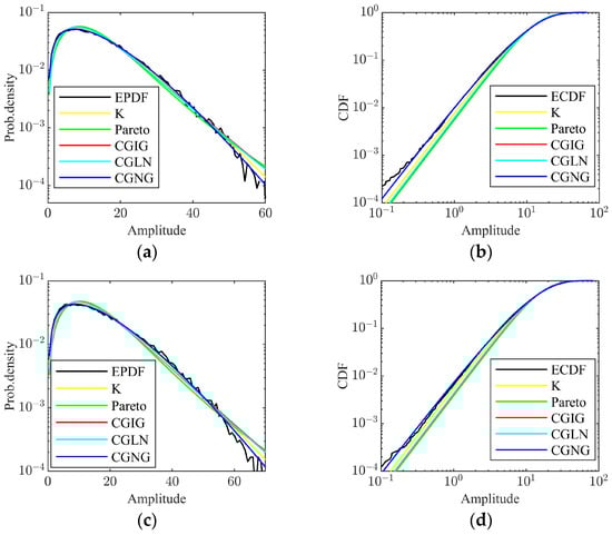
Figure 8.
Comparison of the performance of the five distributions in the two cases: (a) PDFs comparison in the case 1; (b) CDFs comparison in the case 1; (c) PDFs comparison in the case 2; (d) CDFs comparison in the case 2.
Table 4.
Results of the comparison of the five distributions in the two cases.
4.2. Performance Comparison of Tri-Percentile Estimators
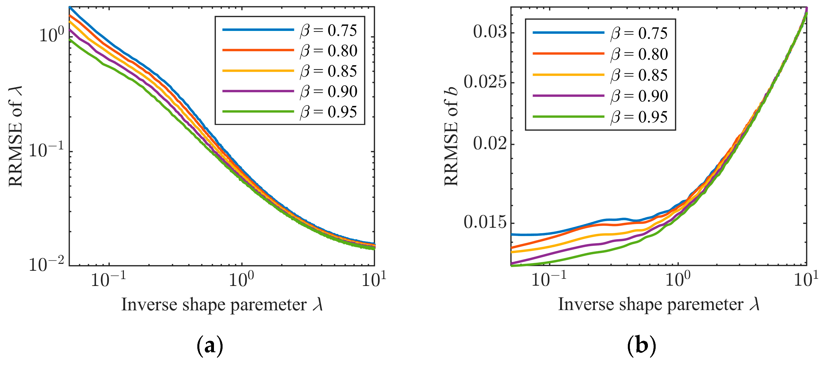
In this subsection, simulated data are first used to examine some properties of the proposed tri-percentile estimators with optimal percentile position setup. In the first experiment, β = 0.75, 0.80, 0.85, 0.90, 0.95 and the sample size is N = 104. We generate a set of simulated sea clutter sequences without outliers, and the RRMSEs of the inverse shape parameter λ and scale parameter b are plotted in Figure 9 as λ ranges from 0.05 to 10. In this case, as β is close to one, the RRMSEs become smaller, meaning that the estimator with a large β is a better choice for clean sea clutter data.
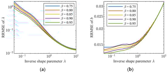
Figure 9.
RRMSEs of the estimated parameters with different values of β in the absence of outliers: (a) RRMSE of λ; (b) RRMSE of b.
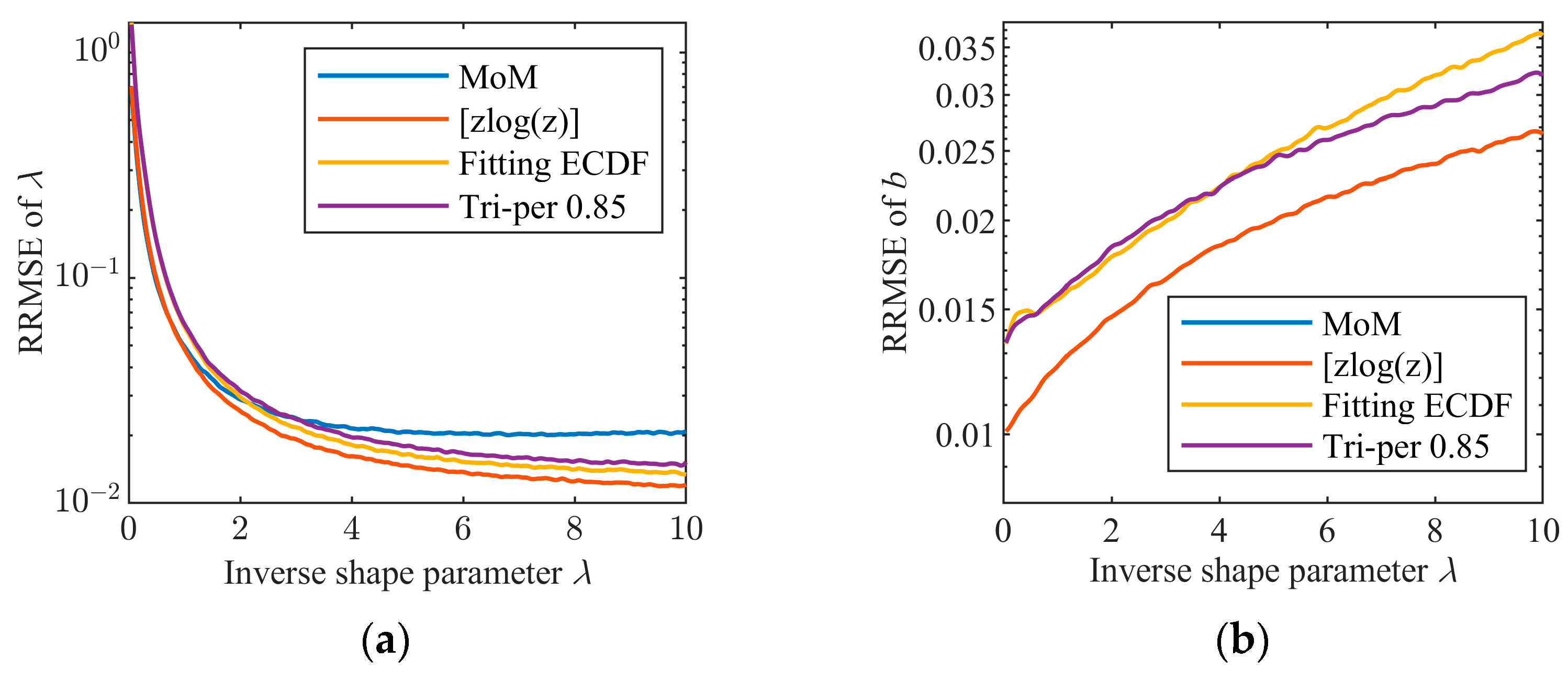
In the second experiment, the four estimators, including the MoM (n = 1) estimator, the [zlog(z)] estimator, the estimator fitting the truncated ECDF with the truncation ratio of 0.85, and the tri-percentile estimator (β = 0.85), are contrasted when the inverse shape parameter λ ranges from 0.05 to 10 and N = 104 in the absence of outliers. As shown in Figure 10, we plot the curves of the RRMSEs of the four estimators. In the estimation of λ, the four estimators have comparable performance, and the [zlog(z)] estimator and the estimator by fitting the truncated ECDF are slightly better than the other two estimators. In the estimation of b, the MoM (n = 1) estimator and [zlog(z)] estimator are obviously better than the other two estimators, owing to the fact that the first two directly estimate the scale parameter using the second-order sample moment while, for the latter two, one jointly estimates the two parameters and the other estimates the scale parameter with the help of the estimated inverse shape parameter. Overall, in the absence of outliers, all the four estimators can obtain acceptable estimation performance.
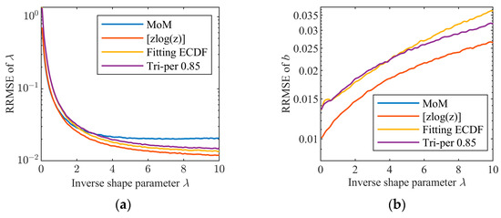
Figure 10.
RRMSE comparison of the four estimators of the CGNG distributions in the absence of outliers: (a) RRMSE of λ; (b) RRMSE of b.
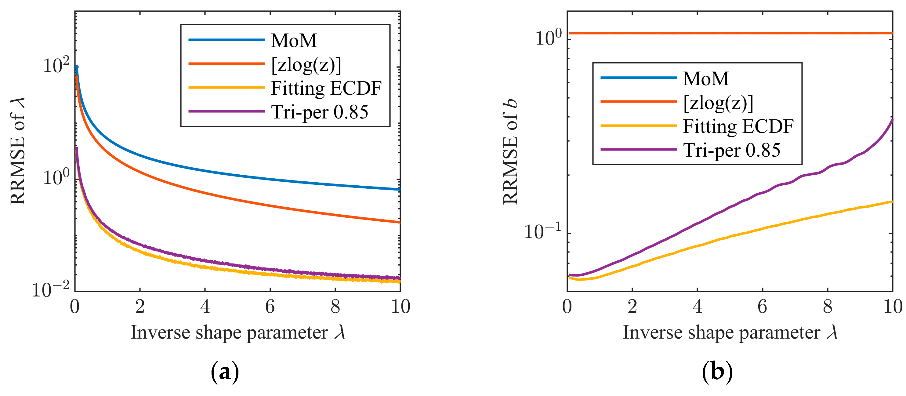
In the third experiment, the case with outliers is considered. The inverse shape parameter λ changes from 0.05 to 10, the scale parameter b = 1, and the sample size N = 104. Two percent of outliers whose intensities follow the uniform distribution in the interval [10b, 100b] are added to the simulated data. In this case, we plot the curves of the RRMSEs of the four estimators as shown in Figure 11. It can be seen that the outlier-robust tri-percentile estimator (β = 0.85) and the estimator fitting the truncated ECDF of data with the truncation ratio of 0.85 keep comparable performance with Figure 11 in the absence of outliers. However, the performance of the outlier-sensitive MoM (n = 1) estimator and [zlog(z)] estimator degrades sharply in comparison with the case without outliers in Figure 10. Therefore, in real clutter environments, outlier-robust estimators must be adopted.

Figure 11.
RRMSE comparison of the four estimators of the CGNG distributions in the presence of outliers: (a) RRMSE of λ; (b) RRMSE of b.
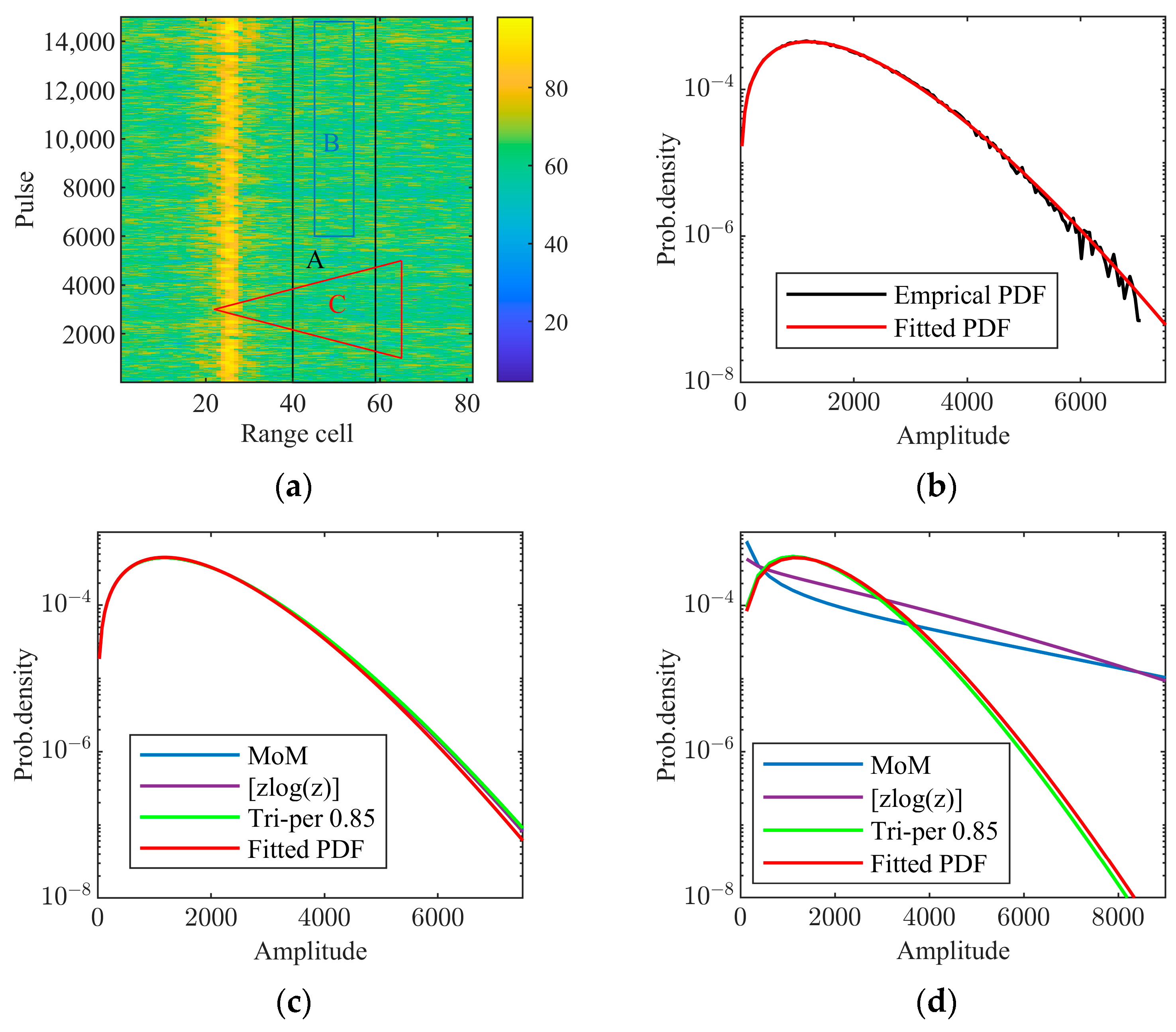
In the fourth experiment, Ku-band high-resolution airborne sea clutter data with a test target are used. The data consist of radar echoes of 15,000 successive pulses and 81 range cells at HH polarization, and the grazing angle is about 27°. A corner reflector located at the 25th range cell is used as the test target, and the radar echoes at the 24th and 26th range cells are affected by the corner reflector. In the parameter estimation of the CGNG distributions, the radar echoes at the 24–26th range cells are outliers. The power map of the data in decibels is plotted in Figure 12a. The pure clutter region A contains 3 × 10⁵ samples. In the CGM, the scale and inverse shape parameters are both in the expression of the texture distribution. Generally, for shore-based radars, the texture coherent length is over one hundred milliseconds [32]. For high-speed airborne radars, the texture coherent length becomes much shorter due to the relative movement between the radar and swells and large-scale wind waves on the sea surface. Using the JB test method in [16], the estimated texture coherent length of the measured data is about 3 milliseconds. As a result, 30 samples are at most equivalent to one independent and identically distributed (IID) sample in parameter estimation when the PFR is 10 KHz. In this way, 3 × 10⁵ samples in region A are at most equivalent to 104 IID samples, which is one case of a large sample size. The empirical amplitude PDF (APDF) in the region A and fitted APDF using the parameter estimates from the tri-percentile estimator (β = 0.85) are plotted in Figure 12b. The two highly accordant APDFs indicate the suitability of the CGNG distributions and the accuracy of the tri-percentile estimator (β = 0.85). Practical applications often encounter cases of moderate sample size. The rectangular region B in Figure 12a contains 88,000 pure clutter samples, corresponding to at most 2930 IID samples for parameter estimation, a case of a moderate sample size. Under the circumstances, the MoM (n = 1) estimator, the [zlog(z)] estimator, and the tri-percentile estimator (β = 0.85) are operated on the data to estimate the parameters. The APDF of the region A and the fitted APDFs using the parameter estimates from the three estimators are plotted in Figure 12c. The four curves are almost overlapped. Hence, in the absence of outliers in data, the three estimators can work well. To examine the cases with outliers, the triangular region C contains 88,000 samples including about 2% outliers from the corner reflector. Similarly, the three estimators are operated on the data for estimating the parameters of the CGNG distributions. The APDF of the region A and the three fitted APDFs by the parameter estimates from the three estimators are plotted in Figure 12d. We can find that the fitted APDF using the tri-percentile estimator (β = 0.85) can still approximate to the APDF of the region A while the fitted APDFs using the other two estimators deviate severely from the APDF of the region A and exhibit much heavier tails of amplitude distributions. Thus, the outlier-robust tri-percentile estimators of the CGNG distributions are rather important for practical applications of CGNG distributions in maritime radars.
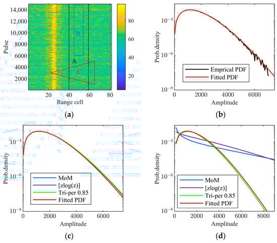
Figure 12.
Performance comparison of the tri-percentile estimator (β = 0.85), the MoM (n = 1) estimator, and [zlog(z)] estimator on the measured data: (a) power map of the measured data (dB); (b) fitting result in region A; (c) fitting result in region B; (d) fitting result in region C.
5. Conclusions
This paper introduces a compound-Gaussian model with Nakagami-distributed textures to model Ku-band airborne high-resolution sea clutter data at medium/high grazing angles. From this model, a new type of biparametric amplitude distributions, CGNG distributions for short, are derived to enrich the family of amplitude distributions of sea clutter, including the K-distributions, generalized Pareto distributions, CGIG distributions, and CGLN distributions. From the analysis of the measured data, it is found that the CGNG distributions are more suitable for modeling airborne Ku-band high-resolution sea clutter data at medium/high grazing angles. In addition, the outlier-robust tri-percentile estimators are proposed to robustly estimate the parameters of the CGNG distributions in the presence of outliers in data. The simulated data and measured data are used to examine the effectiveness of the tri-percentile estimators.
Author Contributions
Conceptualization, P.S. and G.Y.; methodology, G.Y. and X.Z.; software, P.Z.; validation and formal analysis, G.Y. and P.Z.; writing—original draft preparation, G.Y.; writing—review and editing, P.S.; supervision, P.S.; project administration, P.S.; funding acquisition, P.S. All authors have read and agreed to the published version of the manuscript.
Funding
This research was funded by in part by the National Natural Science Foundation of China under grant no. 62071346 and in part by the stabilization support of National Key Laboratory of Radar Signal Processing under grant no. KGJ202202.
Data Availability Statement
The data used in this study are not publicly available due to confidentiality restrictions.
Conflicts of Interest
The authors declare no conflicts of interest.
Appendix A
The RRMSE of the inverse shape parameter is first analyzed. Take the values of the percentile positions 0 < α < β < 1 and k1 = Nα, k2 = Nβ as two integers. According to the PDF and CDF in (3) and the joint PDF of the two order statistics [48], we can derive the following expression for the sample percentiles and :
In terms of (A1), the PDF of is
Hence, the PDF of is independent of b. In terms of (17), the estimate is obtained from , so the RRMSE of the inverse shape parameter λ is independent of the scale parameter b.
In what follows, the RRMSE of scale parameter b is analyzed. According to (15) and (17), we can use the mathematical expectation of the following random variable to represent the RRMSE of b
Because the PDF of the random variable is independent of the scale parameter b and the random variable is independent of b, the RRMSE of the scale parameter is independent of the scale parameter itself. However, the RRMSE of the scale parameter depends on the inverse shape parameter. The proof is completed.
References
- Gao, Y.C.; Liao, G.S.; Zhu, S.Q. Adaptive signal detection in compound-Gaussian clutter with inverse Gaussian texture. In Proceedings of the 2013 14th International Radar Symposium, Dresden, Germany, 19–21 June 2013; pp. 935–940. [Google Scholar]
- Shui, P.L.; Liu, M.; Xu, S.W. Shape-parameter-dependent coherent radar target detection in K-distributed clutter. IEEE Trans. Aerosp. Electron. Syst. 2016, 52, 451–465. [Google Scholar] [CrossRef]
- Xue, J.; Xu, S.W.; Shui, P.L. Near-optimum coherent CFAR detection of radar targets in compound-Gaussian clutter with inverse Gaussian texture. Signal Process. 2020, 166, 107236. [Google Scholar] [CrossRef]
- Xue, J.; Li, H.G.; Pan, M.Y.; Liu, J. Adaptive persymmetric detection for radar targets in correlated CG-LN sea clutter. IEEE Trans. Geosci. Remote Sens. 2023, 61, 5108212. [Google Scholar] [CrossRef]
- Xue, J.; Liu, J.; Xu, S.W.; Pan, M.Y. Adaptive detection of radar targets in heavy-tailed sea clutter with lognormal texture. IEEE Trans. Geosci. Remote Sens. 2022, 60, 5108411. [Google Scholar] [CrossRef]
- Xue, J.; Ma, M.S.; Liu, J.; Pan, M.Y.; Xu, S.W.; Fang, J. Wald- and Rao-based detection for maritime radar targets in sea clutter with lognormal texture. IEEE Trans. Geosci. Remote Sens. 2022, 60, 5119709. [Google Scholar] [CrossRef]
- Cumming, I.G.; Wong, F.H. Digital processing of synthetic aperture radar data. Artech House 2005, 1, 108–110. [Google Scholar]
- Pirkani, A.; Daniel, L.; Kumar, D.; Hoare, E.; Harris, S.; Cherniakov, M.; Stove, A.; Gashinova, M. Doppler Beam Sharpening for MIMO and Real Aperture Radars at mm-wave and Sub-THz Maritime Sensing. In Proceedings of the 2023 24th International Radar Symposium, Berlin, Germany, 24–26 May 2023; pp. 1–10. [Google Scholar]
- Zhang, Y.C.; Luo, J.W.; Zhang, Y.W.; Huang, Y.L.; Cai, X.C.; Yang, J.Y.; Mao, D.Q.; Li, J.; Tuo, X.Y.; Zhang, Y. Resolution enhancement for large-scale real beam mapping based on adaptive low-rank approximation. IEEE Trans. Geosci. Remote Sens. 2022, 60, 5116921. [Google Scholar] [CrossRef]
- Zhang, Y.C.; Luo, J.W.; Li, J.; Mao, D.Q.; Zhang, Y.; Huang, Y.L.; Yang, J.Y. Fast Inverse-Scattering Reconstruction for Airborne High-Squint Radar Imagery Based on Doppler Centroid Compensation. IEEE Trans. Geosci. Remote Sens. 2022, 60, 5205517. [Google Scholar] [CrossRef]
- Mezache, A.; Soltani, F.; Sahed, M.; Chalabi, I. Model for non-rayleigh clutter amplitudes using compound inverse gaussian distribution: An experimental analysis. IEEE Trans. Aerosp. Electron. Syst. 2015, 51, 142–153. [Google Scholar] [CrossRef]
- Sangston, K.J.; Gini, F.; Greco, M.S. Coherent radar target detection in heavy-tailed compound-Gaussian clutter. IEEE Trans. Aerosp. Electron. Syst. 2012, 48, 64–77. [Google Scholar] [CrossRef]
- Ward, K.D.; Watts, S.; Tough, R.J. Sea Clutter: Scattering, the K Distribution and Radar Performance, 2nd ed.; IET: London, UK, 2013; pp. 59–100. [Google Scholar]
- Balleri, A.; Nehorai, A.; Wang, J. Maximum likelihood estimation for compound-gaussian clutter with inverse gamma texture. IEEE Trans. Aerosp. Electron. Syst. 2007, 43, 775–779. [Google Scholar] [CrossRef]
- Ollila, E.; Tyler, D.E.; Koivunen, V.; Poor, H.V. Compound-Gaussian clutter modeling with an inverse Gaussian texture Distribution. IEEE Signal Process. Lett. 2012, 19, 876–879. [Google Scholar] [CrossRef]
- Carretero-Moya, J.; Gismero-Menoyo, J.; Blanco-Del-Campo, Á.; Asensio-Lopez, A. Statistical analysis of a high-resolution sea-clutter database. IEEE Trans. Geosci. Remote Sens. 2010, 48, 2024–2037. [Google Scholar] [CrossRef]
- Chalabi, I. High-resolution sea clutter modelling using compound inverted exponentiated Rayleigh distribution. Remote Sens. Lett. 2023, 14, 433–441. [Google Scholar] [CrossRef]
- Xue, J.; Xu, S.W.; Liu, J.; Shui, P.L. Model for non-Gaussian sea clutter amplitudes using generalized inverse Gaussian texture. IEEE Geosci. Remote Sens. Lett. 2019, 16, 892–896. [Google Scholar] [CrossRef]
- Gini, F.; Greco, M.V.; Diani, M.; Verrazzani, L. Performance analysis of two adaptive radar detectors against non-Gaussian real sea clutter data. IEEE Trans. Aerosp. Electron. Syst. 2000, 36, 1429–1439. [Google Scholar]
- Yacoub, M.D.; Bautista, J.E.V.; Guerra De Rezende Guedes, L. On higher order statistics of the Nakagami-m distribution. IEEE Trans. Veh. Technol. 1999, 48, 790–794. [Google Scholar] [CrossRef]
- Xia, X.Y.; Shui, P.L.; Zhang, Y.S.; Li, X.; Xu, X.Y. An empirical model of shape parameter of sea clutter based on X-band island-based radar database. IEEE Geosci. Remote Sens. Lett. 2023, 20, 3503205. [Google Scholar] [CrossRef]
- Gini, F.; Greco, M. Covariance matrix estimation for CFAR detection in correlated heavy tailed clutter. Signal Process. 2002, 82, 1847–1859. [Google Scholar] [CrossRef]
- Jay, E.; Ovarlez, J.P.; Declercq, D.; Duvaut, P. BORD: Bayesian optimum radar detector. Signal Process. 2003, 83, 1151–1162. [Google Scholar] [CrossRef]
- Shui, P.L.; Liu, M. Subband adaptive GLRT-LTD for weak moving targets in sea clutter. IEEE Trans. Aerosp. Electron. Syst. 2016, 52, 423–437. [Google Scholar] [CrossRef]
- Zaimbashi, A.; Norouzi, Y. Automatic dual censoring cell-averaging CFAR detector in non-homogenous environments. Signal Process. 2008, 88, 2611–2621. [Google Scholar] [CrossRef]
- Chalabi, I.; Mezache, A. Estimating the K-distribution parameters based on fractional negative moments. In Proceedings of the 2015 IEEE 12th International Multi-Conference on Systems, Signals & Devices, Mahdia, Tunisia, 16–19 March 2015; pp. 1–5. [Google Scholar]
- Chalabi, I.; Mezache, A. Estimators of compound Gaussian clutter with log-normal texture. Remote Sens. Lett. 2019, 10, 709–716. [Google Scholar] [CrossRef]
- Iskander, D.R.; Zoubir, A.M. Estimation of the parameters of the K-distribution using higher order and fractional moments [radar clutter]. IEEE Trans. Aerosp. Electron. Syst. 1999, 35, 1453–1457. [Google Scholar] [CrossRef]
- Mezache, A.; Bentoumi, A.; Sahed, M. Parameter estimation for compound-Gaussian clutter with inverse Gaussian texture. IET Radar Sonar Navig. 2017, 11, 586–596. [Google Scholar] [CrossRef]
- Yu, H.; Shui, P.L.; Huang, Y.T. Low-order moment-based estimation of shape parameter of CGIG clutter model. Electron. Lett. 2016, 52, 1561–1563. [Google Scholar] [CrossRef]
- Blacknell, D.; Tough, R.J.A. Parameter estimation for the K-distribution based on [zlog(z)]. IEE Proc.-Radar Sonar Navig. 2001, 148, 309–312. [Google Scholar] [CrossRef]
- Feng, T.; Shui, P.L. Outlier-robust tri-percentile parameter estimation of compound-Gaussian clutter with lognormal distributed texture. Digit. Signal Process. 2022, 120, 103307. [Google Scholar] [CrossRef]
- Shui, P.L.; Shi, L.X.; Yu, H.; Huang, Y.T. Iterative maximum likelihood and outlier-robust bipercentile estimation of parameters of compound-Gaussian clutter with inverse Gaussian texture. IEEE Signal Process. Lett. 2016, 23, 1572–1576. [Google Scholar] [CrossRef]
- Shui, P.L.; Yu, H.; Shi, L.X.; Yang, C.J. Explicit bipercentile parameter estimation of compound-Gaussian clutter with inverse gamma distributed texture. IET Radar Sonar Navig. 2018, 12, 202–208. [Google Scholar] [CrossRef]
- Xu, S.W.; Wang, L.; Zhang, F.Q.; Shui, P.L. Outlier-robust parameters estimation for compound-Gaussian clutter using inverse gamma texture based on truncated moments. Remote Sens. Lett. 2019, 10, 274–282. [Google Scholar] [CrossRef]
- Yu, H.; Shui, P.L.; Lu, K. Outlier-robust tri-percentile parameter estimation of K-distributions. Signal Process. 2021, 181, 107906. [Google Scholar] [CrossRef]
- Tian, C.; Shui, P.L. Outlier-robust truncated maximum likelihood parameter estimation of compound-Gaussian clutter with inverse Gaussian texture. Remote Sens. 2022, 14, 4004. [Google Scholar] [CrossRef]
- Shui, P.L.; Tian, C.; Feng, T. Outlier-robust tri-percentile parameter estimation method of compound-Gaussian clutter with inverse Gaussian textures. J. Electron. Inf. Technol. 2023, 45, 542–549. [Google Scholar]
- Xue, J.; Sun, M.L.; Liu, J.; Xu, S.W.; Pan, M.Y. Shape parameter estimation of K-distributed sea clutter using neural network and multi-sample percentile in radar industry. IEEE Trans. Ind. Informat. 2023, 19, 7602–7612. [Google Scholar] [CrossRef]
- Miao, Y.; Chen, Y.X.; Xu, S.F. Asymptotic properties of the deviation between order statistics and p-quantile. Commun. Stat. Theory Methods 2010, 40, 8–14. [Google Scholar] [CrossRef]
- Carretero-Moya, J.; Maio, A.D.; Gismero-Menoyo, J.; Asensio-Lopez, A. Experimental performance analysis of distributed target coherent radar detectors. IEEE Trans. Aerosp. Electron. Syst. 2012, 48, 2216–2238. [Google Scholar] [CrossRef]
- Daniel, W.W. Applied Nonparametric Statistics, 2nd ed.; PWS-Kent Pub: Boston, USA, 1990; pp. 319–330. [Google Scholar]
- Romik, D. Stirling’s approximation for n!: The ultimate short proof? Am. Math. Mon. 2000, 107, 556–557. [Google Scholar] [CrossRef]
- Stephens, M. EDF statistics for goodness of fit and some comparisons. J. Am. Stat. Assoc. 1974, 69, 730–737. [Google Scholar] [CrossRef]
- Watts, S.; Rosenberg, L. A review of high grazing angle sea-clutter. In Proceedings of the 2013 International Conference on Radar, Adelaide, Australia, 9–12 September 2013; pp. 240–245. [Google Scholar]
- Roberts, W.J.J.; Furui, S. Maximum likelihood estimation of K-distribution parameters via the expectation-maximization algorithm. IEEE Trans. Signal Process. 2000, 48, 3303–3306. [Google Scholar]
- Mezache, A.; Sahed, M.; Laroussi, T.; Chikouche, D. Two novel methods for estimating the compound K-clutter parameters in presence of thermal noise. IET Radar Sonar Navig. 2011, 5, 934–942. [Google Scholar] [CrossRef]
- Balakrishnan, N.; Clifford Cohen, A. Order Statistics and Inference; Academic Press: New York, NY, USA, 1991; pp. 7–17. [Google Scholar]
- Weinberg, G.V.; Glenny, V.G. Optimal Rayleigh approximation of the K-distribution via the Kullback–Leibler divergence. IEEE Signal Process. Lett. 2016, 23, 1067–1070. [Google Scholar] [CrossRef]
- Conte, E.; Bisceglie, M.D.; Lops, M. Clutter-map CFAR detection for range-spread targets in non-Gaussian clutter. II. Performance assessment. IEEE Trans. Aerosp. Electron. Syst. 1997, 33, 444–455. [Google Scholar] [CrossRef]
- Conte, E.; Lops, M. Clutter-map CFAR detection for range-spread targets in non-Gaussian clutter. I. System design. IEEE Trans. Aerosp. Electron. Syst. 1997, 33, 432–443. [Google Scholar] [CrossRef]

Disclaimer/Publisher’s Note: The statements, opinions and data contained in all publications are solely those of the individual author(s) and contributor(s) and not of MDPI and/or the editor(s). MDPI and/or the editor(s) disclaim responsibility for any injury to people or property resulting from any ideas, methods, instructions or products referred to in the content. |
© 2024 by the authors. Licensee MDPI, Basel, Switzerland. This article is an open access article distributed under the terms and conditions of the Creative Commons Attribution (CC BY) license (https://creativecommons.org/licenses/by/4.0/).